ASYMMETRICAL MATING PREFERENCES
HÉLÈNE LEMAN
Abstract. More and more evidence shows that mating preference is a mechanism that can lead to a reproductive isolation event. In this paper, we consider a haploid population living on two patches linked by migration. Individuals are ecologically and demographically neutral on the space and differ only on a trait,a or A, determining both mating success
and migration rate. The special feature of this paper is to assume that the strength of the mating preference and the migration depend on the trait carried. Indeed patterns of mating preferences are generally asymmetrical between the subspecies of a population. We prove that mating preference alone can lead to a reproductive isolation and we explicit the time before reproductive isolation occurs. To reach this result we use an original method to study the limiting dynamical system, analyzing first the system without migration and adding migration with a perturbation method. Then using simulations, we study the time before reproductive isolation with respect to the strength of migration and the strength of both mating preferences, highlighting that large migration rates tend to favor the most permissive types.
Keywords: mating preference, asymmetrical preference, birth-death stochastic model, dy-namical system, long-time behaviour, perturbation method.
AMS subject classification: 92D40, 37N25, 60J27. 1. Introduction
Understanding the mechanisms of speciation and reproductive isolation is a major issue in evolutionary biology. There exist more and more evidences of links between sexual preferences and speciation [26, 5]. Historically, the role of ’magic’ or ’multiple effect’ traits, which combine adaptation to an ecological niche and mating preference, have been studied first. It has been shown that such traits can lead to speciation using direct experimental evidence [28] or theoretical works [25, 39]. The emerging issue is now to separate the role of sexual selection, and in particular of mating preference, from other mechanisms in a speciation event [16]. Panhuis et al [30] wrote that for example, the initial divergence in traits or preferences may be the result of natural selection in order to decrease hybridization and then be subject to sexual selection. Some studies have illustrated the promoting role of sexual preference alone, using numerical simulations [24, 29, 35], or theoretical results [32, 10]. However, those studies focus on a symmetrical sexual preference, assuming that any type of individuals express the same strengh in the sexual preference contrary to the experimental observations in general. Here, we generalise the model of Coron et al. [10] to take into account an asymmetry between the types.
This paper is motivated by the numerous examples of species that express an asymmetrical pattern of preference (See Panhuis et al. [30] for examples). Smadja et al. [37] describe such an example between two subspecies of the house mouse. The subspeciesMus musculus mus-culus is characterized by a stronger assortative preference than the subspeciesMus musculus domesticus [36]. A mechanism for subspecies recognition mediated by urinary signals occurs between those two taxa and seems to maintain a reproductive isolation. Another example comes fromDrosophila melanogaster populations that also show strong sexual isolation with an asymmetrical pattern. The Zimbabwe female lines have a nearly exclusive preference for
1
males from the same locality over the males from other regions or continents; the reciprocal mating is also reduced but to a lesser degree [40, 19]. In this paper, we will be interested in two main problematic: studying the influence of an asymmetric mating preference on the speciation mechanism and understanding the effects of migration on sexual preference selection.
As done by Coron et al [10], we consider a haploid population distributed on two demes linked by migration. Following the seminal papers [4, 12, 15], we use a stochastic individual-based model with competition and varying population size. We assume that individuals do not express any local adaptation such that their parameters do not depend on their location. However, individuals are characterized by a mating trait, encoded by a bi-allelic locus, and which has two consequences: individuals of the same type have a higher probability to mate and give an offspring, and the rate of migration of an individual increases with the proportion of individuals of the other trait in its deme. Besides, in order to generalize [10], we assume that the two locus can have asymmetrical effects : the strength of the mating preferences and of the migration depend on the locus of the individual.
First, in a classical large population limit, we connect our microscopic model to a limiting deterministic model. Then, we study both the stochastic individual-based model and the limiting deterministic model in order to derive our main result : we prove that there is reproductive isolation and we give the time needed before this event. Here, contrary to [10], the time is related to both mating preference parameters and both migration parameters coming from the two different loci. Besides, we conduct an extensive study on the influence of the migration and preference parameters on this time showing that large migration rates can facilitate the most permissive type to survive (i.e. the type with a reduced mating preference). The proof of the main result is based on a fine analysis of the deterministic limiting model. In particular, we are able to derive global results on the dynamical system such that we understand the behaviour of almost all the trajectories. To this aim, we develop an original method based on a perturbation theory of the migration parameters, which fully differs from the method used by Coron et al. [10]. The asset of our method is the possibility to adapt it easily to other dynamical systems.
The structure of the paper is the following one. In Section 2, we introduce the stochastic model and we motivate it from a biological perspective. Section 3 expounds the results of the paper. In particular, in Section 3.1, we state the main results on the deterministic limiting model and on the stochastic process. Section 3.2 presents the main result in the case without migration between the two patches. In Section 3.3, we examine the influence of the migration on the time before reproductive isolation. Finally, Section 4 is devoted to the proof of the key result of this paper using a perturbation theory. We let the proofs of the case without migration in Appendix A and the probabilistic parts of the proofs in Appendix B since they are generalisations of the proofs in Coron et al. [10].
2. Model
The population is divided between two patches. The individuals are haploid and charac-terized by a mono-allelic locus (a or A) and their position (1 or 2 depending on the patch they lay). The dynamics of the population follows a multi-type birth and death process with competition in continuous time. Let us denote the set {(α, i), α ∈ {a, A}, i ∈ {1,2}} by E. Hence, the dynamics follows a Markov jump process in the space NE, where the rates are described below.
by the vector of dimension 4 inNE:
NK(t) = (NA,K1(t), Na,K1(t), NA,K2(t), Na,K2(t))∈NE whereNK
α,i(t)denotes the number of individuals with genotypeα in the demeiat timet. In what follows, ifα denotes one of the allele, we use the notation α¯ to denote the other allele and if idenotes one of the deme,¯idenotes the other one.
We now explicit the birth, death and migration rates that give the dynamics of the popu-lation in the two demes.
At a rate B >0, a given individual with trait α ∈ {a, A} encounters uniformly at random another individual of its deme. Then it mates with this other individual and transmits its trait with probabilitybβα/B≤1if the other individual carries also the traitαand with prob-ability b/B≤1if the other individual carries the traitα¯. That is to say, after encountering, two individuals that carry the same trait α have a probability βα-times larger to mate and give birth to a viable offspring than two mating individuals with different traits. Hence, if we denote byn∈NE the current state of the population, the total birth rate of α-individuals in the patch iwrites
(2.1) bnα,i
βαnα,i+nα,i¯
nα,i+nα,i¯
.
Note that we use two parameters to model the sexual preference depending on the trait the individual carries : βa and βA. The limiting case where βA =βa was studied by Coron et al. [10]. In our paper, we will be interested in the case where βa6=βA although we will find again the result of the limiting case with our calculation. As presented in [10], Formula (2.1) models an assortative mating by phenotypic matching or recognition alleles [3, 21]. Note that, in our model, the preference modifies the rate of mating and not only the distribution of genotypes, unlike what is usually assumed in classical generational model [26, 23, 7, 34]. However, we can compare our model with the classical ones by computing the probabilities that an individual of traitαin the deme igives birth after encountering an individual of the same trait (resp. of the opposite trait) conditionally to the fact that this individual gives birth at time t, and we find
βαnα,i βαnα,i+nα,i¯
resp. nα,i¯ βαnα,i+nα,i¯
.
Note that those terms correspond to the ones presented in the supplementary material of Servedio [34], or Gavrilets and Boake [17] (case n = +∞). A extended discussion between those two types of model can be found in Section 2 of [10].
The death rate of a given individual is composed of a natural death rate and a competition death rate. All individuals compete for resources or space against all individuals in the same deme. The death rate of each individual due to competition is proportional to the size of the population in its deme. Finally, the total death rate of α-individuals in the patch iwrites
(2.2) d+ c
K (nα,i+nα,i¯ )
nα,i,
where d models the natural death and c models the competition for resources. Recall that K is a scaling parameter. Actually, it is related with the carrying capacities and it scales the amount of available resources. Hence asKis larger, the strength of competition between two individuals decreases.
individuals of the other trait in its deme and to a parameter pα which depends on the trait of the individual. Hence, the genotypes express different strength in the sexual preference and in the migration speed. The total migration rate of α-individuals from patch1 to patch
2 finally writes
Note that the migration rate does not depend on the state of the other deme.
In what follows, we assume the following statements on the parameters:
βA>1, βa>1, b > d >0, c >0, pA≥0, pa≥0.
3. Results
3.1. Time needed before reproductive isolation. In this section, we present the main result of the paper that gives the time needed for the process NK to reach reproductive isolation. This time is given with respect toK, the carrying capacity of the process.
To this aim, let us first give the average behaviour of the process using a convergence in large population limit. Precisely, Lemma 3.1 below ensures that the sequence of re-scaled processes
converges whenK goes to infinity to (3.1)
Lemma 3.1. Assume that the sequence (ZK(0))
K≥0 converges in probability to the
deter-ministic vector z0 ∈RE. Then, for any T ≥0,
t≥0 denotes the solution to (3.1) with
initial condition z0 ∈RE
This result can be deduced from a direct application of Theorem 2.1 p. 456 by Ethier and Kurtz [14] or from Lemma 1.1. of [10].
Using a direct computation, we can see that the four states
(3.3) (ζA,0,0, ζa), (ζA,0, ζA,0), (0, ζa, ζA,0), (0, ζa,0, ζa),
whereζα:= bβαc−d, forα∈ {A, a}, are four equilibria to the system (3.1). Then let us define the weighted sums
Σi := (βA−1)zA,i+ (βa−1)za,i, for i= 1,2,
Next Lemma ensures that we can restrict the study to the trajectories starting from the compact set
(3.4) S :=nz∈RE,Σi≥
(βA∧βa−1)(b−d)
4c for i= 1,2,
andΣ≤22b(βa∨βA)
(βA∨βa−1)−d
c
o ,
since any trajectory reaches it in finite time.
Lemma 3.2. Assume that
(3.5) pA(βA−1) +pa(βa−1)≤2(b−d)(βA∧βa−1).
S is an invariant set for the dynamical system (3.1) and any trajectory solution to (3.1) hits
S after a finite time.
The aim is thus to study the trajectories inside the compact setS.
Theorem 3.1. (1) Assume that pA= 0 if and only if pa= 0. There exists p0 >0 such
that for all pA ≤ p0 and pa ≤ p0, we can find four open subsets (Dα,α
′
pA,pa)α,α′∈A of S which are the basins of attraction in S of the four equilibria (3.3) under the sys-tem (3.1) and such that the adherence of∪α,α′∈ADα,α
′
pA,pa is equal to S. (2) In the case pA=pa= 0, the basins of attraction are exactly
D0α,α,0′ =
z∈RE,(βα−1)zα,1 >(βα¯−1)zα,¯1 and (βα′−1)zα′,2 >(βα¯′−1)zα¯′,2 ∩ S.
Theorem 3.1 is a key result to deduce the main result of our paper. It ensures that any trajectory starting from S, except from an empty interior set, reaches one of the steady states (3.3). The result can be compared with Theorem 2 of [10] which gives the same kind of results in the symmetrical case (βA=βaandpA=pa). In contrast with it, the equilibrium reached does not depend on the genotype which is initially in majority in each patch but the dynamics is more involved. In the case without migration, the equilibrium reached depends on a weighted difference between the initial number of individuals of each type, weighted by the strength of the preference. For pA, pa small, the basin of attraction Dα,α
′
pA,pa is actually a deformation ofD0α,α,0′. We will draw an example of such basin of attraction in Section 3.3. Hence, the asymmetrical sexual preferences make the long time behavior more involved than in the symmetrical case and the proof here uses complete different mathematical techniques since the dynamical system satisfied by the sums and the differences in each deme is not simple. We use here a perturbation method to deduce Theorem 3.1 : we study the system in the particular case where pA = pa = 0, and we make pA and pa grow up to deduce the result for some positive migration rates. Unfortunately, we are not able to give an explicit formulation for the setsDpα,α′ unlike in the symmetrical case.
We are now ready to state the main result of this section.
Theorem 3.2. Assume that Assumptions of Theorem 3.1 holds and thatpA≤p0andpa≤p0.
Let ε0 > 0 and assume also that ZK(0) converges in probability to a deterministic vector
z0 ∈ DpA,aA,pa such that (za,01, zA,0 2)6= (0,0). Let us set for any ε >0:
Then there exist C0 > 0 and m > 0, and a positive constant V depending on (m, ε0) such
Similar results hold for the three other equilibria of (3.3).
TK
BA,a,ε is the random time before all the a-individuals in the patch 1 and all the A -individuals in the patch 2 get extinct. Hence Theorem 3.2 gives the order of time needed before reaching this extinction: the time is proportional to the logarithm of the carrying capacity,log(K).
Secondly, the assumption on the initial condition(za,01, z0A,2)6= (0,0)is only needed to obtain the lower bound on the timeTK
BA,a,ε in (3.6). Otherwise, this time would be faster.
Finally, note that we find again the result for the symmetrical case (βA = βa) which was presented in Theorem 3 in [10]. Furthermore, in the asymmetrical case (βA6=βa), the time needed to reach the equilibrium depends on the equilibrium reached through the inverse of ω(α, α′). When the equilibrium reached is composed of A-individuals in a patch and a -individuals in the other one, the time depends also on the two migration rates pA and pa. We will study the influence of the migration rates on this extinction time in Section 3.3.
3.2. System without migration. The proofs of the theorems of the previous section call for full understanding of the dynamics of the system without migration. Hence before proceeding with the proofs, we present the study of the dynamical system when pA = pa = 0. Since the two patches evolve independently in this case, we only study the dynamics in the patch 1 and we drop the dependency with the patch in the notation, for the sake of simplicity. From (3.1), we derive that
The equilibria of the system write with the following quantities
χα:= (βα¯−1)χ, where χ:=
b(βa−1)(βA−1) + (b−d)(βA−1 +βa−1) c(βA−1 +βa−1)2
,
and where α¯ =A \α if α∈ A. Using a direct computation, we find that there exist exactly four fixed points of the dynamical system (3.8):
(0,0), (ζA,0), (0, ζa), and (χA, χa).
Let us describe the stability of the equilibria and the long time behavior of any solution to (3.8).
Lemma 3.3. • (ζA,0)and(0, ζa)are two stable equilibria,(0,0)is unstable and(χA, χa)
• The set
(3.9) DA
0 :=
(zA, za)∈R2,(βA−1)zA>(βa−1)za
is an invariant set under the dynamical system (3.8). Moreover, any solution which starts from the set DA
0 converges to (ζA,0) whent converges to +∞. • The set
Da
0 :={(zA, za)∈R2,(βa−1)za>(βA−1)zA},
is an invariant set under the dynamical system (3.8). Any solution which starts from the set Da
0 converges to (0, ζa) whent converges to +∞.
• Finally, {(zA, za) ∈ R,(βA−1)zA = (βa −1)za} is also an invariant set and any
solution which starts from this set converges to (χA, χa) when tgrows to +∞.
Using this Lemma, we deduce directly that the basin of attraction D0α,α,0′ are the ones
described by Theorem 3.1.
3.3. Influence of the parameters on the time before reproductive isolation. In this section, we come back to the initial model, with two demes. We use functional studies and simulations to explore the influence of the migration rates and the mating preference parame-ters on the process. The following simulations are computed with the following demographic parameters:
(3.10) βA= 2, βa= 1.5, b= 2, d= 1 and c= 0.1, unless stated otherwise. For these parameters,
ζA= 30 and ζa= 20.
Influence of the parameters on the macroscopic time: Firstly, we study how the constant of the macroscopic time before reproductive isolation is modified when the migration rates and the mating preference parameters vary. Assume that the process starts from a state where it reaches a neighborhoodBA,a,ε of equilibrium(ζA,0,0, ζa). We are thus interested in the variation of the constant1/ω(A, a). Direct functional studies ensure that this constant is a decreasing function with respect toβA or toβawhatever are the other parameters. Hence, stronger is the sexual preference, faster is the reproductive isolation.
Then, how does it evolve with respect topA and pa. It may be natural to consider that pA and pa can be rewritten using three positive parametersγA,γa and pas follows:
pA:=γAp and pa:=γap.
It is a way to consider that the two parameters of migration evolve at the same time. Once again, a direct functional study ensures that 1/ω(A, a) is a non-increasing function with respect to p. On Figure 1, we present how the value 1/ω(A, a) changes with respect to p when the parameters are defined by (3.10). Hence, increasing both migration rates at the same time accelerates the reproductive isolation. Since this trend is in line with the change of 1/ω(A, a) with respect to the mating preference parameters and in view of the migration terms we chose, our first conclusion is then : a large migration rate seems to strengthen the homogamy.
Figure 1. Graphs of the constants of the extinction time, 1/ω(A, a) (blue line), 1/ω(A, A) (red dashed line), 1/ω(a, a) (red dashed-dotted line), with respect top(left) and toβA(right). The demographic parameters are defined by (3.10),γA= 1,γa=βa−1 = 0.5and βA= 2 on the left andp= 2 on the right.
before reproductive isolation, which is more surprising. In particular, it ensures that a large migration rate does not only reflect a strong sexual preference but implies more involved behavior, which will be confirmed in what follows.
Basins of attraction : We now explore how the basin of attraction are modified when the migration rates increase. To simplify the study, we assume here thatp:=pA=pa.
Figure 2 presents the trajectories of some solutions to the dynamical system (3.1) in the two phase planes which represent the two patches. We plot the trajectories for the initial condition
zA,1(0) = 4, za,1(0) = 10, zA,2(0) = 8.5 and za,2(0) = 15,
and for three different values of p: 0,1and 5. It is important to notice that the equilibrium
0 2 4 6 8 10 12 14 16 18 20
0 5 10 15 20 25 30
Pat ch 1
0 2 4 6 8 10 12 14 16 18 20
0 5 10 15 20 25 30
Pat ch 2
Figure 2. Plots of the trajectories in the phase planes which represent the patch
1 (left) and the patch2 (right) fort∈[0,10]and for three values ofp: p= 0(red),
p= 1(blue), p= 5 (green). The initial condition is(4,10,8.5,15), represented by
the black dots. The dark line is the solution to(βA−1)zA−(βa−1)za = 0
converges to (0, ζa,0, ζa). Hence, a large migration ratepcan help the more permissive type a(βa< βA) to invade the two patches.
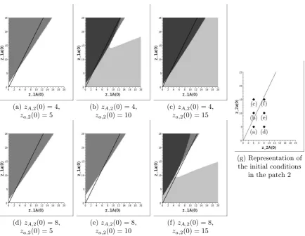
Secondly, we give an example of the basins of attraction Dp,pα,α′ for a large migration rate p. Figure 3 presents the projections of the four sets on six different planes for p = 5. In other words, each graph (a-f) represents the equilibrium reached with respect to the initial condition in the deme1 for a couple of initial conditions in the deme2 which is represented on the graph (g). In order to compare the results for p= 5 and for p = 0, we plot the line solution to (βA−1)zA,1−(βa−1)za,1 = 0 on the planes. Indeed, according to Lemma 3.3,
without migration any trajectory with initial conditions in the patch 1 above (resp. below) this line converges to a patch filled with a-individuals (resp. A-individuals). Generally, we
(a)zA,2(0) = 4,
za,2(0) = 5
(b)zA,2(0) = 4,
za,2(0) = 10
(c)zA,2(0) = 4,
za,2(0) = 15
(d)zA,2(0) = 8,
za,2(0) = 5
(e)zA,2(0) = 8,
za,2(0) = 10
(f)zA,2(0) = 8,
za,2(0) = 15
(g) Representation of the initial conditions
in the patch 2
Figure 3. (a-f) Projections of the setsDα,α′
p forp= 5on the planes defined by the
values of(zA,2(0), za,2(0))in the captions. On each plane, the four sets from white
to dark grey corresponds to the initial conditions with convergence to(ζA,0, ζA,0),
(ζA,0,0, ζa),(0, ζa, ζA,0)and(0, ζa,0, ζa)respectively. The black line is the solution
to(βA−1)zA,1−(βa−1)za,1= 0. (g) The black diamond points correspond to the
initial conditions in the patch 2 for the six plots (a) to (f).
observe that when the number of a-individuals is large in the patch 1, those individuals are favored by a large migration rate. Once again, the migration ratepseems to favour the most permissive type by mixing the populations of the two patches. Indeed in our model, the migration is density-dependent but only from the departure patch.
they can survive. Initially, each patch is filled with a density of ζa individuals with trait a and we also introduce individuals with trait A in the patch 1. We estimate the minimal number of such individuals of trait A that we need to introduce such that the dynamical system evolves toward any stable equilibrium with a positive number of A-individuals. We compute this minimal number for a range of values of βA (βA∈(1,2]) andp (p∈[0,2]) and when the other parameters are defined by (3.10). We denote this number by N0min(βA, p) for each values of βA and p. On the left part of Figure 4, we draw the number N0min(βA, p)
0.0 0.5 1.0 1.5 2.0
1.00 1.25 1.50 1.75 2.00
betaA
migr
ation
10 20 100 200 1000 Min nbr
Minimal number of A−individuals for survival
0.0 0.5 1.0 1.5 2.0
1.00 1.25 1.50 1.75 2.00
betaA
migr
ation
−1.0 −0.5 0.0 0.5 1.0 Diff
Scaling difference
Figure 4. On the left: minimal number of initial A-individuals in the patch 1 which is needed for a long time survival, when starting from two patches filled withζa a-individuals, we use a logarithmic scale. On the right: scaling difference between the minimal number required without migration (i.e. (βa−1)ζa/(βA−1)) and the minimal number ofA-individuals computed. The parameters are defined by (3.10): in particular βa= 1.5.
using a logarithmic scale. We observe that the minimal number of A-individuals required for survival is decreasing when βA is increasing. Recall that ζa= 20 with those parameters, hence the minimal number of A-individuals required for survival, when βA is equal to 2, is only half (resp. two-thirds) of ζa when p = 0 (resp. p = 2). Moreover, if βA and p are sufficiently large (βA ≥ 2.9 and p ≥ 1.9 (data not shown)), the A-population replaces the resident population in both patches as soon as the initial number ofA-individuals is equal to N0min(βA, p). This suggests that individuals with a higher mating preference have a selective advantage.
Secondly, to facilitate the observation of the influence of the parameter p on this minimal number ofA-individuals required for survival,N0min(βA, p), we compute the scaling difference
D0(βA, p) :=
N0min(βA,0)−N0min(βA, p) N0min(βA,0)
,
on the right part of Figure 4. From Section 3.2, we recall thatN0min(βA,0) = (βa−1)ζa/(βA−
1). For βA and p fixed, a positive value of D0(βA, p) indicates that the minimal number of A-individuals required for survival is smaller than in the case without migration, that is to say, the migration favors the individuals of trait A especially if it is large. It is clear on the figure that whenβA is smaller than βa= 1.5, the difference D0(βA, p) is increasing with the migrationpwhereas, when it is smaller thanβa, it is decreasing withp. Hence, the migration favors the most permissive trait, that is, the individuals with the smallest mating preference.
when its mating preference increases, and a population with a large mating preference can invade a resident population with a smaller mating preference as soon as its initial number is sufficient.
Secondly, we observed that migration has different impacts on the system. On the one hand, we find again the conclusion of Coron et al. [10]. That is to say, there exists a trade-off be-tween two phenomena: large migration rates can help individuals to escape disadvantageous habitats [8] but there exist also risks to move to unfamiliar habitat. On the other hand, large migration rates tend to favour the most permissive types. This last conclusion can be linked with the article of Smadja et al. [36]. The authors predict that the asymmetrical mating preference observed between two species of mouse could lead to the replacement of the most permissive subspecies (M. m. domesticus) by the more selective subspecies (M. m. musculus) if no other mechanism was involved. From a larger point of view, it is also in line with the effects of migration on habitat specialization [6, 11, 13], where the authors highlighted that migration may prevent the local specialization of subpopulations and favor generalist species.
4. Proofs
From the results for the system without migration, we use a perturbation method to make pA and pa grow up and deduce the result for some positive migration rates and prove Theorem 3.1.
Before that, let us first prove Lemma 3.2, that is, let us prove that we can restrict the study of the dynamical system (3.1) to the compact set S ofRE which does not contain0.
We recall here the definitions of the weighted sums for the convenience of the proofreading :
Σi := (βA−1)zA,i+ (βa−1)za,i, for i= 1,2,
Σ := Σ1+ Σ2= (βA−1)(zA,1+zA,2) + (βa−1)(za,1+za,2).
Proof of Lemma 3.2. The proof is based on the equations satisfied byΣ1,Σ2andΣ. From (3.1),
we find
(4.1) d
dtΣ1= Σ1
b Σ1
zA,1+za,1 −
2b(βA−1)(βa−1)
za,1zA,1
(zA,1+za,1)Σ1
+b−d−c(zA,1+za,1)
− pA(βA−1) +pa(βa−1)
zA,1za,1
zA,1+za,1 −
zA,2za,2
zA,2+za,2
.
Since Σ2
1−2(βA−1)(βa−1)za,1zA,1 ≥0 and Σ1 ≥(βA∧βa−1)(za,1+zA,1),
(4.2) d
dtΣ1 ≥Σ1
b−d− c
(βA∧βa−1)
Σ1− pA(βA−1) +pa(βa−1)
zA,1za,1
(zA,1+za,1)Σ1
.
We then find an upperbound on zA,1za,1 (zA,1+za,1)Σ1:
Σ1(zA,1+za,1) = (βA−1)zA,2 1+ (βa−1)z2a,1+ (βA+βa−2)zA,1za,1
≥(βA∧βa−1)[z2A,1+za,21+ 2zA,1za,1]
≥4(βA∧βa−1)zA,1za,1.
In addition with (3.5) and (4.2), we deduce
d
dtΣ1 ≥Σ1
b−d
2 −
c
(βA∧βa−1)
Σ1
.
This is sufficient to deduce that if Σ1(0)≤(βA∧βa−1)(b−d)/4c, there exists t1 >0 such
threshold, for all t≥t2,Σ1(t) remains higher than it. The same conclusion holds for Σ2.
Let us now deal withΣ. Adding the equations (4.1) satisfied by Σ1 and Σ2, we find
d dtΣ =
X
i=1,2
Σi
bβAzA,i+βaza,i zA,i+za,i
−d−c(zA,i+za,i)
−2b(βA−1)(βa−1)
zA,iza,i zA,i+za,i
≤ X
i=1,2
Σi
b(βA∨βa)−d− c βA∨βa−1
Σi
≤Σ
b(βA∨βa)−d−
c
2(βA∨βa−1)
Σ
.
Hence any trajectory hits the setS after a finite time and the setS is an invariant set. That ends the proof of Lemma 3.2.
By means of Lemma 3.2, we can restrict the study of the dynamical system (3.1) to the trajectories belonging to S. Note that when pA =pa = 0, Subsection 3.2 ensures that the dynamical system (3.1) has exactly 9 equilibria which belong to S:
(ζA,0,0, ζa), (ζA,0, ζA,0), (0, ζa, ζA,0), (0, ζa,0, ζa), (4.3)
(χA, χa, ζA,0), (χA, χa,0, ζa), (0, ζa, χA, χa), (ζA,0, χA, χa). (4.4)
(χA, χa, χA, χa). (4.5)
The equilibria (4.3) are stable fixed point whereas the equilibria (4.4) (resp. (4.5)) are unsta-ble with a local staunsta-ble manifold of dimension3 (resp. 2).
In order to simplify the notation of the proofs, let us write the migration rates pAand pa using three parametersγA∈[0,1],γa∈[0,1]and p≥0as
pA:=pγA and pa:=pγa.
We consider thatγAandγaare fixed parameters and we will makepgrow up in the following proof. We can rewrite the dynamical system (3.1) considering p as a parameter
(4.6) d
dtz(t) =F(z(t), p).
The solution to (4.6) with initial conditionz0 writest7→ϕp,z0(t). Our goal is to understand
the dynamics of the flow ϕp,z0 associated to the vector field F(z, p) using the flow ϕ0,z0
(without migration) which is described by the previous subsection A. Theorem 3.1 can be rewritten as follows using the flow.
Theorem 4.1. There exists p0 > 0 such that for all p ≤p0, we can find four open subsets
(Dα,αp ′)α,α′∈A of S with the following properties:
• The adherence of ∪α,α′∈ADα,α ′
p is equal to S.
• For all z0 ∈ DpA,a, the flow ϕp,z0(t) converges to (ζA,0,0, ζa) when t tends to +∞.
Similar results hold for the three other equilibria (4.3).
The first derivative DzF evaluated at the point(z, p) = ((ζA,0,0, ζa),0)is
Since the matrix (4.7) is invertible and F is smooth onS ×R+, the Implicit Function Theo-rem insures that there existsp1and a neighborhood V1 of(ζA,0,0, ζa)inSsuch that there is a unique pointy1(p)∈ V1 satisfyingF(y1(p), p) = 0 for allp < p1. Andp7→y1(p)is regular
and converges to (ζA,0,0, ζa) when p converges to 0. A simple computation ensures that F(y1(0), p) = F((ζA,0,0, ζa), p) = 0. In addition with the uniqueness of y1(p), we deduce
thaty1(p) = (ζA,0,0, ζa) =y1(0).
Moreover, from Theorem 6.1 and Section 6.3 of [33] (see also Appendice B of [9], or [20]), we conclude that if p1 and V1 are small enough, any solution ϕp,z0 withz0 ∈ V1 and p < p1
Then, Theorem 6.1 and Section 6.3 of [33] ensure also the stability of the local stable and unstable manifolds of a hyperbolic non-attractive fixed points. Thus, we find p5, .., p9 and
V5, ..,V9, neighborhoods around the equilibria (4.4) and (4.5) with the following properties.
For all i∈ {5, ..,9}, for all p < pi, there exists a unique fixed point yi(p)∈ Vi invariant by F(., p) which repulses all the orbits solution associated to F(., p), except the orbits which start from a surface of dimension 3 for the equilibria (4.4) or dimension 2 for the equilib-rium (4.5). Those surfaces are the stable manifolds of(yi(p))i=5,..,9 in(Vi)i=5,..,9respectively.
Without loss of generality, we can assume that the nine neighborhoods are disjoint.
The second step is to deal with the trajectories outside the nine neighborhoods.
Letǫ >0. Let us first define some slightly smaller neighborhoods. Fori= 1, ..,9, we define
Vε
i =B(yi(0), Ri), whereRi = max{r >0, B(yi(0), r+ε)⊂ Vi},
which is a neighborhood ofyi(0) slightly smaller thanVi. The five neighborhoods (Vε
i)i=5,..,9 attracts some solutionsϕ0,z0. Thus, we set
which is a neighborhood of the union of the stable manifolds of the unstable equilibria (4.5) and (4.4) forp= 0. We denote the complement ofW inS byWc.
Let us first deal with the trajectories ofWc.
According to Appendix A, all the trajectories ϕ0,z0 starting from Wc converge to a stable
equilibrium, i.e. they reach any neighborhood of the set{yi(0), i= 1, .,4}in finite time. From the compactness of Wc, we find a finite time t
1 >0 such thatϕ0,z0(t1) ∈ ∪4
such that for every p≤p10,z0 ∈ Wc
ϕ0,z0(t1)−ϕp,z0(t1)
≤ε.
In addition with the definition of the neighborhoods(Vi)i=1,..,4, we find that for allp≤p10,
z0 ∈ Wc andt≥t
1,
ϕp,z0(t)∈ 4
[
i=1
Vi.
Then we deal with the trajectories of W.
According to the definition of W (4.8), all the trajectoriesϕ0,z0 starting from W reach one
of the five neighborhoods(Vε
i)i=5,..,9 in finite time. Thus, by reasoning as above, we can find
p11≤p10 andt2 >0 such that for allp≤p11,z0 ∈ W, there existst≤t2, with
ϕp,z0(t)∈ 9
[
i=5
Vi.
Let us fixp≤p11,z0 ∈ W and assume thatϕp,z0(t3)∈ Vi. We have then three possibilities.
• If ϕp,z0(t) ∈ Vi for all t ≥ t3, then z0 belongs to the stable manifold of yi(p) in S.
Since we have a global diffeomorphism on S, we can find the stable manifold ofyi(p) by iterating the Implicit Function Theorem, and we deduce that this stable manifold is a set with empty interior.
• Otherwise, there exists t4 ≥t3 such that ϕp,z0(t4) 6∈ Vi. If ϕp,z0(t4) ∈ Wc, the flow
will converge to one of the four equilibria (4.3) in the light of the above. • The last possibility is ϕp,z0(t4)∈ W \ ∪9
i=5Vi. Thus, the flow(ϕp,z0(t))t≥t
4 will reach
again one of the neighborhoods (Vj)j=5,..,9. It may have a problem if the trajectory
goes from a neighborhood to an other without living W as t 7→ +∞, but we will show that it is not possible. Indeed, the flow goes out of Vi by following the unstable manifold of yi(p) which is close to the unstable manifold of yi(0) (according to the continuity of the unstable manifolds with respect to p, cf Theorem 6.1 in [33]). Since ϕp,z0 leaves Vi by staying in W, the intersection of the unstable manifold of yi(0)
andW is not empty. From the definition ofW (4.8) and Appendix A, it is possible if and only if yi(0) = (χA, χa, χA, χa) and if ϕp,z0 leaves Vi through the neighborhood
of the stable manifold of one of the equilibria (4.4). Thus, the flow (ϕp,z0(t))t≥t 4 will
reach one of the neighborhood (Vj)j6=i and then only the two previous possibilities can occur.
Finally, we have shown that any solution ϕp,z0 to (4.6) starting from S and with p ≤ p11
converges to one of the equilibria (4.3), except if it starts from a set with empty interior which is the union of the global stable manifolds of the equilibria (yi(p))i=5,..,9.
Let us setp0:=p11,
DA,ap = ∪ z0
∈V1
ϕp,z0−1([0,+∞)),
and defineDpA,A,Da,Ap ,Dpa,ain a similar way with the setV2,V3andV4respectively. We have
shown that for allp≤p0, the four non empty interior sets(Dα,α
′
p )α,α′=A,asatisfy Theorem 4.1.
Appendix A. Dynamical system without migration
In this subsection, we will prove the results of Section 3.2. To deal with the case without migration, we use the two weighted quantities
Σ(t) := (βA−1)zA(t) + (βa−1)za(t).
Proof of Lemma 3.3. We start by studying the stability of the equilibrium (0,0). Assume thatΣ(0)>0. From (A.2), we derive direct computation of the Jacobian matrix at those points, which we do not detail.
Finally, let us study the long time behavior. From (A.1), we deduce that the sign of Ω(t) is the same at all time, and that the setDA
0 is an invariant set under the dynamical system (3.8).
Observe that the only stable equilibrium that belongs to the set DA
0 is(ζA,0). We consider the functionW :DA
0 →R:
From (A.1) and (A.2), we deduce that
dW(zA(t), za(t)) computation gives that the largest invariant set inDA
0∩{za= 0}is{(ζA,0)}. Hence, Theorem 1 of LaSalle [27] is sufficient to conclude that any solution to (3.8) with initial condition in DA
0 converges to (ζA,0)whenttends to +∞.
Similarly, we prove that any solution with initial condition inDa
0 converges to (0, ζa).
and we deduce the last point of Lemma 3.3 easily.
Appendix B. Extinction time
Assuming that pA ≤ p0, pa ≤ p0 and that ZK(0) converges in probability to a
determin-istic vector z0 belonging to DA,apA,pa, Lemma 4.1 and Theorem 3.1 ensure that the process
(ZK(t), t ≥ 0) reaches a neighborhood of the equilibrium (ζ
A,0,0, ζa) in a time of order 1 when K is large, since the dynamics of the process is close to the one of the limiting deter-ministic system (3.1). To prove Theorem 3.2 is stays to estimate the time before the loss of all a-individuals in the patch 1 and allA-individuals in the patch 2 which we denote by
(B.1) T0K = inf{t≥0, Za,K1(t) +ZA,K2(t) = 0},
Proof. Following the first step of the proof of Proposition 4.1 in [10], we can prove that as long as the population processes ZK
a,1(t)and ZA,K2(t) have small values, the processes ZA,K1(t)
and ZK
a,2(t)stay close to ζAand ζa respectively.
Then, by bounding the death rates, birth rates and migration rates of (ZK
a,1(t), t ≥ 0) and
• any α-individual gives birth to aα-individual at rateb, • any α-individual gives birth to aα¯-individual at ratepα,¯
• any α-individual dies at ratebβα¯+pα.
The goal is thus to estimate the extinction time of such a sub-critical two types branching process.
LetM(t) be the mean matrix of the multitype process, that is,
M(t) = deduce a formula ofGwhich leads to
Applying Theorem 3.1 in [18], we find that
(B.2) P
(Na(t),NA(t)) = (0,0)
(Na(0),NA(0)) = (z
0
a,1K, z0A,2K)
= (1−caert)z
0
a,1K(1−c
Aert)z
0
A,2K,
whereca, cAare two positive constants andr is the largest eigenvalue of the matrixG. With a simple computation, we find thatr =−ω(A, a). From (B.2), we deduce that the extinction time is of orderω(A, a)−1logK whenKtends to+∞by arguing as in the step 2 of the proof of Proposition 4.1 in [10]. That concludes the proof of Lemma B.1.
This gives all the elements to induce Theorem 3.2.
Acknowledgements: The author would like to thank Pierre Collet for his help on the theory of dynamical systems. This work was partially funded by the Chair "Modélisation Mathématique et Biodiversité" of VEOLIA-Ecole Polytechnique-MNHN-F.X.
References
[1] K. B. Athreya and P. E. Ney.Branching processes. Springer-Verlag Berlin, Mineola, NY, 1972. Reprint of the 1972 original [Springer, New York; MR0373040].
[2] Marcel Berger and Bernard Gostiaux. Géométrie différentielle: variétés, courbes et surfaces. Presses Universitaires de France-PUF, 1992.
[3] Andrew R Blaustein. Kin recognition mechanisms: phenotypic matching or recognition alleles? The
American Naturalist, 121(5):749–754, 1983.
[4] Benjamin Bolker and Stephen W Pacala. Using moment equations to understand stochastically driven spatial pattern formation in ecological systems.Theoretical population biology, 52(3):179–197, 1997. [5] J W Boughman. Divergent sexual selection enhances reproductive isolation in sticklebacks. Nature,
411(6840):944–948, 2001.
[6] Joel S Brown and Noel B Pavlovic. Evolution in heterogeneous environments: effects of migration on habitat specialization.Evolutionary Ecology, 6(5):360–382, 1992.
[7] Reinhard Bürger and Kristan A Schneider. Intraspecific competitive divergence and convergence under assortative mating.The American Naturalist, 167(2):190–205, 2006.
[8] Jean Clobert, Etienne Danchin, André A Dhondt, and James D Nichols.Dispersal. Oxford University Press Oxford, 2001.
[9] Pierre Collet, Sylvie Méléard, and Johan AJ Metz. A rigorous model study of the adaptive dynamics of mendelian diploids.Journal of Mathematical Biology, pages 1–39, 2011.
[10] Camille Coron, Manon Costa, Hélène Leman, and Charline Smadi. A stochastic model for speciation by mating preferences.arXiv preprint arXiv:1603.01027, to appear in Journal of Mathematical Biology, 2016.
[11] JM Cuevas, A Moya, and SF Elena. Evolution of rna virus in spatially structured heterogeneous envi-ronments.Journal of evolutionary biology, 16(3):456–466, 2003.
[12] U Dieckmann and R Law. Relaxation projections and the method of moments.The Geometry of Ecological Interactions: Symplifying Spatial Complexity (U Dieckmann, R. Law, JAJ Metz, editors). Cambridge
University Press, Cambridge, pages 412–455, 2000.
[13] Santiago F Elena, Patricia Agudelo-Romero, and Jasna Lalić. The evolution of viruses in multi-host fitness landscapes. The open virology journal, 3:1, 2009.
[14] SN Ethier and TG Kurtz. Markov processes: Characterization and convergence, 1986, 1986.
[15] Nicolas Fournier and Sylvie Méléard. A microscopic probabilistic description of a locally regulated pop-ulation and macroscopic approximations.The Annals of Applied Probability, 14(4):1880–1919, 2004. [16] S. Gavrilets. Models of speciation: Where are we now? Journal of heredity, 105(S1):743–755, 2014. [17] Sergey Gavrilets and Christine RB Boake. On the evolution of premating isolation after a founder event.
The American Naturalist, 152(5):706–716, 1998.
[18] Dominik Heinzmann et al. Extinction times in multitype markov branching processes.Journal of Applied
[19] Hope Hollocher, Chau-Ti Ting, Francine Pollack, and Chung-I Wu. Incipient speciation by sexual isola-tion in drosophila melanogaster: variaisola-tion in mating preference and correlaisola-tion between sexes.Evolution, pages 1175–1181, 1997.
[20] Frank Charles Hoppensteadt. Singular perturbations on the infinite interval.Transactions of the
Amer-ican Mathematical Society, pages 521–535, 1966.
[21] A.G. Jones and N.L. Ratterman. Mate choice and sexual selection: What have we learned since darwin?
PNAS, 106(1):10001–10008, 2009.
[22] Jure Jugovic, Mitja Crne, and Martina Luznik. Movement, demography and behaviour of a highly mobile species: A case study of the black-veined white, aporia crataegi (lepidoptera: Pieridae).European Journal
of Entomology, 114:113, 2017.
[23] M. Kirkpatrick. Sexual selection and the evolution of female choice.Evolution, 41:1–12, 1982.
[24] Alexey S Kondrashov and Max Shpak. On the origin of species by means of assortative mating.
Proceed-ings of the Royal Society of London B: Biological Sciences, 265(1412):2273–2278, 1998.
[25] R Lande and M Kirkpatrick. Ecological speciation by sexual selection. Journal of Theoretical Biology, 133(1):85–98, 1988.
[26] Russell Lande. Models of speciation by sexual selection on polygenic traits.Proceedings of the National
Academy of Sciences, 78(6):3721–3725, 1981.
[27] Joseph P LaSalle. Some extensions of liapunov’s second method.Circuit Theory, IRE Transactions on, 7(4):520–527, 1960.
[28] R M Merrill, R W R Wallbank, V Bull, P C A Salazar, J Mallet, M Stevens, and C D Jiggins. Disruptive ecological selection on a mating cue. Proceedings of the Royal Society of London B: Biological Sciences, 279(1749):4907–4913, 2012.
[29] Leithen K M’Gonigle, Rupert Mazzucco, Sarah P Otto, and Ulf Dieckmann. Sexual selection enables long-term coexistence despite ecological equivalence.Nature, 484(7395):506–509, 2012.
[30] Tami M Panhuis, Roger Butlin, Marlene Zuk, and Tom Tregenza. Sexual selection and speciation.Trends
in Ecology & Evolution, 16(7):364–371, 2001.
[31] R.J.H. Payne and D.C. Krakauer. Sexual selection, space, and speciation.Evolution, 51(1):1–9, 1997. [32] Ryszard Rudnicki and Paweł Zwoleński. Model of phenotypic evolution in hermaphroditic populations.
Journal of mathematical biology, 70(6):1295–1321, 2015.
[33] David Ruelle.Elements of differentiable dynamics and bifurcation theory. Academic Press, Inc., Boston, MA, 1989.
[34] Maria R. Servedio. Limits to the evolution of assortative mating by female choice under restricted gene
flow.Proceedings of the Royal Society of London B: Biological Sciences, 278(1703):179–187, 2011.
[35] Charline Smadi, Helene Leman, and Violaine Llaurens. Assortative mating driving spatial divergence of mating trait in diploid species: how dominance influences population differentiation? arXiv preprint
arXiv:1705.00944, 2017.
[36] C. Smadja, J. Catalan, and G. Ganem. Strong premating divergence in a unimodal hybrid zone between two subspecies of the house mouse.Journal of Evolutionary Biology, 17(1):165–176, 2004.
[37] C Smadja and G Ganem. Asymmetrical reproductive character displacement in the house mouse.Journal
of evolutionary biology, 18(6):1485–1493, 2005.
[38] J Albert C Uy, Gail L Patricelli, and Gerald Borgia. Complex mate searching in the satin bowerbird ptilonorhynchus violaceus.The American Naturalist, 158(5):530–542, 2001.
[39] GS Van Doorn, AJ Noest, and P Hogeweg. Sympatric speciation and extinction driven by environ-ment dependent sexual selection. Proceedings of the Royal Society of London B: Biological Sciences, 265(1408):1915–1919, 1998.
[40] Chung-I Wu, Hope Hollocher, David J Begun, Charles F Aquadro, Yujun Xu, and Mao-Lien Wu. Sexual isolation in drosophila melanogaster: a possible case of incipient speciation.Proceedings of the National
academy of sciences, 92(7):2519–2523, 1995.
CIMAT, De Jalisco S-N, Valenciana, 36240 Guanajuato, Gto., Mexico
![Figure 2. Plots of the trajectories in the phase planes which represent the patch1 (left) and the patch 2 (right) for t ∈ [0, 10] and for three values of p: p = 0 (red),p = 1 (blue), p = 5 (green)](https://thumb-ap.123doks.com/thumbv2/123dok/2961396.1356298/8.595.100.487.507.648/figure-plots-trajectories-phase-planes-represent-patch-values.webp)