Jurusan Ekonomi Manajemen, Fakultas Ekonomi – Universitas Kristen Petra Liem Pei Fun*
Faculty of Economics Lecturer, Petra Christian University Surabaya Email: [email protected]
ABSTRACT
This research attempts to investigate the effect of downward sloping demand curves for stock on firms’ financing decisions. For the same size of equity issuance, firms with steeper slope of demand curves for their stocks experience a larger price drop in their share price compare to their counterparts. As a consequence, firms with a steeper slope of demand curves are less likely to issue equity and hence they have higher leverage ratios. This research finds that the steeper the slope of demand curve for firm’s stock, the higher the actual leverage of the firm. Furthermore, firms with a steeper slope of demand curves have higher target leverage ratios, signifying that these firms prefer debt to equity financing in order to avoid the adverse price impact of equity issuance on their share price.
Keywords: slope of demand curves for stocks, leverage, financing decisions.
INTRODUCTION
In an economic sense, the price of all assets is determined by supply and demand. However, in finance, the share price which reflects fundamental value of a firm is normally assumed not to be determined by supply and demand, but is obtained from discounting the firm’s expected future cash flows by its cost of capital. This is because classical finance theories assume a horizontal demand curve for firms’ equity and hence the share price is independent of supply. The term horizontal demand curve, perfectly elastic demand curve, infinite elastic demand curve is identical and they will be used interchangeably in this paper.
Contrary to the assumption of horizontal demand curves, many researchers (among others, Shleifer (1986), Loderer, Cooney, and Drunen (1991), Kaul, Mehrotra, and Morck (2000)) have found that the demand curve for firms’ equity is actually downward sloping. Controlling for information effects, Shleifer (1986) tests the hypothesis of downward sloping demand curves by examining stocks price movement after they are included into S&P 500 Index. One would not expect index inclusions to result in a price effect if demand curve is horizontal. In contrast, he finds a share price increase at the announcement of the inclusion suggesting that demand curves for stock do slope down. This downward sloping demand curves for stock imply that shares need not be priced exactly at their fundamental values.
A downward sloping demand curve for stocks suggests that new equity issues result in stock price
decreases, therefore firms need to take into account this price effect when making financing decisions. Since the magnitude of this price effect depends on the slope of each individual firm’s demand curve, the
following interesting question can be raised: “How
does downward sloping demand curve for stocks affect individual firm’s financing decisions?”
Intuitively, firms with a steeper slope of demand curves are more concerned about the price impact of equity issuance because the same amount of additional equity supply (issuance) causes a larger price drop in their share prices compared to firms with a flatter slope of demand curves. Consequently,
ceteris paribus, firms with a steeper slope of demand curves for their stocks are less likely to issue equity and hence we should observe higher actual leverage ratios for these firms. Furthermore, to the extent that each firm has an optimal leverage ratio and cost of equity issuance is positively associated with the slope of demand curve, firms with a steeper slope of demand curves would have higher target leverage ratios. These predictions are the main hypotheses investigated in this paper.
Hypotheses testing are performed using cross-sectional leverage regressions and the target adjust-ment model. Following Petajisto (2004), Haggard and Pereira (2005), Hirt and Pandher (2005), Baker, Coval, and Stein (2006), this research paper employs idiosyncratic risk, estimated using various methods, to proxy for the slope of demand curve. Leverage ratio is calculated in both market and book terms.
Main findings in this research are consistent with preceding predictions. First, firms with a steeper slope
*
of demand curve for stock have higher actual leverage ratios. The slope of demand curves for stocks is positively and significantly related to actual leverage ratios, even after controlling for others factors shown in prior studies to influence firms’ leverage. Second, the slope of demand curves for stock is a positive and significant factor determining firms’ target leverage ratios suggesting that firms with steeper slope of demand curves are less likely to issue equity and prefer debt instead as a mean of financing.
This research can potentially contribute to the literature in several ways. First, it sheds light on the relationship between the slope of the demand curve for stocks and firms’ capital structure. The results show that firm’s leverage is positively and signify-cantly affected by the slope of demand curve for its stock. This finding also imply that studies in capital structure should consider the slope of demand curves for stock as one of the control variable when they attempt to examine the impact of particular factor on the firms’ leverage. Second, this research partly fills the gap between capital structure theories and observed behaviour of firms’ financing decisions. Main findings in this research indicate that firms do and should concern about the slope of demand curves for their shares when they make financing decisions. In addition to the factors mentioned in prior literatures, the results suggest that the slope of demand curves for stock provides additional explanation for the cross-sectional differences in firms’ leverage. Specifically, the downward sloping demand curves for stock is another important reason why firms tend to use debt financing instead of equity financing.
The remainder of this research paper is organized as follows. Section 2 provides a brief literature review. Section 3 presents the hypotheses develop-ment. Section 4 describes the empirical methodology adopted in this research. Section 5 presents the data and estimation procedures. Section 6 reports the results and provides discussions of the results. The final section concludes.
LITERATURE REVIEW
In this part, it will be discussed the downward sloping demand curves for stocks, followed by an outline of major capital structure theories and the implication of downward sloping demand curves for stocks on each capital structure theory.
Downward Sloping Demand Curves for Stocks
One of the most important assumptions under-lying several prominent finance theories is the investors’ ability to buy and sell any amount of a
firm’s equity without any price impacts, which suggests the demand curve for a firm’s equity is horizontal. For example, the home leverage argument behind Modigliani-Miller capital structure theorem relies on the existence of perfect capital market, where the horizontal demand curve is one of the key conditions. Shleifer (1986) points out that “in CAPM and APT models, stock price is unbiased predictor of fundamental value, maintained through the workings of arbitrage”. Provided close substitutes exist for a stock, its fundamental value, which equals to the expected cash flows discounted by the cost of capital, is independent of the supply of equity. Therefore, the demand curve for a stock should be almost perfectly horizontal and we should observe virtually no price impact (Petajisto, 2004). In other words, firm can sell whatever quantity of stock it desires without concerning about the falling in its share price, because a horizontal demand curve suggests that the market can always absorb the extra supply at the fundamental value.
Contrary to the theoretical assumption, there are number of studies suggesting that the demand curves for stocks are downward sloping. Scholes (1972), Holthausen, Leftwich and Mayers (1990), and Mikkelson and Partch (1985) examine stock price reactions to buyer and seller initiated large block trades and they document negative price reactions to large block sales and positive price reactions to large block purchases. However, in a world of information asymmetry, a block trade to buy (sell) may signal good (bad) news about the stock and thus entailing a price increase (decrease). Since these prior tests fail to distinguish whether it is the signalling effect or the downward sloping demand curve causes the price impact, they can not provide conclusive evidence on the hypothesis of the downward sloping demand curves for stocks. Fortunately, subsequent studies address this problem.
Kaul, Mehrotra, and Morck (2000) use change in supply event to detect downward sloping demand curves. If horizontal demand curves for stocks exist, without any new information, stock prices should not be affected by a shift in supply. They use an event when Toronto Stock Exchange implemented a previously announced redefinition of the public float. Public float is percentage of the firm’s equity that must be freely traded on the exchange in order to maintain a public firm status. When an exchange redefines public float, this action does not contain any information on firms’ fundamentals, it merely change number of freely traded shares available in the market. Therefore, this redefinition can be perceived as pure supply event. Since the revision conveyed no information, one would not expect to observe any price effect if the demand curve for stock is flat. Contrary to the expectation, the affected stocks experienced statistically significant excess return during the event week and no price reversal occurred as trading volume returned to normal levels. These findings support the hypothesis that demand curves for stocks slope down.
Loderer, Cooney, and Drunen (1991) study the price elasticity of demand for the common stock of an individual corporation by investigating the price change after announcement of stock offering. Their finding suggests that the price decline is caused by finite price elasticities of demand, therefore they conclude that “issuing firms cannot treat the demand for their stock as if it were perfectly elastic”.
Prior studies not only detect the presence of downward sloping demand curves but also attempt to provide probable reasons for their existence. The plausible driving forces behind downward sloping demand curves can be classified into the following four categories: limited arbitrage, liquidity induced compensation, shareholder heterogeneity, and diver-gence opinion among analysts.
Wurgler and Zhuravskaya (2002) claim that the absence of perfect substitute makes arbitrage activities risky, hence risk-averse arbitrageurs are reluctant to engage in unlimited arbitrage, which results in downward sloping demand curve for stock. They examined the extent of stocks price jumps after inclusion into the S&P 500 Index and found that arbitrage forces are weakest, and other pricing anomalies are severest, among stocks without close substitutes. In line with the argument above, Shleifer and Summers (1989) argue that arbitrage is insufficient to counter investor sentiment and Mayshar (1978) points out that any firm may provide investors with a type of hedging they cannot duplicate with the shares of other firms.
Even on organized exchanges, the market is not uniformly broad, deep, and resilient. Since investors
value liquidity, traders are willing to take on large positions in illiquid assets only if appropriately compensated with a lower price (Amihud & Mendelson (1986), Kamara (1989), and Warga (1990)). If the required discount is increases with the size of the position, the aggregate demand schedule for a financial asset could be downward sloping (Loderer et al., 1991).
Incomplete information cause risk averse investors attracted to different sets of risky assets
(Merton, 1987). Alternatively, due to different
information available (Parsons and Raviv, 1985) or different interpretations of the same information, investors may have different reservation prices for the same security. Since it takes a lower price to induce a larger number of investors with different reservation prices to buy, the aggregate demand schedules could be downward sloping (Loderer et al., 1991).
Disagreement among analysts gives a good indication of the riskiness of a security which in turn results in higher required return from investor. Therefore, when selling equity, firm has to offer discount from the fundamental value of its stock. This suggests that demand curve of firm’s stock is no longer horizontal (Miller, 1977).
Taken together, the downward sloping demand curve implies that assets need not be priced exactly at their fundamental values (Petajisto, 2004). A new stock issue will cause a permanent stock price decrease (Barclay & Litzenberger, 1988), even the issuance itself does not contain any negative signalling effect. Therefore, the implication for issuer is when an equity issue is contemplated, the share price decrease resulting from downward sloping demand curve is a major cost that has to be traded off against the possible benefits from equity issue.
Capital Structure Theories
Ever since Modigliani and Miller (1958) irrele-vance proposition, a large number of studies claim that financing decisions does matter. To date, there are four main theories explaining firms financing decisions. They are trade-off theory, pecking order theory, agency theory, and the market timing theory.
sloping demand curve for stocks therefore has no impact on firm financing decisions under this trade-off theory as the shape of demand curves affects neither tax-savings nor bankruptcy costs.
In pecking order theory proposed by Myers (1984), firms finance new investments with the following order of preference: retained earnings, safe debt, risky debt, and outside equity. This theory predicts that capital structure of the firms is the result of the pecking order financing and variation in a firm’s leverage is not driven by the costs and benefits of debt but by the firm’s financing deficit. Pecking order theory says that the firm will borrow, rather than issuing equity, when internal cash flow is not sufficient to fund capital expenditures, therefore “observed debt ratios will reflect the cumulative requirement for external financing—a requirement cumulated over an extended period’’ (Myers, 1984).
Driven by information asymmetry problem, pecking order theory suggests that when external financing is necessary, firms prefer to issue debt while treating equity as the last resort of financing. When information asymmetry exists, investors associate equity issuance with management’s belief that the firm’s equity is currently overvalued. As a result, equity issuance is usually accompanied by share price decrease. To avoid the falling share price, equity is the least preferred method of external financing.
The downward sloping demand curve for stocks amplifies the negative price impact when firms issue equity. Equity issuance can be seen as increase in supply which leads to decline in share price if the demand curve for stocks is downward sloping. Therefore, combining pecking order theory and the downward sloping demand curve for stocks, we interpret that firm’s equity issuance will be more unlikely.
Under the agency theory, agency costs can arise from conflicts between bondholders and stockholders and conflicts between stockholders and managers. Conflicts between debt-holders and equity-holders introduce incentive distortion problems namely debt overhang (under-investments), risk shifting (asset substitution), managerial myopia (short sighted), and reluctance to liquidate (hang on to losers). These incentive distortion problems create agency costs of suboptimal investments and operating decisions. Thus, many growth firms tend to rely on equity to avoid losing the financing flexibility in the future and the agency costs between equity-holders and debt-holders.
On the contrary, agency conflicts between equity holders and managers can be resolved through high debt ratio. The need to constantly service debt payment forces managers to generate and pay out cash. As a result, the free cash flow available and
hence manager’s opportunities for value destroying behaviour are greatly reduced.
Since this theory essentially describes the cost and benefits of using debt from the perspective of agency problems, the downward sloping demand curve for stock has no implication for corporate financing decisions under this theory.
Market timing theory suggests that firms tend to issue equity when market value is high, relative to book value and past market values, and to repurchase equity when market value is low. Hence, Baker and Wurgler (2002) point out that current capital structure is the “cumulative outcome of past attempts to time the equity market”. Graham and Harvey (2001) report that the extent to which companies’ shares are perceived to be overvalued or undervalued is one of managers’ most important considerations, when they choose the timing for equity issuance. This result is clearly supporting market timing behaviour by firms.
The downward sloping demand curves for stocks suggest that firms face price pressure when they issue equity. The extent of price pressure varies between firms due to the difference in the slope of their stock’s demand curves. Compared to their counterparts with flatter demand curve, firms with steeper demand curve face higher drop in their share price. Hence, we predict that they are more reluctant to issue equity when the condition is unfavourable (when share price is undervalued), while issuing more equity when timing becomes favourable. In short, we argue that firms with steeper demand curve for their stocks will be less likely to issue equity but more likely to engage in market timing behaviour as they have more incentive to do so.
Capital Structure Decisions: A Final Trade-Off
Each capital structure theory outlined above has its own strength and drawback. There is no single theory to date that can fully explain the mix of debt and equity for each firm. Each theory works better than others under particular circumstances. As pointed out by Myers (2001) “There is no universal theory of the debt-equity choice, and no reason to expect one. There are several useful conditional theories, however”.
To conclude, the final trade-off faced by firms when they determine their capital structure is synthesized in the following table.
Advantages of Debt Disadvantages of Debt
1. Tax Benefits: the higher the tax rates, the higher the tax benefit.
2. Added Discipline: the greater shareholder-manager agency problems, the greater the benefit of debt. 3. Avoid Sending
Adverse Signals: the greater the
information asymmetry, the greater the benefit of issuing debt than equity because debt issuance has less pronounce announcement effects.
1. Direct Bankruptcy Costs: the higher the business risk, the higher the cost of bankruptcy. Hence lower the ability to take financial risk.
2. Incentive Distortion: the greater the separation between stockholders and lenders, the higher the cost because the incentive distortion problems will be more severe.
3. Loss of Future Financing Flexibility: the greater the uncertainty about future financing needs, the higher the cost.
4. Forgo the Gain of Timing the Equity Market
HYPOTHESIS DEVELOPMENT
In terms of predicting firm’s capital structure, although downward sloping demand curve for stocks has no impact on either classical trade-off theory or the agency theory, it implies that equity issuance is less likely under pecking order theory and market timing theory.
At each point in time, different firms will likely to have demand curve with different slope. Therefore, the extent of price pressure faced by equity-issuing firms varies. Firms with a steeper slope of demand curves will suffer more if they issue equity because the drop in their share price will be larger than firms with a flatter slope of demand curves. As a result, firms with a steeper slope of demand curves for their stock tend to prefer debt than equity hence we should observe higher debt ratio for these firms. This leads to the first hypothesis, other things being equal, it is expected that firms with a steeper slope of demand curves have higher leverage ratios.
Hypothesis 1: Other things being equal, firms with a steeper slope of demand curves tend to have higher (actual) leverage ratios.
The first hypothesis scrutinizes the relationship between the slope of demand curve for stock and debt ratio at a point in time. However, the final synthesized trade-off between the benefit and cost of debt suggests that firms intend to maintain a target debt ratio, hence when a firm’s debt level is above the target ratio, it should issue equity; when below the target, it should
issue debt. This leads us to the second hypothesis as follows.
Hypothesis 2: Other things being equal, firms with a steeper slope of demand curves tend to have high (target) leverage ratio.
EMPIRICAL METHODOLOGY
In this section, proxies for the slope of demand curves will be discussed first before presenting the empirical models to test hypotheses regarding the relationship between the slope of demand curve for stocks and firms’ financing decisions.
Proxies for the Slope of Demand Curve
This research employs idiosyncratic risk as proxy for the slope of demand curve. This proxy is commonly used by many researchers (Baker, Coval, and Stein (2006), Haggard and Pereira (2005), Hirt and Pandher (2005), Petajisto (2004), etc).
Wurgler and Zhuravskaya (2002) reveal that stocks without close substitutes have higher arbitrage risk and experience higher price jumps. Idiosyncratic risk make closer substitutes more unlikely and hence resulting in downward slope of demand curve. Likewise, Haggard and Pereira (2005) point out that idiosyncratic risk prevents riskless arbitrage through elimination of perfect substitutes for stocks, which results in the downward-slope demand curve. Greater magnitude of the proxy represents steeper demand curve (less elastic demand).
Idiosyncratic risk is calculated using CAPM (market model) and Fama and French’s (1993)
extended four-factor model with Carhart’s (1997) momentum factor as the fourth factor. Time series regression is performed to estimate idiosyncratic volatility of individual stock.
Fama and French (1993) three-factor asset pricing model is considered to do a better job than CAPM in capturing the cross-sectional average return on US stocks. However, as stated in Fama and French’s (1996) paper, Fama and French (1993) three-factor model cannot explain profitability of momentum strategies or the continuation of short term returns documented by Jegadeesh and Titman (1993). Therefore, in addition to Fama and French’s (1993) three-factor model, momentum factor is included in this research as the fourth factor following Carhart’s four-factor model (1997).
In the market model, individual stock’s daily excess return is regressed on market risk premium:
t
t. It is value-weighted excess market return on all NYSE, AMEX, and NASDAQ stocks (from CRSP) minus the one-month Treasury bill rate (from Ibbotson Associates).
Using the estimated alpha and beta from the regression, the daily excess stock return can be predicted by substituting the market premium into the equation. The difference between this predicted value and actual excess stock return is the daily residual risk for each stock.
t
Idiosyncratic risk of the stock can be estimated in two ways. First, following the method used by Haggard and Pereira (2005), idiosyncratic volatility is calculated as standard deviation of daily residual risk obtained from equation (2).
(
)
2sd = standard deviation of the residual risk
t
Under the second approach which has been used by many researchers (e.g. Petajisto (2004), Hirt and Pandher (2005)), idiosyncratic risk volatility is estimated using root mean square error. As a kind of generalized standard deviation, Root Mean Squared Error (RMSE) is calculated as following:
(
)
∑
(
)
∑
the risk-free ratet i,
ε
= residual risk for stock i at day tN = number of trading days
Generally, the smaller the RMSE, the better the
performance of the model will be.
Estimation of the idiosyncratic risk using Fama
and French’s extended four-factor model is done
similarly. First, we regress individual stock’s daily
excess return on Fama and French’s (1993) extended
four-factor to estimate their factors loadings:
, ,
t. It is value-weighted excess market return on all
NYSE, AMEX, and NASDAQ stocks (from CRSP) minus the one-month Treasury bill rate (from Ibbotson Associates).
t
SMB
(Small Minus Big) = the difference betweenthe returns on small and large capitalization portfolios (the average return on the three small portfolios minus the average return on the three big portfolios).
t
HML
(High Minus Low) = the difference betweenthe returns on high and low book to market portfolios (the average return on the two value portfolios minus the average return on the two growth portfolios).
t
UMD
(Up Minus Down) = the difference betweenthe returns on winner and loser portfolios (the average return on the two high prior return portfolios minus the average return on the two low prior return portfolios).
These factors, definition of factors, and daily portfolio return are obtained from Kenneth French’ website (http://mba.tuck.dartmouth.edu/pages/faculty/ ken.french/data_library.html).
After we get the estimation for alpha, beta, and the factor loadings for SMB, HML, and UMD, we put the actual stock’s daily excess return on the estimation (the line of best fit) to find the residual risk for each day.
Subsequently, idiosyncratic risk of stock return is estimated similarly using standard deviation of daily residual risk (equation (3)) and root mean squared error of a regression of daily excess returns on the
Fama and French’s extended four-factor (equation
(4)).
It should be noted that thin trading or liquidity problem can lead to a bias in the regression results. To counter this problem, idiosyncratic risk measures are set to missing if for a stock the number of days when trading take place are less than 50 days.
Empirical Model
Slope of Demand Curve and Leverage Ratio
ε
LEV, the leverage ratios have two variations; market leverage (TDM) and book leverage (TDB). We run the regression for both as there is no agreement among researchers over which measure-ment is the best one. DCSlope is the slope of demand curve for stock. C denotes pre-determined control variables (will be discussed shortly), lagged one period. After the necessary factors correlated with cross-sectional differences in leverage are controlled, the impact of downward sloping demand curve for stocks on firm’s financing decisions can be observed
by running the regression model above.
γ
1, thecoefficient of DC Slope, is predicted to be positive. To investigate the relationship between the slope of demand curve for stock and leverage, we need to control for other variables which affect the firm’s leverage. Frank and Goyal (2004) show seven core factors which are reliably important for predicting leverage decisions of publicly traded US firms from 1950 to 2000. Their study provides useful input for pre-determined control variable in this research paper. Control variables suggested by Frank and Goyal (2004) are mainly used because in the process of obtaining those factors, they have take into account the parsimony consideration and control for multi-collinearity using Bayesian Information Criterion (BIC) method. This research also includes few additional factors used by Chang et al. (2006). Although there is conformity among researchers about which factors influence capital structure, there is less agreement in the interpretations of the effects. This paper provides commonly accepted interpre-tations of different control variables. Alternative interpretations are possible. Factors which serve as control variables in this research are summarised below.
Firm Size. Trade-off theory predicts that larger firms should have higher leverage because generally they have lower default risk. In line with that, Harris and Raviv (1991) documented that leverage is positively related to firm size. Therefore, log of the book value of assets as a proxy for firm size is included as one of control variables.
Median Industry Leverage. Frank and Goyal (2004) show that industry leverage is major determinants of corporate leverage. Firms in high leverage industry, measured using median industry leverage, tend to have high leverage. In accordance with that, Hovakimian, Opler and Titman (2001) find
that firms adjust their debt ratios towards industry median debt ratios. Hence, median industry leverage is included in the control variables.
Tangibility. From trade-off and agency theory perspective, firms that have more tangible assets tend to have more leverage because tangible assets could serve as collateral. Indeed, empirical studies support this prediction.
Research and development expense to sales ratio.
Research and development expense scaled by sales can proxy for a variety of firm characteristics for instance growth potential or uniqueness of the product (Titman, 1984). Hence, it is included as one of the control variables. This paper also includes research and development dummy variable which equals to one if research and development expense is missing and zero otherwise.
Firm age or maturity of the firm. Mature firms typically have more reputation in debt markets and hence face lower agency costs of debt. For this reason, trade-off theory predicts positive relation between firm’s age and leverage. To account for this, the age of the firm is included as a control variable.
Market to book ratio. Market to book ratio is included to control for growth opportunities. Empirical studies document that high growth firms tend to have less leverage. According to agency theory, this is possibly because growth firms tend to avoid incentives distortion problems.
Profitability. Frank and Goyal (2004) documen-ted that firms with more profits tend to have less leverage. This can be explained using pecking order theory of capital structure which states that profitable firms borrow less because they have more internal source of funds.
Share turnover. Share turnover is included in the control variables to proxy for liquidity. Illiquidity of firms’ stock prevents them to raise equity. They will prefer debt financing instead hence they will tend to have higher leverage.
Stock return. Consistent with market timing theory and adverse selection arguments, firms are more likely to issue equity when their stock performance has been good as firms are less likely to be undervalued during such periods. Therefore, to control for past stock performance, cumulative stock returns is included in this research.
Earning volatility and Altman’s unleveraged z-score. According to trade-off theory, firms react to risk by reducing leverage. Hence, earning volatility and Altman’s unleveraged z-score are included to control for the risk faced by the firm (Chang et al. (2006)).
Expected inflation. Firms tend to have high leverage when expected inflation is high. “According to Taggart (1985) this may reflect features in the tax code that favour debt when inflation is expected.” As noted by Frank and Goyal (2004), it might also reflect efforts by managers to time the market.
Slope of Demand Curve and Target Adjustment Model
Target adjustment model is performed to test whether firms with steeper demand curve have higher target debt ratio (the second hypothesis). In perfect capital market, firms always maintain their target leverage ratio. However, adjustment costs may prevent immediate adjustment to a firm’s target. The standard target adjustment model allows partial adjustment of the firm’s initial leverage ratio toward its target within each time period (Flannery and Rangan, 2004). The standard target adjustment model is estimated as follow:
(
it it)
itLEV is leverage ratio lagged one period. Final
synthesized trade-off suggests that firms have a target debt ratio which they want to achieve hence firms that are above a target debt ratio should issue equity and firms that are below a target debt ratio should issue debt. Therefore, we include deviation of lagged one-period debt ratio from the estimated target debt ratio in the regression.
* ,t i
LEV denotes the target leverage ratio for firm i at
time t, which can be expressed as a function of
demand curve slope and a set of predetermined (lagged one period) control variables (C):
1
By substituting equation (8) into (7), we reduce the target adjustment model to:
, 3 , 1 , 1
adjustment of the firm to the target debt ratio. Using the target adjustment regression model in equation (9), it is predicted that
ϕ
is positive.Regression Specifications
This research uses Ordinary Least Square (OLS) regression which assumes that errors have zero mean, constant variance (homoscedasticity), are uncorrelated with each other and normally distributed. To address the concern that the error terms are likely to violate OLS assumptions of homoscedasticity and cross-sectional independence, we also estimate parameters and standard errors based on the Fama and MacBeth (1973) approach. In other words, we estimate regression equations each year, and conduct statistical tests on the time-series means of the estimated coefficients. The results from Fama-MacBeth regression are similar to the ones from OLS regression therefore they are not reported for the purpose of conciseness. Study by Flannery and Rangan (2004) confirm this since they also find that OLS yields similar coefficient estimates for the same specifications. Therefore, we can infer that regressions results in this research are reliable and do not suffer from a serious bias.
DATA AND ESTIMATION PROCEDURES
Sample
are excluded from the sample, specifically financial (SIC 6000-6999) and regulated (SIC 4900-4999) firms. The reason of this exclusion is because the capital decisions of financial and regulated firms may reflect special factors (Flannery and Rangan, 2004). Firms with missing book value of assets and firms which have less than two consecutive years of data are also excluded because lagged one period data is needed for most of the variables in the regression. Exclusion of non-industrial firms and firms which have less than two years consecutive data result in complete information for 99,397 firm-year observations (7,785 firms). When firms with missing book value of assets are also excluded (to run book leverage regressions), it leads to 98,715 firm-year observations.
Variety of Compustat and CRSP variables are employed. Financial statement data (debt, total assets, EBITDA, research and development expenses, etc.) are obtained from Compustat. Stock price and stock return are obtained from the Center for Research in Security Prices (CRSP). Adjustments are made, when the data is merged, to ensure that they matched each other correctly. For example, Compustat reports the number of shares in million while it is reported in thousand in CRSP. Hence, CRSP number of shares must be divided by 1,000 to arrive at the same measurement with Compustat. CRSP reports monthly data while Compustat reports annually therefore CRSP data need to be adjusted on yearly basis when they are merged.
Outliers or extreme observations can lead to misleading conclusions hence they cannot be ignored. To deal with this problem, we use winsorization under which the most extreme tails of the distribution are replaced by the most extreme value that has not been removed.
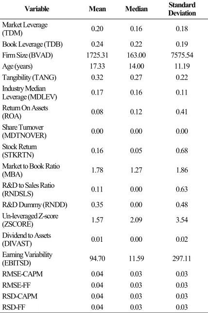
Table 1 reports the summary statistics of variables which we use and the definition of each variable. All of these variables are winsorized at 0.5% of both sides of the distribution to mitigate the impact of extreme observations and mis-recorded data.
Variables and Variables Definition
The dependent variable is leverage, measured using market leverage (TDM) and book leverage (TDB). Market leverage is ratio of total debt divided by market value of assets while book leverage is ratio of total debt divided by book value of assets.
The independent variables are slope of demand curve for stock and control variables. All explanatory variables are lagged one period. Proxy for the slope of demand curve for stock is idiosyncratic risk of stock returns which is measured using RMSE-CAPM, FF, RSD-CAPM, and RSD-FF.
RMSE-CAPM is root mean square error of residuals from a regression of daily excess returns on the market model. RMSE-FF is root mean square error of residuals from a regression of daily excess returns on
the Fama and French’ (1993) extended four-factor.
RSD-CAPM is standard deviation of the residuals from a regression of daily excess returns on the market model. RSD-FF is standard deviation of the residuals from a regression of daily excess returns on the Fama and French’ (1993) extended four-factor.
Control variables are size, age, tangibility, Industry median leverage, profitability, turnover, stock return, market to book ratio, research and development to sales ratio, research and development dummy, z-score, dividend to assets ratio, and earning’s variability. Firm size (LNBVAD1) is log of book value assets deflated by Consumer Price Index to account for inflation. Firm age (LNAGE1) is log of the firm’s age or number of years since the Initial Public Offering (IPO) year. Tangibility (TANG1) is the net property, plant, and equipments to asset ratio. Industry median leverage (MDLEV1) is the median of the ratio of total debt to the market value of assets by industry and by year. Return on Assets (ROA1), a profitability measurement, is the operating income before depreciation and amortization divided by total assets. Share turnover (MDTNOVER1), proxy for firm’s stock liquidity, is median value of monthly shares traded (volume) divided by shares outstanding over a twelve month period. Stock Return (STKRTN1) is compounded annual stock return over a twelve-month period, obtained from CRSP dataset. Market to Book Ratio (MBA1), well-known as proxy for growth opportunities, is market value of assets divided by book value of assets. Research and Development to Sales (RNDSLS1) is research and development expenses divided by net sales. Research and Development Dummy (RNDD1) is dummy variable which take value of one if firm does not have research and development expenses, zero otherwise. Altman Un-leveraged Z-score (ZSCORE1) is equals to [(3.3*pretax income + sales + 1.4*retained earnings + 1.2*(current assets – current liabilities))/ total assets]. Dividend to Assets Ratio (DIVAST1) is common stocks dividends divided by total assets. Earning’s Variability (EBITSD) is historical standard deviation of the ratio of EBITDA to total assets.
Summary Statistics
ratio in overall sample is 20% while book leverage ratio is 24%. The median of market leverage ratio and book leverage ratio are 16% and 22% respectively. Idiosyncratic volatility (proxy for the slope of demand curve for stock) as measured using RMSE-CAPM, RMSE-FF, RSD-CAPM, and RSD-FF has mean, median, and standard deviation of 4%, 3%, and 3% respectively. When four decimal points are used instead of two decimal points, we can see the slight difference of idiosyncratic volatility estimation using those various methods i.e. RMSE-CAPM, RMSE-FF, RSD-CAPM, and RSD-FF. However, the difference is trivial. Average age of firms listed in Compustat between 1971 and 2004 is 17.33 years. The minimum number of years per firm is 2, the maximum is 34, and the median is 14.
Table 1. Summary Statistics
Variable Mean Median Deviation Standard
Market Leverage
(TDM) 0.20 0.16 0.18
Book Leverage (TDB) 0.24 0.22 0.19 Firm Size (BVAD) 1725.31 163.00 7575.54 Age (years) 17.33 14.00 11.19 Tangibility (TANG) 0.32 0.27 0.22 Industry Median
Leverage (MDLEV) 0.17 0.16 0.11 Return On Assets
(ROA) 0.08 0.12 0.41
Share Turnover
(MDTNOVER) 0.00 0.00 0.00 Stock Return
(STKRTN) 0.16 0.05 0.68 Market to Book Ratio
(MBA) 1.78 1.27 1.86
R&D to Sales Ratio
(RNDSLS) 0.11 0.00 0.63 R&D Dummy (RNDD) 0.35 0.00 0.48 Un-leveraged Z-score
(ZSCORE) 1.57 2.09 3.54 Dividend to Assets
(DIVAST) 0.01 0.00 0.02 Earning Variability
(EBITSD) 94.70 11.59 297.11
RMSE-CAPM 0.04 0.03 0.03
RMSE-FF 0.04 0.03 0.03
RSD-CAPM 0.04 0.03 0.03
RSD-FF 0.04 0.03 0.03
Table 2 also displays the correlation coefficients between slope of demand curves and leverage. This univariate analysis shows that the slope of demand curve for stock (as shown by CAPM, RMSE-FF, RSD-CAPM, and RSD-FF) is positively related to the leverage ratio. Greater magnitude of RMSE-CAPM, RMSE-FF, RSD-RMSE-CAPM, and RSD-FF represent steeper demand curve for a firm’s stock. This preliminary evidence supports the idea that firms with steeper demand curve tend to have higher leverage ratio.
Pairwise correlation coefficients between control variables and leverage are reported in table 2 as well. Most correlation coefficients have expected signs. For instance, size and leverage are positively correlated. Tangibility and leverage are positively correlated suggesting that firms which have more tangible assets tend to have more leverage. The low correlations among independent variables indicate that one can include these variables in the same regressions without concerning about multicollinearity.
RESULTS AND ANALYSIS
Slope of Demand Curve for Stock and Actual Leverage Ratio
Actual Market Leverage
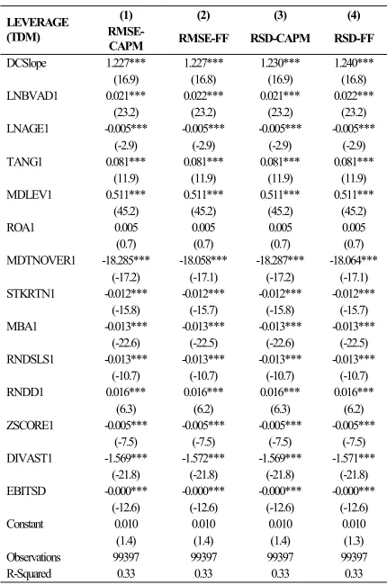
Table 3 presents the regression results of actual market leverage on the slope of demand curve for stock. Results show that there is positive and statistically significant relationship between the slope of demand curve for stock and actual market leverage and are consistent across various measurement methods of the slope of demand curve for stock (RMSE-CAPM, RMSE-FF, CAPM, and RSD-FF). Even after controlling for other factors shown in prior studies to influence leverage, the coefficient of the slope of demand curve for firm’s stock on firm’s actual market leverage is positive and statistically significant at 1% level demonstrating that firms with steeper slope of demand curves tend to have higher actual market leverage. This result also implies that the slope of demand curves for stock is an additional determinant factor in predicting firm’s market leverage.
Most control variables are significant and have the expected signs. For instance, firm size, tangibility, and industry median leverage are positively related to leverage. This is consistent with prior literatures (e.g. Harris and Raviv (1991), Frank and Goyal (2004)). Harris and Raviv (1991) document that larger firms have higher leverage. It is well known that firms with more tangible assets tend to have higher leverage as
they can pledge their assets in support of debt. Frank and Goyal (2004) find that industry leverage is prominent determinant of firm’s leverage, which is exactly what is found in this research. They provide explanation that firms in high leverage industry have higher leverage since firms in the same industry must face many common factors.
Table 3. Actual Market Leverage and the Slope of Demand Curve
(1) (2) (3) (4) LEVERAGE
(TDM)
RMSE-CAPM RMSE-FF RSD-CAPM RSD-FF
DCSlope 1.227*** 1.227*** 1.230*** 1.240***
(16.9) (16.8) (16.9) (16.8)
LNBVAD1 0.021*** 0.022*** 0.021*** 0.022***
(23.2) (23.2) (23.2) (23.2)
LNAGE1 -0.005*** -0.005*** -0.005*** -0.005***
(-2.9) (-2.9) (-2.9) (-2.9)
TANG1 0.081*** 0.081*** 0.081*** 0.081***
(11.9) (11.9) (11.9) (11.9)
MDLEV1 0.511*** 0.511*** 0.511*** 0.511***
(45.2) (45.2) (45.2) (45.2)
ROA1 0.005 0.005 0.005 0.005
(0.7) (0.7) (0.7) (0.7)
MDTNOVER1 -18.285*** -18.058*** -18.287*** -18.064***
(-17.2) (-17.1) (-17.2) (-17.1)
STKRTN1 -0.012*** -0.012*** -0.012*** -0.012***
(-15.8) (-15.7) (-15.8) (-15.7)
MBA1 -0.013*** -0.013*** -0.013*** -0.013***
(-22.6) (-22.5) (-22.6) (-22.5)
RNDSLS1 -0.013*** -0.013*** -0.013*** -0.013***
(-10.7) (-10.7) (-10.7) (-10.7)
RNDD1 0.016*** 0.016*** 0.016*** 0.016***
(6.3) (6.2) (6.3) (6.2)
ZSCORE1 -0.005*** -0.005*** -0.005*** -0.005***
(-7.5) (-7.5) (-7.5) (-7.5)
DIVAST1 -1.569*** -1.572*** -1.569*** -1.571***
(-21.8) (-21.8) (-21.8) (-21.8)
EBITSD -0.000*** -0.000*** -0.000*** -0.000***
(-12.6) (-12.6) (-12.6) (-12.6)
Constant 0.010 0.010 0.010 0.010
(1.4) (1.4) (1.4) (1.3)
Observations 99397 99397 99397 99397
R-Squared 0.33 0.33 0.33 0.33
good. In accordance with Frank and Goyal (2004), this paper finds that dividend paying firms tend to have lower leverage ratio.
Contrary to the view that mature firms typically have higher leverage because they have more reputation in debt markets hence can borrow at lower cost of debt, this research find that mature firms tend to borrow less. This probably because mature firms have more cash flow in the first place thus not only need less outside financing, but also tend to pay-off debt instead of borrows more. Firms with more liquid stocks tend to have less leverage. The liquidity of firm’s stocks suggests that firms can raise equity more easily and cheaply in the market because markets can absorb firm’s stocks in the event of equity issuance. The more liquid firms’ stocks, the more likely firms will issue equity hence the lower their leverage will be. Finally, as suggested by trade-off theory, firms react to risk by reducing leverage. In line with this view, this research paper finds that earnings variability (proxy for risk) is negatively related with leverage.
Actual Book Leverage
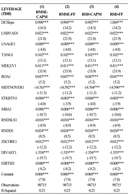
The regression of actual book leverage on various proxies of the slope of demand curve for stock is reported in table 4. When book leverage is used instead of market leverage, the same results are found. The slope of demand curves for stock is a positive and statistically significant factor in predicting book leverage of the firm, even though other variables shown to affect leverage had been controlled. Across various proxies of the slope of demand curve for stock (RMSE-CAPM, RMSE-FF, CAPM, and RSD-FF), the coefficient of the slope of demand curve for stock to the actual book leverage is positive and significant at 1% level suggesting that firms with steeper slope of demand curves have higher actual book leverage.
Other factors i.e. the control variables have same signs and magnitude as in market leverage regression. The only remarkable difference is that return on assets (ROA) as one of the profitability measures is a positive and statistically significant factor to explain book leverage while it is insignificant for market leverage. This is possibly because ROA as an accounting ratio, is based on book value and more backward looking which are features also shared by book leverage.
To sum up, the results from leverage regression show that slope of demand curve for stock has positive and significant effect on the firm’s actual leverage ratio (measured using either market or book
leverage), even after controlling for other factors which have been shown in past literatures to influence firm’s leverage. The results confirm the first hypothesis that firms with steeper demand curve for their stock suffer more from the share price drop if they issue equity hence are less likely to issue equity. Consequently, we will observe higher actual leverage ratio for these firms, which is exactly what is found from the empirical studies in this research.
Table 4. Actual Book Leverage and the Slope of Demand Curve
(1) (2) (3) (4) LEVERAGE
(TDB)
RMSE-CAPM RMSE-FF RSD-CAPM RSD-FF
DCSlope 0.990*** 0.994*** 0.992*** 1.004***
(14.3) (14.2) (14.3) (14.2)
LNBVAD1 0.022*** 0.022*** 0.022*** 0.022***
(21.8) (21.9) (21.8) (21.9)
LNAGE1 -0.009*** -0.009*** -0.009*** -0.009***
(-4.8) (-4.8) (-4.8) (-4.8)
TANG1 0.102*** 0.102*** 0.102*** 0.102***
(13.1) (13.1) (13.1) (13.1)
MDLEV1 0.411*** 0.411*** 0.411*** 0.411***
(33.9) (33.9) (33.9) (33.9)
ROA1 0.047*** 0.047*** 0.047*** 0.047***
(5.2) (5.2) (5.2) (5.2)
MDTNOVER1 -14.763*** -14.592*** -14.764*** -14.596***
(-11.3) (-11.2) (-11.3) (-11.2)
STKRTN1 -0.004*** -0.003*** -0.004*** -0.003***
(-4.0) (-3.9) (-4.0) (-3.9)
MBA1 -0.006*** -0.006*** -0.006*** -0.006***
(-10.7) (-10.6) (-10.7) (-10.6)
RNDSLS1 -0.016*** -0.016*** -0.016*** -0.016***
(-8.9) (-8.9) (-8.9) (-8.9)
RNDD1 0.024*** 0.024*** 0.024*** 0.024***
(8.5) (8.5) (8.5) (8.5)
ZSCORE1 -0.012*** -0.012*** -0.012*** -0.012***
(-12.2) (-12.2) (-12.2) (-12.2)
DIVAST1 -1.554*** -1.555*** -1.554*** -1.555***
(-19.7) (-19.7) (-19.7) (-19.7)
EBITSD -0.000*** -0.000*** -0.000*** -0.000***
(-8.2) (-8.2) (-8.2) (-8.2)
Constant 0.060*** 0.060*** 0.060*** 0.060***
(7.9) (7.9) (7.9) (7.8)
Observations 98715 98715 98715 98715
R-Squared 0.23 0.23 0.23 0.23
Slope of Demand Curve for Stock and Target Leverage Ratio
Target Market Leverage
one period market leverage ratio,
(
1
−
λ
)
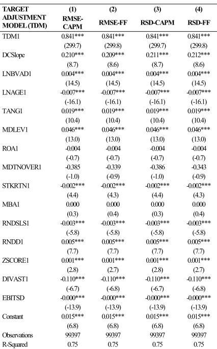
, we can infer how fast firms adjust their market leverage ratio to the estimated target market leverage ratio. The coefficient of the lagged market leverage is 0.841. It implies that firms close 15.9% (= 1 - 0.841) of the gap between current and target leverage within one year.Table 5. Target Market Leverage and the Slope of Demand Curve
(1) (2) (3) (4) TARGET
ADJUSTMENT MODEL (TDM)
RMSE-CAPM RMSE-FF RSD-CAPM RSD-FF
TDM1 0.841*** 0.841*** 0.841*** 0.841***
RNDD1 0.005*** 0.005*** 0.005*** 0.005***
(7.7) (7.7) (7.7) (7.7)
Observations 99397 99397 99397 99397
R-Squared 0.75 0.75 0.75 0.75
The coefficient of DCSlope to target market leverage ratio,
ϕ
, is also positive and significant. This result is consistent with Hypothesis 2 which states that firms with steeper demand curve tend to have higher target leverage ratios. We can also infer the coefficient of the slope of demand curve to the target market leverage ratio from the result. For instance, usingRMSE of Fama and French’s extended four-factor
model as proxy for the slope of demand curve, the coefficient of the slope of demand curve to market
leverage ratio,
ϕ
, is 0.209. Sinceϕ
=
λγ
, we candecompose them to find the impact of the slope of demand curve to the target market leverage ratio. We
know that
ϕ
is 0.209 andλ
is 0.159, hence we canfigure out that
γ
, the coefficient of demand curveslope to the target market leverage ratio, is 1.314. In
this case, we also found that the impact of the slope of demand curve to the target debt ratio is positive and significant which means that firms with steeper demand curve tend to have higher target market leverage ratio.
Other factors have expected sign and similar to the results found in the actual leverage regression. Note however, when lagged one period debt ratio of the firm is included in the regression, some significant explanatory variables in previous regressions (equation 6(a)), specifically stock’s liquidity and market to book ratio, are no longer significant.
Target Book Leverage
Table 6 presents target adjustment regression result using book leverage as the dependent variable. Essentially, using book leverage instead of market leverage in the model does not alter the main finding.
Lagged one period book leverage ratio (TDB1) has significant positive effect on the target book leverage ratio indicating that firms gradually adjust to the target leverage ratio. Similar to the result in target adjustment regression using market leverage, the coefficient on the lagged book leverage implies that firms close 15.9% (= 1 - 0.841) of the gap between current and target leverage within one year.
The slope of demand curve for stock also has significant positive effect on the target book leverage ratio, even though other factors shown to affect leverage and lagged one period book leverage ratio had been controlled. Using RMSE of Fama and
French’s extended four-factor model as proxy for the
slope of demand curve, the coefficient of the slope of
demand curve to book leverage ratio,
ϕ
, is 0.187.Since
ϕ
=
λγ
, we can decompose them to find theimpact of the slope of demand curve to the target
book leverage ratio. We know that
ϕ
is 0.187 andλ
is 0.159, hence we can figure out that
γ
, thecoefficient of demand curve slope to the target book leverage ratio is 1.176. The results support the second hypothesis which predicts that firms with steeper slope of demand curve tend to have higher target leverage ratio. The reason is because firms with a steeper slope of demand curve for their stock are less likely to issue equity since they will suffer more in the declining of their share price when they choose to do so.
liquidity, and market to book ratio, and Altman un-leveraged z-score are no longer significant.
Compared to market leverage target adjustment regression, one prominent difference is that the effect of Altman un-leveraged z-score on the book leverage is not significant while it is significant on the market leverage.
Table 6. Target Book Leverage and the Slope of Demand Curve
(1) (2) (3) (4)
TARGET ADJUSTMENT MODEL (TDB)
RMSE-CAPM RMSE-FF RSD-CAPM RSD-FF
TDB1 0.841*** 0.841*** 0.841*** 0.841***
(275.6) (275.6) (275.6) (275.6)
DCSlope 0.186*** 0.187*** 0.186*** 0.189***
(7.4) (7.4) (7.4) (7.4)
LNBVAD1 0.003*** 0.003*** 0.003*** 0.003***
(9.7) (9.8) (9.7) (9.8)
LNAGE1 -0.005*** -0.005*** -0.005*** -0.005***
(-9.5) (-9.5) (-9.5) (-9.5)
TANG1 0.019*** 0.019*** 0.019*** 0.019***
(9.5) (9.5) (9.5) (9.5)
MDLEV1 0.039*** 0.039*** 0.039*** 0.039***
(10.9) (10.9) (10.9) (10.9)
ROA1 -0.008 -0.008 -0.008 -0.008
(-1.6) (-1.6) (-1.6) (-1.6)
MDTNOVER1 0.176 0.208 0.176 0.205
(0.4) (0.5) (0.4) (0.5)
STKRTN1 -0.005*** -0.005*** -0.005*** -0.005***
(-7.9) (-7.9) (-7.9) (-7.9)
MBA1 -0.000 -0.000 -0.000 -0.000
(-1.3) (-1.2) (-1.3) (-1.2)
RNDSLS1 -0.002** -0.002* -0.002** -0.002*
(-2.0) (-2.0) (-2.0) (-2.0)
RNDD1 0.006*** 0.006*** 0.006*** 0.006***
(8.0) (8.0) (8.0) (8.0)
ZSCORE1 -0.000 -0.000 -0.000 -0.000
(-0.0) (-0.0) (-0.0) (-0.0)
DIVAST1 -0.087*** -0.087*** -0.087*** -0.087***
(-4.4) (-4.4) (-4.4) (-4.4)
EBITSD -0.000*** -0.000*** -0.000*** -0.000***
(-7.0) (-7.0) (-7.0) (-7.0)
Constant 0.022*** 0.022*** 0.022*** 0.022***
(8.7) (8.7) (8.7) (8.7)
Observations 98534 98534 98534 98534
R-Squared 0.73 0.73 0.73 0.73
To summarize, results from the target adjustment regression model demonstrate that downward sloping demand curve for stock has significant positive effect on the target leverage ratio which suggests that the steeper the slope of demand curve for firm’s stock, the higher the firm’s target leverage ratio. This result verifies Hypothesis 2 and holds regardless whether market leverage or book leverage is used. Lagged debt ratio in the target adjustment regression model is also positive and significant which indicates that firms gradually adjust to the target leverage ratio. It is found that the estimated adjustment speed to close the gap between firm’s actual leverage ratio and target leverage ratio is 15.9%.
CONCLUSIONS
This research paper empirically investigates the effect of downward sloping demand curves for stock on firms’ financing decisions. Downward sloping demand curves for stock implies that when firms issue equity (which can be seen as an increase in supply), the share price of issuing firms will decrease. The decline in the firm’s share price depends on the slope of demand curve. For the same amount of equity issuance, firms with a steeper slope of demand curve experience a larger price drop than firms with flatter demand curves. Therefore, ceteris paribus, it is argued that firms with steeper demand curves are less likely to issue equity and hence we should observe higher actual leverage ratios for these firms. To the extent that each firm has an optimal leverage ratio, these firms should also have higher target leverage ratios.
The main findings in this research paper provide supporting evidence on the proposed hypotheses. Results show that firms with steeper demand curves for stock have higher actual leverage ratios. Even after controlling for other factors which had been shown in prior studies to influence firms’ leverage, it is found that the slope of demand curves for stock positively and significantly affects a firm’s actual leverage. The results indicate that firms with steeper demand curves are more likely to choose debt than equity in order to avoid greater adverse price impact of equity issuance on their share price. Furthermore, firms’ target leverage ratios are higher for firms with steeper demand curves. Unlike actual leverage, firms’ target leverage is not directly observable. However, we can attain it using a target adjustment model. From the target adjustment regression, it can be seen that the slope of demand curve for stock is a positive, statistically significant factor for firms’ target leverage ratios suggesting that there are additional incentives for these firms to use debt financing.
REFERENCES
Amihud, Y., and H. Mendelson, 1986, Asset pricing
and the bid-ask spread, Journal of Financial
Economics 17, 223-249.
Baker, Malcolm P., Joshua Coval, and Jeremy C. Stein, 2006, Corporate financing decisions when investors take the path of least resistance,
Journal of Financial Economics, Forthcoming. Baker, Malcolm P., and Jeffrey Wurgler, 2002,
Market timing and capital structure, Journal of
Barclay, and Litzenberger, 1988, Announcement effects of new equity issues and the use of
intraday price data, Journal of Financial
Economics 21, 71-99.
Carhart, Mark M., 1997, On persistence in mutual
fund performance, Journal of Finance 52,
57-82.
Chang, Xin, Sudipto Dasgupta, and Gilles Hilary, 2006, Analyst coverage and financing decisions, Journal of Finance, Forthcoming. Chang, Xin, Sudipto Dasgupta, and Gilles Hilary,
2006, The effect of auditor choice on financing decisions, Working Paper.
Chang, Xin, Lewis Tam, Tek Jun Tan, and George Wong, 2006, The real impact of stock market
mispricing - evidence from Australia, Pacific
Basin Finance Journal, Forthcoming.
Cox, Nicholas J., 1998, WINSOR: Stata module to winsorize variable, Statistical Software Components S361402, Boston College Department of Economics, http://ideas.repec. org/c/boc/bocode/s361402.html
Diether, Karl B., Christopher J. Malloy, and Anna Scherbina, 2002, Differences of opinion and
the cross section of stock returns, Journal of
Finance 57, 2113-2141.
Fama, Eugene F., and Kenneth R. French, 1993, Common risk factors in the returns on stocks
and bonds, Journal of Financial Economics 33,
3-56.
Fama, Eugene F., and Kenneth R. French, 1996, Multifactor explanations of asset pricing anomalies, Journal of Finance 51, 55-84.
Fama, Eugene F., and Kenneth R. French, 2005, Financing decisions: Who issues stock?
Journal of Financial Economics 76, 549-582. Ferreira, Miguel A., and Paul A. Laux, 2005,
Corporate governance, idiosyncratic risk, and information flow, Working Paper, University of Delaware.
Flannery, Mark J., and Kasturi P. Rangan, 2004, Partial adjustment toward target capital structures, Working Paper, University of Florida.
Frank, Murray Z., and Vidhan K. Goyal, 2004, Capital structure decisions: Which factors are reliably important?, Working paper, UBC and HKUST.
Frank, Murray Z., and Vidhan K. Goyal, 2005, Tradeoff and pecking order theories of debt, in
B. Espen Eckbo, ed.: Handbook of Corporate
Finance: Empirical Corporate Finance. Graham, John R., and Campbell R. Harvey, 2001,
The theory and practice of corporate finance:
Evidence from the field, Journal of Financial
Economics 60, 187-243.
Haggard, K. Stephen, and Raynolde Pereira, 2005, Price pressure and the response to share repurchase announcements, Working Paper, University of Missouri-Columbia.
Harris, Milton, and Artur Raviv, 1991, The theory of
capital structure, Journal of Finance 46,
297-355
Hirt, Geoffrey, and G. S. Pandher, 2005, Idiosyncratic risk and return across S&P 500 stocks, Working Paper, DePaul University, Chicago, Illinois.
Holcombe, Randall G., and Richard P. Saba, 1984, The effects of heterogeneous expectations on
the capital structure of the firm, Southern
Economic Journal 51, 356-368.
Holthausen, Robert W., Richard W. Leftwich, and David Mayers, 1990, Large-block transactions, the speed of response, and temporary and
permanent stock-price effects, Journal of
Financial Economics 26, 71-95.
Hovakimian, Armen, Tim Opler, and Sheridan
Titman, 2001, The debt-equity choice, Journal
of Financial and Quantitative Analysis 36, 1-24.
Jegadeesh, Narasimhan, and Sheridan Titman, 1993, Returns to buying winners and selling losers: Implications for stock market efficiency,
Journal of Finance 48, 65-91.
Jegadeesh, Narasimhan, and Sheridan Titman, 2001, Profitability of momentum strategies: An
evaluation of alternative explanations, Journal
of Finance 56, 699-720.
Kamara, Avraham, 1994, Liquidity, taxes, and
short-term treasury yields, Journal of Financial and
Quantitative Analysis 29, 403-417.
Kaul, Aditya, Vikas Mehrotra, and Randall Morck, 2000, Demand curves for stocks do slope down: New evidence from an index weights
adjustment, Journal of Finance 55, 893-912.
Loderer, Claudio, John W. Cooney, and Leonard D. Van Drunen, 1991, The price elasticity of
demand for common stock, Journal of Finance
Marsh, Paul, 1982, The choice between equity and
debt: An empirical study, Journal of Finance
37, 121-144.
Masulis, Ronald W., 1980, The effect of capital structure change on security prices: A study of
exchange offers, Journal of Financial
Economics 8, 139-178.
Mayshar, J., 1978, Investors' time horizon and the
efficiency of capital markets, Quarterly
Journal of Economics 92, 187-208.
Merton, Robert C., 1987, A simple model of capital market equilibrium with incomplete
information, Journal of Finance 42, 483–510.
Mikkelson, Wayne H., and Megan Partch, 1985, Stock price effects and costs of secondary
distributions, Journal of Financial Economics
14, 165-194.
Miller, Edward, 1977, Risk, uncertainty, and
divergence of opinion, Journal of Finance 32,
1151-1168.
Myers, Stewart C., 1984, The capital structure puzzle,
Journal of Finance 39, 575-592.
Myers, Stewart C., 2001, Capital structure, Journal of
Economic Perspectives 15, 81-102.
Myers, Stewart C., and Nicholas S. Majluf, 1984, Corporate financing and investment decisions when firms have information that investors do
not have, Journal of Financial Economics 13,
187-221.
Parsons, John E., and Artur Raviv, 1985,
Underpricing of seasoned issues, Journal of
Financial Economics 14, 377-397.
Petajisto, Antti, 2004, Why do demand curves for stocks slope down?, Yale ICF Working Paper #04-06, Yale School of Management.
Scherbina, Anna, 2004, Analyst disagreement, forecast bias and stock returns, HBS Publishing, Forthcoming.
Scholes, Myron S., 1972, The market for securities: Substitution versus price pressure and the
effects of information on share prices, Journal
of Business 45, 179-211.
Shleifer, Andrei, 1986, Do demand curves for stocks
slope down?, Journal of Finance 41, 579-590.
Shleifer, Andrei, and Lawrence H. Summers, 1989, Crowds and prices: Toward a theory of inefficient markets, CRSP Working Paper Series #282, University of Chicago.
Shleifer, Andrei, and Robert W. Vishny, 1997, The
limits of arbitrage, Journal of Finance 52,
35-55.
Titman, Sheridan, 1984, The effect of capital structure
on a firm's liquidation decision, Journal of
Financial Economics 13, 137-151.
Warga, Arthur, 1992, Bond returns, liquidity, and
missing data, Journal of Financial and
Quantitative Analysis 27, 605-617.
Wurgler, Jeffrey, and Ekaterina Zhuravskaya, 2002, Does arbitrage flatten demand curves for stocks?, Journal of Business 75, 583-608. Yaffee, Robert A., 2002, Getting started with stata for
MS Windows: A brief introduction, New York University, www.nyu.edu/its/socsci/Docs/ Intro_ stata5.pdf
VARIABLES DEFINITION AND VARIABLES CONSTRUCTION
Market Value of Equity is defined as the number of shares outstanding multiplied by closing stock price at the end of the fiscal year (from CRSP).
Market Leverage (TDM) is ratio of total debt divided by market value of assets i.e. market value of equity plus total liability {(Compustat item 9 + Compustat item 34)/(market value of equity + (Compustat item 9 + Compustat item 34))}.
Book Leverage (TDB) is ratio of total debt divided by book value of assets {(Compustat item 9 + Compustat item 34)/Compustat item 6}.
Size (LNBVAD) is log of book value of assets deflated by Consumer Price Index to account for inflation {Compustat item number 6/Consumer Price Index}.
Age is the firm’s age measured as the number of years since the Initial Public Offering (IPO) year.
Tangibility (TANG) is the net property, plant, and equipments to asset ratio {Compustat item 8/Compustat item 6}.
Industry Median Leverage (MDLEV) is the median of the ratio of total debt to the market value of assets by three-digit SIC code and by year.
Median turnover (MDTNOVER), proxy for firm’s stock liquidity, is median value of monthly shares traded (volume) divided by shares outstanding over a twelve month period.
Annual Stock Return (STKRTN) is compounded annual stock return over a twelve-month period. Stock return is obtained from CRSP dataset.
Market-to-book ratio (MBA) is defined as market value of assets divided by total assets {(market value of equity + (Compustat item 9 + Compustat item 34))/Compustat item 6}.
R&D to Sales (RNDSLS) is research and develop-ment expenses to sales ratio {Compustat item 46/Compustat item 12}.
R&D Dummy (RNDD) is dummy variable which take value of one if research and development expense is missing, zero otherwise.
Altman’s Un-leveraged Z-score (ZSCORE) is obtained from (3.3*pretax income + sales + 1.4*retained earnings + 1.2*(current assets – current liabilities)) divided by total assets. {(3.3*Compustat item 178 + Compustat item 12 + 1.4*Compustat item 36 + 1.2*(Compustat item 4 – Compustat item 5))/Compustat item 6}.
DIVAST is common stocks dividends to assets ratio {Compustat item 21/Compustat item 6}.