Full Terms & Conditions of access and use can be found at
http://www.tandfonline.com/action/journalInformation?journalCode=ubes20
Download by: [Universitas Maritim Raja Ali Haji] Date: 12 January 2016, At: 23:23
Journal of Business & Economic Statistics
ISSN: 0735-0015 (Print) 1537-2707 (Online) Journal homepage: http://www.tandfonline.com/loi/ubes20
Idiosyncratic Volatility, Stock Market Volatility, and
Expected Stock Returns
Hui Guo & Robert Savickas
To cite this article: Hui Guo & Robert Savickas (2006) Idiosyncratic Volatility, Stock Market Volatility, and Expected Stock Returns, Journal of Business & Economic Statistics, 24:1, 43-56, DOI: 10.1198/073500105000000180
To link to this article: http://dx.doi.org/10.1198/073500105000000180
Published online: 01 Jan 2012.
Submit your article to this journal
Article views: 306
View related articles
Idiosyncratic Volatility, Stock Market Volatility,
and Expected Stock Returns
Hui G
UOResearch Division, Federal Reserve Bank of St. Louis, St. Louis, MO 63166 (hui.guo@stls.frb.org)
Robert S
AVICKASDepartment of Finance, George Washington University, Washington, DC 20052 (savickas@gwu.edu)
We find that the value-weighted idiosyncratic stock volatility and aggregate stock market volatility jointly exhibit strong predictive power for excess stock market returns. The stock market risk–return relation is found to be positive, as stipulated by the capital asset pricing model; however, idiosyncratic volatility is negatively related to future stock market returns. Also, idiosyncratic volatility appears to be a pervasive macrovariable, and its forecasting abilities are very similar to those of the consumption–wealth ratio proposed by Lettau and Ludvigson.
KEY WORDS: Consumption–wealth ratio; Dispersion of opinion; Intertemporal capital asset pricing model; Out-of-sample forecast; Stock market risk-return relation; Stock return pre-dictability.
1. INTRODUCTION
Early authors (e.g., Campbell 1987; Glosten, Jagannathan, and Runkle 1993; Whitelaw 1994) failed to uncover a posi-tive risk–return relation in the stock market across time, as dic-tated by the capital asset pricing model (CAPM). In this article we investigate whether their results reflect an omitted variables problem; in addition to stock market volatility, aggregate idio-syncratic volatility also may be an important determinant of the equity premium for at least three reasons. First, it is priced be-cause many investors hold poorly diversified portfolios (e.g., Levy 1978; Malkiel and Xu 2001). Second, it is a proxy for the divergence of opinion, which could lead a stock to be overval-ued initially and to subsequently suffer capital losses if short-sales constraints are binding (e.g., Miller 1977). Third, it tracks conditional stock market returns because, by construction, it measures the conditional variance of the risk factor(s) of a mul-tifactor or intertemporal capital asset pricing model (ICAPM) model omitted from the CAPM (e.g., Lehmann 1990).
We follow the early literature to construct the proxies for idiosyncratic volatility and stock market volatility. Similar to Campbell, Lettau, Malkiel, and Xu (2001) and Goyal and Santa-Clara (2003), we define realized value-weighted idiosyn-cratic volatility (IV) as
idiosyncratic shock to the excess return on stockiin day dof quartert. Following Merton (1980) and Andersen, Bollerslev, Diebold, and Labys (2003), for example, we define realized stock market volatility (MV) as
MVt= Dt
d=1
(emd−emd)2, (2)
whereemdis the excess stock market return in day d of
quar-ter t andemd is its quarterly average. Note that the volatility
measure in (2) is potentially downward-biased for two reasons. First, the quarterly average of the daily return is a noisy mea-sure of the expected daily return. Second, it does not account for the (positive) serial correlation in the daily stock market return. However, we find essentially the same results by (1) assuming that the expected daily return is equal to 0 and (2) adjusting for the serial correlation, as was done by French, Schwert, and Stambaugh (1987).
Over the period 1963:Q4–2002:Q4—the longest quarterly sample available to us at the time of writing—we find that, although IV and MV individually have negligible forecast-ing power in the in-sample regression, they jointly provide a significant predictor of excess stock market returns, with an adjusted R2 of >10%. We find very similar results using subsamples and alternative measures of IV. Moreover, their predictive abilities are also statistically significant in the out-of-sample tests. Therefore, as expected, the early authors failed to uncover a positive risk-return relation in the stock market possibly because of an omitted variables problem; IV is nega-tively related and MV posinega-tively related to future stock returns, whereas they are positively related to each other.
IV appears to be a pervasive macrovariable that captures sys-tematic movements of stock returns. For example, we form decile portfolios on past IV and find that aggregate IV is always significantly negative in the forecasting equation of portfolio returns and always drives out portfolio-specific IV. Similarly, aggregate IV also forecasts the value premium and returns on international stock market indices constructed by Morgan Stanley Capital International (MSCI). We also compare IV with the consumption–wealth ratio (CAY) proposed by Lettau and Ludvigson (2001), because, similar to IV, CAY is also found to help uncover a positive stock market risk–return relation (e.g.,
© 2006 American Statistical Association Journal of Business & Economic Statistics January 2006, Vol. 24, No. 1 DOI 10.1198/073500105000000180
43
Guo 2006). We find that IV is strongly (and negatively) corre-lated with CAY and that its forecasting abilities attenuate sub-stantially and vanish in some specifications if we control for CAY. Similarly, the predictive power of CAY becomes notice-ably weaker when combined with IV, although it remains sig-nificant in our sample. Therefore, IV and CAY capture similar predictable variations of stock market returns.
Finally, we compare IV with aggregate liquidity measures, which have systematic movements (e.g., Chordia, Roll, and Subrahmanyam 2000; Hasbrouck and Seppi 2001; Huberman and Halka 2001), are priced in the cross-section of stock re-turns (e.g., Pastor and Stambaugh 2003; Acharya and Pedersen 2005), and forecast stock market returns (e.g., Amihud 2002; Jones 2002). Interestingly, we find that IV and CAY both are highly correlated with, and have similar predictive abilities to, many commonly used liquidity measures, including trading volume, turnover, and bid–ask spread.
The negative relation between IV and conditional excess stock market returns contradicts the nondiversification hypoth-esis advocated by Levy (1978) and Malkiel and Xu (2001). It is consistent with the other two alternative hypotheses, how-ever. First, IV measures the conditional variance of an omitted risk factor, namely the liquidity risk, which, as argued by Guo (2004), could be negatively related to the stock market risk. Second, IV is a measure of the dispersion of opinion, which, as argued by Cao, Wang, and Zhang (2005), is positively related to stock market volatility but negatively related to conditional excess stock market returns. It should be noted that in these authors’ work, IV reflects a systematic risk factor of a multifac-tor or ICAPM model omitted from the CAPM. However, given that the dispersion of opinion is likely to be closely related to various liquidity measures considered in this article, the analy-sis does not allow us to distinguish between the two alternative hypotheses.
Our results differ from those of Goyal and Santa-Clara (2003), who found that conditional excess stock market returns are positively correlated with IV but are not correlated with MV. We attribute the differences to two factors. First, we focus most of our attention on the value-weighted IV, because we find that the equal-weighted measure (used by Goyal and Santa-Clara) forecasts stock returns mainly because of its co-movements with MV. Second, Ghysels, Santa-Clara, and Valkanov (2005) uncovered a positive stock market risk–return relation after tak-ing into account the effect of a long-distributed lag of returns on volatility. Therefore, IV and MV are likely to be more pre-cisely measured at the quarterly frequency used in this article than at the monthly frequency used by Goyal and Santa-Clara. Some recent authors (e.g., Scruggs 1998; Harrison and Zhang 1999; Guo and Whitelaw 2005) have also found that omitting the hedge component of Merton’s (1973) ICAPM introduces a downward bias in the stock market risk–return relation. More-over, Diether, Malloy, and Scherbina (2002), Easley, Hvidkjaer, and O’Hara (2002), and Ang, Hodrick, Xing, and Zhang (2005) have documented a cross-sectional negative relation between IV and expected returns.
The remainder of the article is organized as follows. We dis-cuss data in Section 2 and present the main results of forecasting stock market returns in Section 3. In Section 4 we investigate whether IV is a pervasive macrovariable and analyze its rela-tion to CAY and aggregate stock market liquidity. We provide concluding remarks in Section 5.
2. DATA
We use daily Center for Research on Security Prices (CRSP) stock files, which span July 1962–December 2002, to construct the IV defined in (1). There is ongoing debate about the CAPM. In particular, Fama and French (1993) argued that it should be augmented with two additional risk factors, SMB and HML, and showed that their three-factor (FF) model is quite success-ful in explaining the cross-section of stock returns. SMB is the return on a portfolio that is long in small stocks and short in big stocks, and HML is the return on a portfolio that is long in stocks with high book-to-market value ratios and short in stocks with low book-to-market value ratios. In this article we use the FF model to control for the systematic risk; however, we obtain very similar results using both the idiosyncratic shock based on the CAPM and the raw return. Campbell et al. (2001) docu-mented an upward deterministic trend in IV and found that it was more pronounced for small stocks than for big stocks. To mitigate the potential impact of this trend on our econometric inference, we construct IV using 500 stocks with the biggest market capitalization measured at the end of the previous quar-ter, although we find very similar results using all stocks in CRSP stock files.
The daily risk-free rate and the daily Fama and French three factors, which span July 1963–December 2002, were obtained from Kenneth French at Dartmouth College. The idiosyncratic shock,ηid, is thus the residual from the regression of the excess
return,erid—the difference between the return on stock iand
the risk-free rate—on the Fama and French three factors,fd,
erid=α+β·fd+ηid. (3)
Given that factor loadings,β, might change over time, we esti-mate (3) using a rolling sample. For example, the idiosyncratic shock at time d is equal to erid− ˆα− ˆβ·fd, where we
ob-tain the coefficient estimatesαˆ andβˆ using the daily data from d−130 tod−1. We require a minimum of 45 daily observa-tions to obtain less-noisy parameter estimates. Similar to Goyal and Santa-Clara (2003), we exclude stocks that have<15 re-turn observations in a quarter and drop the term 2Dit
d=2ridrid−1 stocks for which the market capitalization data at the end of the previous quarter are missing.
We use the difference between daily CRSP value-weighted stock market returns and the daily risk-free rate to construct MV, as defined in (2). It is important to note that the Octo-ber 19, 1987 stock market crash has a confounding effect on our measure of stock market volatility; realized volatility is 6.9% in 1987:Q4, compared with the second-largest realization of 2.7% in our sample. Schwert (1990) found that the behavior of realized volatility around the crash is unusual in many ways. Seyhun (1990) argued that the crash is not explained by the fundamentals. Hong and Stein (2003) suggested that the large fluctuations in stock prices immediately after the crash repre-sented a working out of microstructural distortions created on that chaotic day (e.g., jammed phone lines, overwhelmed mar-ket makers, unexecuted orders). To minimize the outlier effect of the 1987 crash, we follow Campbell et al. (2001) and many others and replace the realized volatility of 1987:Q4 with the second-largest observation in the sample. Nevertheless, we find
Figure 1. Idiosyncratic Volatility ( ——) and Stock Market Volatility ( - - - - -).
qualitatively the same results using the raw measure of MV, es-pecially if we add a dummy variable for the crash or take a log transformation to mitigate its impact; our results are robust to alternative treatments of the crash.
The monthly excess stock market returns (ER) is the differ-ence between the monthly CRSP value-weighted stock market return and the monthly CRSP risk-free rate. We aggregate the monthly excess return into quarterly data through geometric compounding. We obtained CAY from Martin Lettau at New York University. We also find that the stochastically detrended risk-free rate (RREL)—the difference between the risk-free rate and its average over the past 12 months—provides additional information about future stock returns beyond MV and IV. However, our results are not sensitive to whether we include it in the forecasting equation or not.
Figure 1 plots IV (solid line), with the shaded areas indicat-ing business recessions dated by the National Bureau of Eco-nomic Research (NBER). We note that IV rose dramatically in the late 1990s; we discuss the effect of this unusual episode on our results later in the article. Consistent with findings of Campbell et al. (2001) and many others, IV tends to rise dur-ing business recessions and exhibits an upward trend. We re-port the ordinary least squares (OLS) regression results of IV on constant and linear time trends, with the heteroscedasticity-correctedtstatistics in parentheses. Although a formal investi-gation is beyond the scope of this article, our preliminary results confirm those of Campbell et al. (2001) that the linear time trend accounts for substantial variations of IV. (Xu and Malkiel 2003 and Wei and Zhang 2006, among others, have provided some rationales for the upward trend in idiosyncratic volatility.) These variations are as follows:
IVt=C + t + εt, adjustedR2is .241. (4)
.007 .126E−03 (5.792) (5.609)
Given that the deterministic trend might lead to spurious re-gressions, for robustness we also report the results using the detrended idiosyncratic volatility (D_IV), which is the residual term of (4). For comparison, we also plot MV (dashed line) in Figure 1, which is substantially smaller than IV. The two series move closely with one another, but the correlation is not perfect. Interestingly, as shown in Figure 2, IV (solid line) also moves closely with CAY (dashed line) but in the opposite direction.
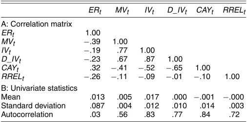
Table 1 provides summary statistics of the main variables used in this article. Consistent with the visual inspection from Figures 1 and 2, IV is positively correlated with MV and is neg-atively correlated with CAY, with correlation coefficients of .77
Figure 2. Idiosyncratic Volatility ( ——) and the Consumption–Wealth Ratio ( - - - - -).
and−.52. The correlation is .67 (−.65) between D_IV and MV (CAY). IV and D_IV are relatively persistent, with the autocor-relation coefficients of .83 and .77, compared with .56 for MV.
3. FORECASTING EXCESS STOCK
MARKET RETURNS
3.1 In-Sample Forecasting Regressions
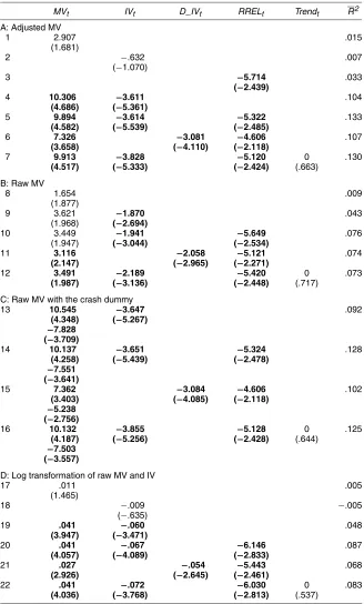
Table 2 presents the OLS regression results using IV and MV as forecasting variables for excess stock market returns. Over the full sample period 1963:Q4–2002:Q4 (panel A), we find that, individually, MV is positively related (row 1) and IV is negatively related (row 2) to future excess stock market returns, but neither variable is statistically significant at the 5% level. However, the two variables jointly are highly significant in the forecasting equation, with an adjusted R2 of >10% (row 4). These results may likely be explained by a classic omitted vari-ables problem: Whereas IV is negatively related and MV is positively related to future stock returns, the two variables are positively related to one another, as shown in Table 1. For il-lustration, we recall the omitted variables bias as exposited by, for example, Greene (1997, p. 402). Suppose that ER is the dependent variable, IV is the omitted variable with the true pa-rameter,γ1, and MV is the included variable with the true pa-rameter,γ2. Then the point estimate of the coefficient of MV is equal to γˆ2=γ2+covvar(MV(MV,IV))γ1. Given that γ1 is negative and cov(MV,IV)is positive, the point estimate,γˆ2, is thus bi-ased downward toward 0. This example indicates that the early authors failed to find a positive risk–return relation possibly be-cause of an omitted variables problem.
Table 1. Summary Statistics, 1963:Q4–2002:Q4
ERt MVt IVt D_IVt CAYt RRELt
A: Correlation matrix
ERt 1.00
MVt −.39 1.00
IVt −.19 .77 1.00
D_IVt −.23 .67 .87 1.00
CAYt .32 −.41 −.52 −.65 1.00
RRELt −.26 −.11 −.09 −.01 −.10 1.00 B: Univariate statistics
Mean .013 .005 .017 .000 −.001 −.000 Standard deviation .087 .004 .012 .010 .014 .003 Autocorrelation .03 .56 .83 .77 .84 .72
NOTE: We report summary statistics for excess stock market return,ERt; stock market volatil-ity,MVt; idiosyncratic volatility,IVt; detrended idiosyncratic volatility,D_IVt; the consumption– wealth ratio,CAYt; and the stochastically detrended risk-free rate,RRELt. To constructIVt, we use the FF model to control for the systematic risk and use only the largest 500 stocks in the CRSP stock files.
Table 2. Forecasting Quarterly Excess Stock Market Returns, Full Sample
MVt IVt D_IVt RRELt Trendt R2
A: Adjusted MV
1 2.907 .015
(1.681)
2 −.632 .007
(−1.070)
3 −5.714 .033
(−2.439)
4 10.306 −3.611 .104
(4.686) (−5.361)
5 9.894 −3.614 −5.322 .133
(4.582) (−5.539) (−2.485)
6 7.326 −3.081 −4.606 .107
(3.658) (−4.110) (−2.118)
7 9.913 −3.828 −5.120 0 .130
(4.517) (−5.333) (−2.424) (.663)
B: Raw MV
8 1.654 .009
(1.877)
9 3.621 −1.870 .043
(1.968) (−2.694)
10 3.449 −1.941 −5.649 .076
(1.947) (−3.044) (−2.534)
11 3.116 −2.058 −5.121 .074
(2.147) (−2.965) (−2.271)
12 3.491 −2.189 −5.420 0 .073
(1.987) (−3.136) (−2.448) (.717)
C: Raw MV with the crash dummy
13 10.545 −3.647 .092
(4.348) (−5.267) −7.828
(−3.709)
14 10.137 −3.651 −5.324 .128
(4.258) (−5.439) (−2.478)
−7.551 (−3.641)
15 7.362 −3.084 −4.606 .102
(3.403) (−4.085) (−2.118)
−5.238 (−2.756)
16 10.132 −3.855 −5.128 0 .125
(4.187) (−5.256) (−2.428) (.644)
−7.503 (−3.557)
D: Log transformation of raw MV and IV
17 .011 .005
(1.465)
18 −.009 −.005
(−.635)
19 .041 −.060 .048
(3.947) (−3.471)
20 .041 −.067 −6.146 .087
(4.057) (−4.089) (−2.833)
21 .027 −.054 −5.443 .068
(2.926) (−2.645) (−2.461)
22 .041 −.072 −6.030 0 .083
(4.036) (−3.768) (−2.813) (.537)
NOTE: We report the OLS regression results of the one-quarter-ahead excess stock market return on some predetermined variables. The heteroscadesticity-correctedtstatistics are in parentheses, and bold denotes significance at the 5% level.
MVtis stock market volatility;IVtis idiosyncratic volatility;D_IVtis detrended realized idiosyncratic volatility;RRELtis the stochastically detrended risk-free rate, andTrendtis a linear time trend. We make a downward adjustment for MV of 1987:Q4 in panel A and use the raw MV in panels B, C, and D. We include an additional variable in panel C, the product of MV with a dummy variable, which is equal to 1 for 1987:Q4 and 0 otherwise. The column MV has four numbers in panel C: The top (bottom) two numbers are point estimate andtvalue, for MV (the 1987:Q4 dummy). We use log transformation of IV and MV in panel D. The sample spans from 1963:Q4 to 2002:Q4.
The results in panel A of Table 2 cannot be explained by the spurious regressions stressed by Ferson, Sarkissian, and Simin (2003). First, the autocorrelations are .83 for IV and .56 for MV (Table 1). Therefore, our forecasting variables are not as persis-tent as most of the forecasting variables considered by Ferson
et al. Second, the absolute values oft statistics are 4.686 for MV and 5.361 for IV, in row 4 of Table 2. These numbers are substantially higher than the empirical criticaltvalues reported in table II of Ferson et al. for all cases, with only one excep-tion: Thetvalue for MV is slightly lower than 4.9—the case
in which the adjustedR2is .15 and the autocorrelation of pre-dictors is .99. But the autocorrelation of our prepre-dictors is much smaller than .99, as shown in Table 1. Also, Lanne (2002) found no evidence that expected stock market returns follow such a persistent process. Third, and more important, as we show in Section 3.4, IV and MV also exhibit statistically significant out-of-sample predictive abilities for stock market returns.
As discussed in Section 1, our forecasting variables are the-oretically motivated and thus are not subject to the criticism of data mining. It is also comforting to note that t statistics of IV and MV are still larger than the critical values for the cases of≤25 predictors in table III of Ferson et al. (2003), in which those authors considered the case of spurious regression jointly with data mining. Of course, the critical values in their table III would reject any forecasting model, including “the cor-rect model” that they considered, if we assume that the docu-mented predictability is based on a substantial degree of data mining. Moreover, there are ways to deal with data mining, such as using theoretically motivated variables and conducting out-of-sample forecast, as in our article.
Another potential issue is multicollinearity. MV and IV are closely correlated, as shown in Table 1. However, multi-collinearity cannot explain our results, because it usually leads to smalltstatistics, in contrast with the sharp increase oft sta-tistics from rows 1 and 2 to row 4 in Table 2. Moreover, the characteristic-root-ratio test proposed by Belsley, Kuh, and Welsch (1980) confirms that multicollinearity is unlikely to plague our results.
It is possible that IV forecasts stock market returns be-cause it is correlated with some commonly used predictive vari-ables. For example, consistent with findings of Campbell, Lo, and MacKinlay (1997) and others, RREL has some predictive power for stock returns (row 3). However, adding RREL to the forecasting equation has little effect on the forecasting abilities of IV and MV (row 5). Moreover, IV and MV drive out many other macrovariables (i.e., dividend yield, term premium, and default premium) from the forecasting equation. To conserve space, we do not report these results here, but they are available on request.
The deterministic trend in IV might bias our econometric in-ference. To address this issue, we consider two additional spec-ifications: using D_IV in row 6 and adding a linear time trend to the forecasting equation in row 7. In both cases, we obtain essentially the same results as those in row 5.
In panel A of Table 2, we made an ad hoc downward ad-justment for MV in 1987:Q4. To be robust, we repeat the fore-going analysis using unadjusted MV and report the results in panel B of Table 2. Again, we find that IV is always nega-tive and highly significant, whereas MV is always posinega-tive and significant or marginally significant. Although we obtain qual-itatively the same results using unadjusted MV, the predictive abilities are noticeably weaker than those reported in panel A of Table 2. To further investigate the potential effect of the 1987 crash, we include an additional variable—the product of MV with a dummy variable, which is equal to 1 for 1987:Q4 and 0 otherwise. We report the results in panel C of Table 2. The column MV now has four numbers for each specification. The top (bottom) two numbers are point estimate and t value, re-spectively, for MV (the 1987 crash dummy). We find that the
1987 crash dummy is always negative and statistically signifi-cant, confirming that the 1987 crash has a confounding effect on realized volatility. However, the sum of two slope parame-ters associated with MV is always positive, indicating that MV has an overall positive effect on expected stock returns imme-diately after the crash. Moreover, we find that the other results are almost identical to those reported in panel A of Table 2.
Finally, in panel D of Table 2 we report the estimation re-sults using transformed MV and IV. As expected, the log-transformation substantially mitigates the effect of potential outliers, and we obtain very similar results to those in panel A of Table 2. Overall, our results indicate that the 1987 crash has a confounding effect on realized volatility and thus must be ad-justed for. Nevertheless, our results are not sensitive to the par-ticular choice of adjustment—that is, adjusting MV of 1987:Q4 downward, adding a dummy variable for 1987:Q4, or using a log-transformation. To conserve space, we report only the re-sults obtained from using adjusted MV in the remainder of the article.
3.2 Subsamples
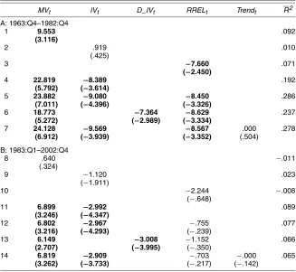
As shown in Figure 1, IV rose dramatically in the late 1990s until the stock market correction in the early 2000s. To inves-tigate whether this episode has any particular influence on the negative relation between IV and expected stock returns docu-mented in Table 2, we repeat our analysis using two subsam-ples and report the results in Table 3 for 1963:Q4–1982:Q4 (panel A) and 1983:Q1–2002:Q4 (panel B). In the first subsam-ple, we find that, consistent with the full samsubsam-ple, adding IV to the forecasting equation substantially improves the predictive ability of MV (row 4). We obtain the same results if we use D_IV in place of IV (row 6) or add a linear time trend to the forecasting equation (row 7). The results for the second sub-sample reported in panel B are also very similar to those for the full sample. Such a stable forecasting relation across time ex-plains the good out-of-sample performance, which we discuss in Section 3.4. However, there are two noticeable differences between two subsamples. First, the adjusted R2 much higher in panel A than in panel B. This result is consistent with that reported by Pesaran and Timmermann (1995), among others, who showed that predictable variations of stock returns change over time. Second, RREL becomes insignificant in the second subsample. However, this result is sensitive to the observations of 2001–2002, during which both the short-term rate and stock market prices fell steeply.
3.3 Alternative Measures of Idiosyncratic
Stock Volatility
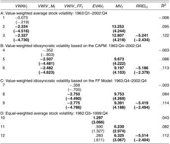
To investigate whether the results of Table 2 are sensitive to the particular measure of IV, we use various alternative mea-sures of IV to forecast excess stock market returns. We report the results in Table 4. Unless otherwise indicated, we calcu-late idiosyncratic stock volatility using all CRSP stocks through value-weighting. In panel A we use the raw stock return in (1) to calculate the average stock volatility (VWAV), which is ap-proximately the sum of IV and MV. We use only the market factor to control for the systematic risk in panel B (VWIV_M)
Table 3. Forecasting Quarterly Excess Stock Market Returns, Subsamples
MVt IVt D_IVt RRELt Trendt R2
A: 1963:Q4–1982:Q4
1 9.553 .092
(3.116)
2 .919 .010
(.425)
3 −7.660 .071
(−2.450)
4 22.819 −8.389 .192
(5.792) (−3.614)
5 23.882 −9.080 −8.450 .286
(7.011) (−4.396) (−3.326)
6 18.773 −7.364 −8.629 .237
(5.272) (−2.989) (−3.334)
7 24.128 −9.569 −8.567 .000 .278
(6.912) (−3.939) (−3.352) (.504)
B: 1983:Q1–2002:Q4
8 .640 −.011
(.324)
9 −1.120 .023
(−1.911)
10 −2.244 −.008
(−.648)
11 6.899 −2.992 .089
(3.246) (−4.347)
12 6.802 −2.967 −.755 .077
(3.216) (−4.293) (−.239)
13 6.149 −3.008 −1.152 .066
(2.707) (−3.995) (−.350)
14 6.819 −2.909 −.703 −.000 .065
(3.262) (−3.733) (−.217) (−.142)
NOTE: We report the OLS regression results of the one-quarter-ahead excess stock market return on some predeter-mined variables. The heteroscadesticity-correctedtstatistics are in parentheses, and bold denotes significance at the 5% level.MVtis stock market volatility,IVtis idiosyncratic volatility,D_IVtis detrended idiosyncratic volatility,RRELtis the stochastically detrended risk-free rate, andTrendtis a linear time trend.
and use the FF model in panel C (VWIV_FF). All three panels report results very similar to those in Table 2. Therefore, our re-sults are not sensitive to alternative measures of IV and, we use IV constructed from the 500 biggest stocks in the remainder of the article.
For comparison, in panel D we also present the results of the equal-weightedaverage stock volatility (EWAV) used by Goyal and Santa-Clara (2003). We follow these authors’ exact proce-dure and calculate EWAV on a monthly basis. We then use the EWAV of the last month in each quarter to forecast one-quarter-ahead stock returns over the sample period 1962:Q4–1999:Q4. We replicate their main result in row 10; EWAV is positive and highly significant in the forecasting regression, with an adjusted R2 of >4%. However, EWAV becomes insignificant after we include MV in the forecasting equation, whereas MV is signif-icantly positive (row 11). This result is not sensitive to whether we also add RREL to the forecasting equation (row 12). There-fore, the EWAV proposed by Goyal and Santa-Clara forecasts stock returns mainly because of its co-movements with stock market volatility.
3.4 Tests of Out-of-Sample Forecast Performance
Some recent authors (e.g., Bossaerts and Hillion 1999; Goyal and Welch 2003) have casted doubt on the in-sample evidence of stock return predictability, because they found that the pre-dictive variables used by the early authors did not forecast stock returns out of sample. However, Inoue and Kilian (2004) argued
that although out-of-sample tests are not necessarily more re-liable than in-sample tests, in-sample tests are more powerful than out-of-sample tests, even asymptotically. To address this issue, we use three statistics to compare the out-of-sample per-formance of our forecasting models with a benchmark of con-stant excess stock returns. First is the commonly used mean squared forecasting error (MSE) ratio. Second is Clark and McCracken’s (2001) encompassing test (ENC–NEW), which tests the null hypothesis that the benchmark model incorporates all of the information about the next quarter’s excess stock mar-ket return against the alternative hypothesis that our forecasting variables provide additional information. Third is McCracken’s (1999) equal forecast accuracy test (MSE–F), in which the null hypothesis is that the benchmark model has a MSE less than or equal to that of the augmented model and the alternative hy-pothesis is that the augmented model has a smaller MSE. Clark and McCracken (2001) showed that the latter two tests have the best overall power and size properties among the various tests proposed in the literature.
We report the results of the out-of-sample forecast tests in Table 5. Following Lettau and Ludvigson (2001), we use the first one-third of the observations for the initial in-sample es-timation and form the out-of-sample forecasts recursively in the remaining sample. That is, we use the observations over the period 1963:Q4–1976:Q4 to make the forecast for 1977:Q1 and update the sample to 1977:Q1 to forecast the return for 1977:Q2 and so forth. Note that we also estimate the expected return in the benchmark model recursively using the return data
Table 4. Alternative Measures of Idiosyncratic Volatility
VWAVt VWIV _Mt VWIV _FFt EVAVt MVt RRELt R2
A: Value-weighted average stock volatility: 1963:Q1–2002:Q4
1 −0.073 −.006
(−.219)
2 −2.334 13.253 .095
(−4.516) (4.244)
3 −2.327 12.807 −5.241 .122
(−4.730) (4.218) (−2.434)
B: Value-weighted idiosyncratic volatility based on the CAPM: 1963:Q4–2002:Q4
4 −.352 −.003
(−.803)
5 −2.507 9.673 .086
(−4.481) (4.222)
6 −2.482 9.197 −5.186 .113
(−4.623) (4.103) (−2.379)
C: Value-weighted idiosyncratic volatility based on the FF Model: 1963:Q4–2002:Q4
7 −.358 −.003
(−.705)
8 −2.750 9.753 .084
(−4.490) (4.269)
9 −2.775 9.391 −5.419 .114
(−4.786) (4.188) (−2.494) D: Equal-weighted average stock volatility: 1962:Q3–1999:Q4
10 1.297 .043
(3.066)
11 .590 6.230 .082
(1.327) (2.974)
12 .283 6.325 −5.514 .112
(.611) (3.067) (−2.404)
NOTE: We report the OLS regression results of the one-quarter-ahead excess stock market return on various alternative mea-sures of idiosyncratic volatility. The heteroscadesticity-correctedtstatistics are in parentheses, and bold denotes significance at the 5% level. Unless otherwise indicated, we calculate idiosyncratic volatility using all CRSP stocks through value weighting. We use the raw return in (1) to calculate average stock volatility,VWAVt(panel A), the idiosyncratic shock based on the CAPM for VWIV_Mt(panel B), and idiosyncratic volatility based on the FF model forVWIV_FFt(panel C).EVAVtis the monthly equal-weighted average stock volatility used by Goyal and Santa-Clara (2003). We convertEVAVtinto the quarterly data by taking only the last month’s observation for each quarter.MVtis stock market volatility, andRRELtis the stochastically detrended risk-free rate.
available at the time of forecast. The columnMSEA/MSEB is
the MSE ratio of the augmented model to that of the bench-mark model. The column “Asy. CV” reports the 95% critical value from the asymptotic distribution provided by Clark and McCracken (2001) and McCracken (1999), and the column “BS. CV” is the 95% critical value obtained from bootstrap-ping, as was done by Lettau and Ludvigson (2001). We use IV and MV as forecasting variables in row 1. Consistent with the in-sample regression results, we find that the augmented model has smaller MSE than the benchmark model of con-stant stock returns. More important, both the ENC–NEW and
MSE–F tests reject the null hypothesis that MV and IV provide no information about future stock returns at the 5% significance level using both asymptotic and bootstrapping critical values. For comparison, we also add RREL to the forecasting equation (row 2), and find that the results are mixed. Whereas the aug-mented model has negligible out-of-sample forecasting power according to the MSE ratio and the MSE–F test, the ENC–NEW test indicates that its predictive power is statistically signifi-cant at the 5% level. These results might reflect the structural break in the predictive power of RREL, as documented in Ta-ble 3.
Table 5. Tests of Out-of-Sample Forecast Performance
ENC–NEW MSE–F
Models MSEA/MSEB Statistic Asy. CV BS. CV Statistic Asy. CV BS. CV
1 C+MVt+IVtversusC .98 16.97 2.09 3.14 2.19 1.52 1.29 2 C+MVt+IVt+RRELtversusC 1.04 20.89 3.56 3.69 −3.52 1.61 .96
NOTE: We assume that excess stock market returns are constant in the benchmark model and augment the benchmark model withMVtandIVtin row 1 and withMVt,IVt, RRELtin row 2.MVtis stock market volatility,IVtis idiosyncratic volatility, andRRELtis the stochastically detrended risk-free rate. We report three out-of-sample forecast tests: (1) the mean-squared forecasting error (MSE) ratio of the augmented model to the benchmark model,MSEA/MSEB; (2) the encompassing test ENC–NEW developed by Clark and McCracken (2001); and (3) the equal forecast accuracy test MSE–F developed by McCracken (1999). ENC–NEW tests the null hypothesis that the benchmark model encompasses all the relevant information about the next quarter’s excess stock market return, against the alternative hypothesis that the predetermined variables provide additional information. MSE–F tests the null hypothesis that the benchmark model has a MSE less than or equal to the augmented model, against the alternative hypothesis that the augmented model has smaller MSE. We use observations over the period 1963:Q4–1976:Q4 for the initial in-sample estimation and then generate forecasts recursively for stock returns over the period 1977:Q1–2002:Q4. The “Asy. CV” column reports the asymptotic 95% critical values provided by Clark and McCracken (2001) and McCracken (1999). The “BS. CV” column reports the empirical 95% critical values obtained from the bootstrapping, as was done by Lettau and Ludvigson (2001). In particular, we first estimate a VAR(1) process of excess stock market returns and its forecasting variables with the restrictions under the null hypothesis. We then feed the saved residuals with replacements to the estimated VAR system, of which we set the initial values to their unconditional means. The ENC–NEW and MSE–F statistics are calculated using the simulated data, and the whole process is repeated 10,000 times.
Figure 3. Recursive MSE Ratio of Augmented Model to Benchmark Model (Table 5).
Figure 3 plots the recursive MSE ratio of the augmented model (row 1 of Table 5) to the benchmark model of con-stant returns through time. The horizontal axis denotes the starting forecast date; for example, the value corresponding to March 1976 is the MSE ratio over the forecast period 1976:Q1– 2002:Q4. We choose the range 1968:Q4–1997:Q4 for the start-ing forecast date; therefore, we use at least 20 observations for both the in-sample estimation and the calculation of MSE. As shown in Figure 3, except for a few years in the 1980s, the MSE ratio is always<1, indicating that IV and MV jointly have strong out-of-sample forecasting power for stock returns. We find very similar results for the MSE–F test, which is closely related to the MSE ratio. Interestingly, the ENC–NEW test in-dicates that the performance of the augmented model is always significantly better than that of the benchmark model at the 5% level.
4. IS IV A PERVASIVE MACROVARIABLE?
In the preceding section, we documented a negative relation between IV and conditional excess stock market returns. This result is somewhat puzzling, because it contradicts the nondi-versification hypothesis advocated by Levy (1978) and Malkiel
and Xu (2001), among others. However, as mentioned in Sec-tion 1, it appears to be consistent with equilibrium models (e.g., Guo 2004; Cao et al. 2005). In this section we further investi-gate whether, as suggested by these economic theories, IV is a pervasive macrovariable that captures systematic movements in stock returns.
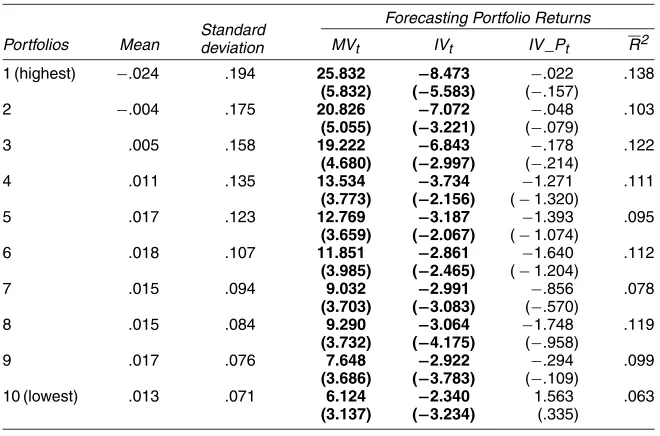
4.1 Forecasting Excess Returns on Portfolios
Formed on IV
We sort all CRSP stocks into decile portfolios by their real-ized IV in the past quarter; for example, stocks with the highest IV are in the first decile, and so forth. For each decile portfo-lio, we also calculate portfolio-specific idiosyncratic volatility (IV_P), using all stocks in that portfolio. Table 6 shows that, consistent with findings of Ang et al. (2005), the average re-turn is much lower for the portfolio of stocks with the highest IV (decile 1) than the portfolio of stocks with the lowest IV (decile 10). Also, the standard deviation of the portfolio return decreases monotonically from decile 1 to decile 10. We run a regression of the portfolio returns on MV, IV, and IV_P and re-port the OLS estimation results in the right part of Table 6. We have also controlled for RREL and a linear time trend in the forecasting equation; to conserve space, we do not report their point estimates. Also note that we obtain essentially the same results without these controls. For all 10 portfolios, IV_P is al-ways insignificant, whereas IV is alal-ways significant and neg-ative. These results indicate that aggregate IV is a pervasive macrovariable.
4.2 Forecasting Value Premium, Size Premium,
and Momentum Profit
Fama and French (1993) showed that the CAPM cannot ex-plain the value premium, HML, and the size premium, SMB.
Table 6. Forecasting Excess Returns on Portfolios Sorted by Past Idiosyncratic Volatility
Standard deviation
Forecasting Portfolio Returns
Portfolios Mean MVt IVt IV _Pt R2
1 (highest) −.024 .194 25.832 −8.473 −.022 .138 (5.832) (−5.583) (−.157)
2 −.004 .175 20.826 −7.072 −.048 .103
(5.055) (−3.221) (−.079)
3 .005 .158 19.222 −6.843 −.178 .122
(4.680) (−2.997) (−.214)
4 .011 .135 13.534 −3.734 −1.271 .111
(3.773) (−2.156) (−1.320)
5 .017 .123 12.769 −3.187 −1.393 .095
(3.659) (−2.067) (−1.074)
6 .018 .107 11.851 −2.861 −1.640 .112
(3.985) (−2.465) (−1.204)
7 .015 .094 9.032 −2.991 −.856 .078
(3.703) (−3.083) (−.570)
8 .015 .084 9.290 −3.064 −1.748 .119
(3.732) (−4.175) (−.958)
9 .017 .076 7.648 −2.922 −.294 .099
(3.686) (−3.783) (−.109)
10 (lowest) .013 .071 6.124 −2.340 1.563 .063 (3.137) (−3.234) (.335)
NOTE: We sort CRSP stocks into decile portfolios by their realized idiosyncratic volatility in the past quarter. For example, the first decile is the portfolio of stocks with the highest idiosyncratic volatility and so forth. The heteroscedasticity-corrected
tstatistics are in parentheses, and bold denotes significance at the 5% level.MVtis stock market volatility,IVtis idiosyncratic volatility, andIV_Ptis the portfolio-specific idiosyncratic volatility. We also control for the stochastically detrended risk-free rate,RRELt, and a linear time trend in the forecasting equation. The sample spans 1963:Q4–2002:Q4.
Fama and French (1996) also found that the existing asset pric-ing models fail to explain Jegadeesh and Titman’s (1993) mo-mentum strategy of buying past winners and selling past losers (WML). These “anomalies” inspired rapid growth in the behav-ioral finance literature; however, they might also indicate that the existing theories fail to properly take into account the hedg-ing demand for time-varyhedg-ing investment opportunities, as em-phasized by Merton (1973), among others. Specifically, Merton argued that the priced risk factors should include excess stock market returns and the variables that forecast stock market re-turns and volatility. Therefore, if the rere-turns on HML, SMB, and WML reflect rational asset pricing and our forecasting vari-ables are proxies for risk factors of a multifactor or ICAPM model, then the latter should have significant forecasting abili-ties for the former.
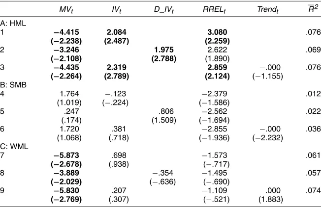
We present the OLS regression results in Table 7. As shown in panel A, both IV and MV are strong predictors of HML, with an adjustedR2of>7% (row 1). We find very similar results if we use D_IV in place of IV (row 2) or add a linear time trend to the forecasting equation (row 3). The coefficients on IV and MV have opposite signs to those reported in Table 2 for stock market returns, possibly because HML and stock market returns are negatively correlated.
MV is also a significant predictor for WML, as shown in panel C of Table 7, with an adjustedR2of around 6%. MV has a negative coefficient, possibly because WML and stock mar-ket returns are negatively correlated. We obtained the momen-tum profit from Ken French at Dartmouth College; Guo (2005) found the same results using the momentum data constructed by Jegadeesh and Titman (2001) and showed that innovations in MV explain a large portion of the observed momentum profit. In contrast, panel B of Table 7 shows that our forecasting variables have weak explanatory power for SMB. This latter result is not too surprising, however, given that the quarterly
average of SMB is an insignificant .45% in our sample pe-riod 1963:Q4–2002:Q4, compared with a significant 1.16% for HML and 2.75% for WML. Overall, our results again indi-cate that IV is a pervasive macrovariable because it captures systematic movements of HML, which has been interpreted as a hedging factor for time-varying investment opportunities (e.g., Campbell and Vuolteenaho 2004; Brennan, Wang, and Xia 2004).
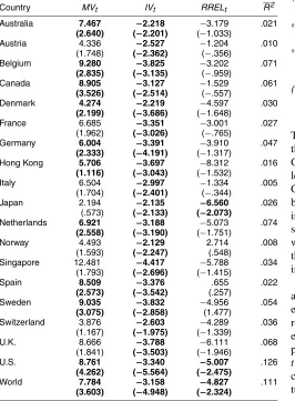
4.3 Forecasting Returns on International
Stock Market Indices
Given that the U.S. equity market is a large portion of the world equity market, IV should also forecast returns on inter-national stock market indices if it is a pervasive macrovariable. Table 8 presents the forecasting results using 18 international stock market indices and a measure of world stock market index, obtained from MSCI. The sample spans 1970:Q1– 2002:Q4. All the indices are denominated in U.S. dollars, and we use the U.S. risk-free rate to calculate the excess returns for each index. Interestingly, IV is statistically significant at the 5% level in all cases. Similarly, MV is significant at the 5% level in 11 cases and significant at the 10% level in 6 cases. However, RREL appears to be a weak forecasting variable for international stock market returns.
4.4 IV and Consumption–Wealth Ratio
Guo (2006) found a positive risk–return relation by control-ling for CAY in the forecasting equation of stock market re-turns. His results also suggest an omitted variables problem: Whereas CAY and MV are negatively related to each other, they are positively related to future stock market returns. Hence the behavior of CAY in the forecasting regression is similar to what we found for IV, suggesting that the two variables may be
re-Table 7. Forecasting Portfolio Returns, 1963:Q4–2002:Q4
MVt IVt D_IVt RRELt Trendt R2
A: HML
1 −4.415 2.084 3.080 .076
(−2.238) (2.487) (2.259)
2 −3.246 1.975 2.622 .069
(−2.108) (2.788) (1.890)
3 −4.435 2.319 2.859 −.000 .076
(−2.264) (2.789) (2.124) (−1.155)
B: SMB
4 1.764 −.123 −2.379 .012
(1.019) (−.224) (−1.586)
5 .247 .806 −2.562 .022
(.174) (1.509) (−1.694)
6 1.720 .381 −2.855 −.000 .036
(1.068) (.718) (−1.936) (−2.232) C: WML
7 −5.873 .698 −1.573 .061
(−2.678) (.938) (−.717)
8 −3.889 −.354 −1.495 .057
(−2.029) (−.636) (−.690)
9 −5.830 .207 −1.109 .000 .074
(−2.769) (.307) (−.521) (1.883)
NOTE: We report the OLS estimation results of the one-quarter-ahead portfolio returns on some predetermined variables. HML is the return on a portfolio that is long in stocks with high book-to-market value ratios and short in stocks with low book-to-market value ratios. SMB is the return on a portfolio that is long in small stocks and short in big stocks. WML is the return on a portfolio that is long in past winners and short in past losers. The heteroscadesticity-correctedtstatistics are in parentheses, and bold denotes significance at the 5% level.MVtis stock market volatility,IVtis idiosyncratic volatility,D_IVt is detrended idiosyncratic volatility,RRELtis the stochastically detrended risk-free rate, andTrendtis a linear time trend.
Table 8. Forecasting Quarterly Returns on International Stock Market Indices
Country MVt IVt RRELt R2
Australia 7.467 −2.218 −3.179 .021 (2.640) (−2.201) (−1.033)
Austria 4.336 −2.527 −1.204 .010 (1.748) (−2.362) (−.356)
Belgium 9.280 −3.825 −3.202 .071 (2.835) (−3.135) (−.959)
Canada 8.905 −3.127 −1.529 .061
(3.526) (−2.514) (−.557)
Denmark 4.274 −2.219 −4.597 .030 (2.199) (−3.686) (−1.648)
France 6.685 −3.351 −3.001 .027
(1.962) (−3.026) (−.765)
Germany 6.004 −3.391 −3.910 .047 (2.333) (−4.191) (−1.317)
Hong Kong 5.706 −3.697 −8.312 .016 (1.116) (−3.043) (−1.532)
Italy 6.504 −2.997 −1.334 .005
(1.704) (−2.401) (−.344)
Japan 2.194 −2.135 −6.560 .026
(.573) (−2.133) (−2.073)
Netherlands 6.921 −3.188 −5.073 .074 (2.558) (−3.190) (−1.751)
Norway 4.493 −2.129 2.714 .008
(1.593) (−2.247) (.548)
Singapore 12.481 −4.417 −5.788 .034 (1.793) (−2.696) (−1.415)
Spain 8.509 −3.376 .655 .022
(2.573) (−3.542) (.257)
Sweden 9.035 −3.832 −4.956 .054
(3.075) (−2.858) (1.477)
Switzerland 3.876 −2.603 −4.289 .036 (1.167) (−1.975) (−1.339)
U.K. 8.666 −3.788 −6.111 .068
(1.841) (−3.503) (−1.946)
U.S. 8.761 −3.340 −5.007 .126
(4.262) (−5.564) (−2.475)
World 7.784 −3.158 −4.827 .111
(3.603) (−4.948) (−2.324)
NOTE: We report the OLS estimation results of the one-quarter-ahead excess returns on the international stock market indices constructed by MSCI. The heteroscadesticity-corrected
tstatistics are in parentheses and bold denotes significance at the 5% level.MVtis stock market volatility,IVtis idiosyncratic volatility, andRRELtis the stochastically detrended risk-free rate. The sample spans 1970:Q1–2002:Q4.
lated. Indeed, as shown in Table 1, IV is strongly correlated with CAY, with a correlation coefficient of−.52.
Figure 4. Recursive MSE Ratio of Model With IV to Model Without IV (Table 9).
We formally investigate the relation between IV and CAY in Table 9. Row 1 confirms Lettau and Ludvigson’s (2001) results that CAY is a strong predictor of excess returns. Consistent with Guo (2006), whereas MV by itself is insignificant at the 5% level (row 2), it becomes highly significant if we also include CAY in the forecasting equation (row 3). Also note that CAY becomes more significant and the adjustedR2is much higher in row 3 than in rows 1 and 2. As mentioned earlier, these re-sults likely reflect an omitted variables problem. Furthermore, we find essentially the same results if we also include RREL in the forecasting equation (row 4). Therefore, CAY has forecast-ing patterns very similar to those of IV, as reported in Table 2.
To investigate whether forecasting abilities of CAY and IV are related, we include both CAY and IV in the forecasting equation; we report the results in row 5 of Table 9. Although IV remains significantly negative, the absolute values of its point estimate and t value are substantially smaller than those re-ported in row 5 of Table 2. Similarly, the point estimate and tvalue of CAY attenuate noticeably as well. These results indi-cate that IV and CAY share at least some information about fu-ture stock market returns. However, these results are potentially vulnerable to the criticism of spurious regression because of the deterministic trend in IV. Interestingly, IV becomes insignifi-cant at the 5% level if we add a linear time trend to the forecast-ing equation (row 7); D_IV is insignificant as well (row 6). In contrast, CAY is always significantly positive in rows 6 and 7. To further investigate this issue, Figure 4 plots the recursive MSE ratio of the model that uses CAY, VAR, RREL, and IV as forecasting variables to the model using only CAY, VAR, and
Table 9. Idiosyncratic Volatility and Consumption-Wealth Ratio
MVt IVt D_IVt RRELt Trendt CAYt R2
1 1.704 .066
(3.410)
2 2.907 .015
(1.681)
3 6.110 2.498 .139
(3.770) (5.067)
4 5.630 −3.760 2.354 .150
(3.528) (−1.737) (4.766)
5 10.077 −2.528 −4.129 1.806 .186
(4.429) (−3.326) (−1.995) (3.462)
6 7.156 −1.352 −3.746 1.907 .154
(3.432) (−1.121) (−1.760) (2.641)
7 10.075 −2.067 −4.263 −.000 2.051 .185
(4.449) (−1.938) (−2.102) (−.766) (2.898)
NOTE: We report the OLS regression results of the one-quarter-ahead excess stock market return on some predeter-mined variables. The heteroscadesticity-correctedtstatistics are in parentheses, and bold denotes significance at the 5% level.MVtis stock market volatility,IVtis idiosyncratic volatility,D_IVtis detrended idiosyncratic volatility,RRELtis the sto-chastically detrended risk-free rate,Trendtis a linear time trend, andCAYtis the consumption–wealth ratio. The sample spans 1963:Q4–2002:Q4.
RREL. Again, we find that IV provides little additional infor-mation beyond CAY. Therefore, IV forecasts stock market re-turns mainly because of its negative co-movements with CAY.
4.5 IV and Aggregate Stock Market Liquidity
In this section, we investigate whether IV is related to ag-gregate liquidity. As mentioned in Section 1, such a relation is consistent with existing theories. For example, Guo (2004) argued that CAY, which is closely related to IV (Table 9), is a proxy for the liquidity premium. Alternatively, various liquidity measures are closely related to the dispersion of opinion, which is negatively related to conditional excess stock returns of Cao et al. (2005).
Liquidity is a broad and elusive concept that generally de-notes the ability to trade large quantities at low cost without moving the price (see Pastor and Stambaugh 2003). In the em-pirical literature liquidity has been defined in many different ways, to capture various aspects of liquidity. To be robust, we investigate whether IV is related to various measures of aggre-gate liquidity analyzed by Chordia et al. (2001, 2002), which were generously provided to us by Avanidhar Subrahmanyam. One advantage of their measures is that many of them are con-structed using the intraday transaction data from the Institute for Study of Securities Markets (ISSM) and New York Stock Exchange TAQ (trades and automated quotations). However, the data span a relatively short sample period, 1988–2002, and our results should be interpreted with caution. The data were originally available on a daily basis, and we converted them into quarterly data using quarterly averages.
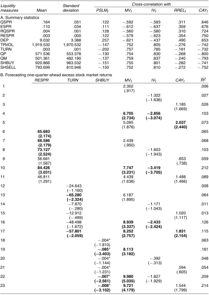
Panel A of Table 10 provides summary statistics of various liquidity measures constructed by Chordia et al. (2001, 2002). There are four measures of bid–ask spread, which are prox-ies for illiquidity: QSPR, the quoted spread; ESPR, the effec-tive spread; RQSPR, the relaeffec-tive quoted spread; and RESPR, the relative effective spread. There are seven measures of trad-ing activity, which are proxies for liquidity: DEP, depth, in thousands of shares; TRVOL, CRSP trading volume, in thou-sands of shares; TURN, CRSP turnover; QP, the number of buy trades; QM, the number of sell trades; SHBUY, shares bought in thousands; and SHSELL, shares sold in thousands. We find that these measures are only moderately correlated with Pastor and Stambaugh’s liquidity measure, PSLM; in contrast, they are highly correlated with IV, as well as with MV and CAY.
Panel B of Table 10 reports the regression results of fore-casting one-quarter-ahead excess stock market returns. We al-ways include a linear time trend (not reported in the table) in the regression because Chordia et al. (2001, 2002) showed that liquidity (illiquidity) has increased (decreased) over the past decade. To conserve space, we report only results using RESPR, TURN, and SHBUY. Nevertheless, as discussed later, we find similar results using the other measures (available on request). We also exclude RREL in the regression, because it is statis-tically insignificant in the recent sample period, as shown in Table 3. Of course, adding RREL to the forecasting equation has little effect on our results.
We first replicate our main findings over the short sample pe-riod 1988:Q2–2002:Q4. MV, IV, and CAY are insignificant in-dividually, as shown in rows 1–3. However, IV (row 4) and CAY
(row 5) become significant when combined with MV. Similarly, MV becomes significant in row 4 and marginally significant in row 5 when combined with IV and CAY, respectively.
Consistent with the findings of Jones (2002), we find that the bid–ask spread (RESPR) is positively and significantly re-lated to future excess stock market returns (row 6); however, it becomes insignificant after we control for CAY, with (row 11) and without (row 9) MV in the forecasting equation. Similarly, adding RESPR to the forecasting equation makes CAY insignif-icant in row 11. Therefore, our results indicate that RESPR and CAY share some similar information about future returns. How-ever, RESPR remains significant after we control for IV (rows 8 and 10). We also find qualitatively similar results using QSPR, ESPR, and RQSPR.
Jones (2002) also found that turnover (TURN) is negatively related to future stock market returns. We find that TURN is sta-tistically insignificant by itself (row 12); however, interestingly, it becomes significantly negative when combined with MV, and MV also becomes marginally significant (row 13). In contrast, TURN remains insignificant when combined with IV (row 14) and CAY (row 15). It is insignificant when combined with MV and IV (row 16). However, it is significant when combined with MV and CAY (row 17). Overall, these results indicate that the turnover has some forecasting abilities similar to those of IV and CAY.
SHBUY is negative and marginally significant by itself (row 18). Interestingly, similar to CAY or IV, it becomes highly significant after controlling for MV, and MV becomes highly significant as well (row 19). In contrast, it becomes insignifi-cant when combined with IV (row 20) and CAY (row 21), and IV and CAY are insignificant as well. It drives out IV (row 22) and CAY (row 23) from the forecasting equation when com-bined with MV. The latter result indicates that IV and CAY forecast returns mainly because they are proxies for the liquid-ity premium or the dispersion of opinion. However, this result should be interpreted with caution because of the small sample size. In particular, we find that SHBUY forecasts returns mainly because it is highly correlated with the trading volume, which is driven out by CAY in a longer sample from 1963 to 2002 (not reported). Similarly, we find essentially the same results using QP, QM, and SHSELL, which are all highly correlated with the trading volume. Moreover, the order imbalance—the difference between SHBUY and SHSELL—is strongly and positively cor-related with the trading volume; it is also a strong predictor of stock market returns when combined with MV. Moreover, we also find that the trading volume forecasts stock market returns when combined with stock market volatility in a longer sample from 1963 to 2002. DEP is not significantly related to future stock market returns, however. We also investigate Pastor and Stambaugh’s liquidity measure, PSLM and, interestingly, find that PSLM also forecasts stock market returns mainly because of its strong (negative) co-movements with MV; however, it is only moderately correlated with IV and CAY. Finally, we find that the liquidity measure proposed by Amihud (2002) does not forecast stock returns over our quarterly sample.
Overall, our results indicate that IV is closely related to some standard liquidity measures.
Table 10. Idiosyncratic Volatility and Aggregate Liquidity Measures
Liquidity measures
Standard deviation
Cross-correlation with
Mean PSLMt MVt IVt RRELt CAYt
A. Summary statistics
QSPR .164 .051 .122 −.592 −.583 .311 .646
ESPR .110 .034 .111 −.612 −.637 .359 .676
RQSPR .004 .001 .128 −.560 −.580 .310 .724
RESPR .003 .000 .122 −.579 −.623 .354 .750
DEP 9.032 3.388 .257 −.621 −.437 .490 .653
TRVOL 1,919.532 1,970.532 −.147 .752 .805 −.276 −.742
TURN .003 .001 −.202 .757 .785 −.181 −.732
QP 571.536 553.378 −.130 .754 .830 −.268 −.800
QM 501.361 482.190 −.137 .759 .837 −.240 −.793
SHBUY 920.866 963.532 −.151 .755 .801 −.282 −.741
SHSELL 793.699 810.946 −.150 .752 .810 −.272 −.752
B. Forecasting one-quarter-ahead excess stock market returns
RESPR TURN SHBUY MVt IVt CAYt R2
1 2.302 .006
(.917)
2 −1.322 .027
(−1.636)
3 1.185 .026
(1.669)
4 6.705 −2.856 .103
(2.734) (−3.074)
5 5.095 2.037 .073
(1.876) (2.440)
6 65.683 .065
(2.174)
7 66.586 2.439 .068
(2.179) (.950)
8 73.127 −1.603 .103
(2.524) (−1.943)
9 56.681 .653 .059
(1.587) (.738)
10 84.426 7.747 −3.419 .212
(3.031) (3.231) (−3.705)
11 46.811 4.439 1.488 .089
(1.291) (1.636) (1.466)
12 −24.643 .008
(−1.160)
13 −65.280 6.187 .064
(−2.324) (1.895)
14 −7.870 −1.171 .011
(−.280) (−1.043)
15 −12.912 1.020 .013
(−.489) (1.117)
16 −48.498 8.939 −2.433 .126
(−1.672) (3.337) (−2.424)
17 −57.801 8.252 1.831 .115
(−2.059) (2.757) (2.154)
18 −.004∗ .063
(−1.810)
19 −.085∗ 8.113 .181
(−3.403) (3.182)
20 −.004∗ −.392 .048
(−1.144) (−.313)
21 −.004∗ .594 .054
(−1.231) (.605)
22 −.007∗ 9.980 −1.827 .209
(−2.561) (5.035) (−1.929)
23 −.008∗ 9.721 1.544 .214
(−3.102) (4.179) (1.799)
NOTE: Panel A presents summary statistics. We report the OLS regression results of the one-quarter-ahead excess stock market return on some prede-termined variables in panel B. We also control for a linear time trend in the forecasting equation, which is not reported here. The heteroscadesticity-corrected
tstatistics are in parentheses, and bold denotes significance at the 5% level.PSLMtis Pastor and Stambaugh’s (2003) liquidity measure,MVtis realized stock market volatility,IVtis realized idiosyncratic volatility,RRELtis the stochastically detrended risk-free rate, andCAYtis the consumption-wealth ratio. The other liquidity measures are the same as those used by Chordia et al. (2001, 2002). There are four measures of bid–ask spread, which are proxies for
illiquidity: QSPR is quoted spread, ESPR is effective spread, RQSPR is relative quoted spread, and RESPR is relative effective spread. There are seven measures of trading activities, which are proxies for liquidity. DEP is depth in thousands of shares, TRVOL is CRSP trading volume in thousands of shares, TURN is CRSP turnover, QP is number of buy trades, QM is number of sell trades, SHBUY is shares bought in thousands, and SHSELL is shares sold in thousands. The sample spans 1988:Q2–2002:Q4.
∗Scaled by 100.
5. CONCLUSION
In this article, we find that the value-weighted idiosyncratic stock volatility is a strong predictor of excess stock market re-turns when combined with stock market volatility. Contrary to the nondiversification hypothesis, a high level of IV is usu-ally associated with low expected future stock returns. More-over, its forecasting abilities are very similar to those of the consumption–wealth ratio and some standard measures of ag-gregate stock market liquidity. Overall, our results indicate that IV is a pervasive macrovariable that captures systematic move-ments in stock returns; in particular, it might be a proxy for volatility of a risk factor of a multifactor or ICAPM model omit-ted from the CAPM.
Our results shed light on the out-of-sample stock return pre-dictability, for which recent authors (e.g., Bossaerts and Hillion 1999; Goyal and Welch 2003) found little support using con-ventional forecasting variables. The difference is explained by the fact that our forecasting variables drive out most variables used by the earlier authors, including dividend yield, term pre-mium, and default premium. We are also able to provide insight into the predictive power of CAY for stock returns, which has been questioned because it has a look-ahead bias and is subject to data revision. Our results suggest that the predictive power of CAY is not spurious, because IV—a variable available in real time—contains information about future stock returns that is very similar to that of CAY. Of course, IV should have more appeal than CAY to practitioners who must rely on real-time data to make portfolio choices.
The analysis in this article can be extended in several direc-tions. First, our results appear to be consistent with two alterna-tive explanations, that IV is a proxy for liquidity risk and that IV is a proxy for the dispersion of opinion. However, we do not distinguish between these two hypotheses, because liquid-ity and the dispersion of opinion are two closely related empir-ical concepts. We may use the underlying economic theories to develop more powerful tests to distinguish the two hypotheses in future research.
Second, our results indicate that along with a standard risk component, conditional excess stock market returns have an additional component, that is negatively related to the risk com-ponent. These results have an ICAPM interpretation, and it is interesting to investigate whether they can be related to the known CAPM-related anomalies. Also, recent work by Guo (2004) and Cao et al. (2005), among others, has provided ten-tative explanations for our results. However, the fundamental source of this additional risk factor remains unknown; for ex-ample, we do not know why the aggregate measure of stock market liquidity or the aggregate measure of the dispersion of opinion moves in a persistent manner, as documented in this ar-ticle. These issues warrant further investigation, both empirical and theoretical.
Third, the strong relation among IV, the consumption–wealth ratio, and aggregate liquidity reveals an important link between general equilibrium theories and market microstructure, as was recently emphasized by O’Hara (2003). These two approaches were explored separately in the early literature; however, a joint investigation should greatly improve our understanding of how asset prices are determined.
6. ACKNOWLEDGMENTS
The authors thank the editor, Torben G. Andersen, and an associate editor (the referee), whose many detailed and con-structive comments greatly improved the article. They are also grateful to Samuel Thompson, Tuomo Vuolteenaho, seminar participants at George Washington University and the Univer-sity of New Hampshire, and participants at the 2004 Missouri Economic Conference, the 2004 Financial Management As-sociation meeting, and the 2005 American Finance Associa-tion meeting for helpful suggesAssocia-tions. Martin Lettau, Kenneth French, and Avanidhar Subrahmanyam provided some of data used in this work. Jason Higbee provided excellent research as-sistance. The views expressed in this article are those of the authors and do not necessarily reflect the official positions of the Federal Reserve Bank of St. Louis or the Federal Reserve System.
[Received March 2004. Revised July 2005.]
REFERENCES
Acharya, V., and Pedersen, L. (2005), “Asset Pricing With Liquidity Risk,”
Journal of Financial Economics, forthcoming.
Amihud, Y. (2002), “Illiquidity and Stock Returns,”Journal of Financial Mar-kets, 5, 31–56.
Andersen, T., Bollerslev, T., Diebold, F., and Labys, P. (2003), “Modeling and Forecasting Realized Volatility,”Econometrica, 71, 579–625.
Ang, A., Hodrick, R., Xing, Y., and Zhang, X. (2005), “The Cross-Section of Volatility and Expected Returns,”Journal of Finance, forthcoming. Belsley, D., Kuh, E., and Welsch, R. (1980),Regression Diagnostics:
Identify-ing Influential Data and Sources of Collinearity, New York: Wiley. Bossaerts, P., and Hillion, P. (1999), “Implementing Statistical Criteria to
Se-lect Return Forecasting Models: What Do We Learn?”Review of Financial Studies, 12, 405–428.
Brennan, M., Wang, A., and Xia, Y. (2004), “Estimation and Test of a Simple Model of Intertemporal Asset Pricing,”Journal of Finance, 59, 1743–1775. Campbell, J. (1987), “Stock Returns and the Term Structure,”Journal of
Finan-cial Economics, 18, 373–399.
Campbell, J., Lettau, M., Malkiel, B., and Xu, Y. (2001), “Have Individual Stocks Become More Volatile? An Empirical Exploration of Idiosyncratic Risk,”Journal of Finance, 56, 1–43.
Campbell, J., Lo, A., and MacKinlay, C. (1997),The Econometrics of Financial Markets, Princeton, NJ: Princeton University Press.
Campbell, J., and Vuolteenaho, T. (2004), “Bad Beta, Good Beta,”American Economic Review, 94, 1249–1275.
Cao, H., Wang, T., and Zhang, H. (2005), “Model Uncertainty, Limited Market Participation and Asset Prices,”Review of Financial Studies, forthcoming. Chordia, T., Roll, R., and Subrahmanyam, A. (2000), “Commonality in
Liquid-ity,”Journal of Financial Economics, 56, 3–28.
(2001), “Market Liquidity and Trading Activities,”Journal of Finance, 56, 501–530.
(2002), “Order Imbalance, Liquidity and Market Returns,”Journal of Financial Economics, 65, 111–130.
Clark, T., and McCracken, M. (2001), “Tests of Equal Forecast Accuracy and Encompassing for Nested Models,”Journal of Econometrics, 105, 85–110. Diether, K., Malloy, C., and Scherbina, A. (2002), “Differences of Opinion and
the Cross-Section of Stock Returns,”Journal of Finance, 57, 2113–2141. Easley, D., Hvidkjaer, S., and O’Hara, M. (2002), “Is Information Risk a
De-terminant of Asset Returns?”Journal of Finance, 57, 2185–2221. Fama, E., and French, K. (1993), “Common Risk Factors in the Returns on
Stocks and Bonds,”Journal of Financial Economics, 33, 3–56.
(1996), “Multifactor Explanations of Asset Pricing Anomalies,” Jour-nal of Finance, 51, 55–84.
Ferson, W., Sarkissian, S., and Simin, T. (2003), “Spurious Regressions in Fi-nancial Economics?”Journal of Finance, 58, 1393–1414.
French, K., Schwert, W., and Stambaugh, R. (1987), “Expected Stock Returns and Volatility,”Journal of Financial Economics, 19, 3–29.
Ghysels, E., Santa-Clara, P., and Valkanov, R. (2005), “There Is a Risk-Return Trade-off After All,”Journal of Financial Economics, forthcoming.