Full Terms & Conditions of access and use can be found at
http://www.tandfonline.com/action/journalInformation?journalCode=ubes20
Download by: [Universitas Maritim Raja Ali Haji] Date: 12 January 2016, At: 00:26
Journal of Business & Economic Statistics
ISSN: 0735-0015 (Print) 1537-2707 (Online) Journal homepage: http://www.tandfonline.com/loi/ubes20
Decriminalization and Marijuana Smoking
Prevalence: Evidence From Australia
Kannika Damrongplasit, Cheng Hsiao & Xueyan Zhao
To cite this article: Kannika Damrongplasit, Cheng Hsiao & Xueyan Zhao (2010)
Decriminalization and Marijuana Smoking Prevalence: Evidence From Australia, Journal of Business & Economic Statistics, 28:3, 344-356, DOI: 10.1198/jbes.2009.06129
To link to this article: http://dx.doi.org/10.1198/jbes.2009.06129
Published online: 01 Jan 2012.
Submit your article to this journal
Article views: 877
Decriminalization and Marijuana Smoking
Prevalence: Evidence From Australia
Kannika D
AMRONGPLASITDepartment of Health Services, School of Public Health, University of California, Los Angeles, Los Angeles, CA 90095-1772; Rand Corporation, Santa Monica, CA 90407-2138, and Division of Economics, School of Humanities and Social Sciences, Nanyang Technological University, Singapore 637332
Cheng H
SIAODepartment of Economics, University of Southern California, Los Angeles, CA 90089; Department of Economics and Finance, City University of Hong Kong, Kowloon Tong, Kowloon, Hong Kong, and Wang Yanan Institute for Studies in Economics (WISE), Xiamen University, Xiamen, 361005 China (chsiao@usc.edu)
Xueyan Z
HAODepartment of Econometrics and Business Statistics, and Centre for Health Economics, Monash University, VIC 3800, Melbourne, Australia
This article uses the 2001 National Drug Strategy Household Survey to assess the impact of marijuana decriminalization policy on marijuana smoking prevalence in Australia. Both parametric and nonparamet-ric methods are used. The parametnonparamet-ric approach includes endogenous probit switching, two-part, sample selection, and standard dummy variable models, while the nonparametric approach uses propensity score stratification matching. Specification analyses are also conducted. A nonparametric kernel-based test is constructed to select between parametric and nonparametric models, and the likelihood ratio test is used to choose among parametric models. Our analyses favor the endogenous switching model where decrim-inalization increases the probability of smoking by 16.2%.
KEY WORDS: Average treatment effect; Bootstrapping; Endogenous probit switching; Illicit drugs; Parametric and nonparametric specification analysis; Propensity score matching.
1. INTRODUCTION
Illicit drug usage is widespread around the world, posing significant social and economic costs to the health care, jus-tice, and social welfare systems in both developed and devel-oping countries. According to the July 28, 2001 issue of the Economist, the global retail sale of illegal drugs is estimated at US$150 billion a year, which is in the same league as world-wide sale of tobacco and alcohol and about half the size of the pharmaceutical industry. Significant amounts of public funds have been spent by governments worldwide to deal with the consequences of substance abuse and on educational programs; for example, the United States’ drugs policy costs approxi-mately US$35–$40 billion a year according to the same issue of the Economist magazine, while the Australian government illicit drug expenditure has been estimated as AUD$3.2 billion for the year of 2002/3 (Moore2005).
Among illicit drugs, marijuana is by far the most widely used. It is commonly considered a “softer” drug compared with “harder” drugs, such as cocaine, heroin, or amphetamines. The prevalence of hydroponic cultivation in recent years has signif-icantly improved the productivity of covert production. While there is more support for using marijuana for medical purposes in treating patients with nausea, glaucoma, spasm, and pain, much controversy has surrounded the detrimental health ef-fects of recreational use of marijuana. Some suggest that mari-juana use is linked to lung cancer, immune system deterioration, harmful effects on blood circulation, and short-term memory
loss. For heavy users, there is also the problem of drug depen-dency and the related withdrawal symptoms, such as anxiety and loss of appetite.
At the center of the controversy is whether legal sanctioning is the best approach to reduce the use and the associated harm of the drug. The ongoing debate on marijuana decriminalization concentrates on the potential benefits and costs of such a pol-icy. A major supporting argument for decriminalization is that a criminal charge is too severe a penalty relative to the crime itself. A criminal record can have many negative consequences on the subsequent life of an otherwise law-abiding person; for example, an offender may lose out in future employment oppor-tunities or face problems in international travel. Furthermore, decriminalization would allow the government to separate the market of marijuana from the market of other, harder drugs, thereby permitting the authorities to redirect their resources used in law enforcement and criminal justice system from the “softer” cannabis to “harder” drugs like cocaine, heroin, and amphetamines. For instance, a 2005 report by Jeffrey Miron, “The Budgetary Implications of Marijuana Prohibition,” noted that legalizing marijuana could reduce the cost of enforcement in the United States by US$7.7 billion per year. Moreover, sup-porters also argue that when marijuana is illegal, young mari-juana users are unnecessarily exposed to harder drug dealers,
© 2010American Statistical Association
Journal of Business & Economic Statistics July 2010, Vol. 28, No. 3 DOI:10.1198/jbes.2009.06129
344
Damrongplasit, Hsiao, and Zhao: Decriminalization and Marijuana Smoking Prevalence 345
making it easier for them to move on to consume harder drugs. For those who argue against decriminalization, their first claim is that decriminalization inevitably lowers both the legal and social costs associated with the use of marijuana, thus send-ing a signal that it is acceptable to smoke marijuana, which may encourage higher consumption of the drug. Another ar-gument cited against decriminalization is the gateway theory; that is, there is a growing concern that exposure to marijuana by youths may lead to their subsequent consumption of other, harder drugs. Given the foregoing debates, empirical evidence of the impact of marijuana decriminalization on marijuana us-age is crucial. In particular, if decriminalization has little or no impact on smoking prevalence, then this is a strong argument in favor of the policy. On the other hand, if there is evidence that decriminalization significantly stimulates more marijuana smoking, then a liberal approach toward marijuana may not be as beneficial as is advocated by its supporters.
Empirical results using various data sources from the United States are mixed. Saffer and Chaloupka (1995,1998), and Pac-ula, Chriqui, and King (2003) found the impact of decriminal-ization on marijuana smoking prevalence to be positive and significant. In contrast, DiNardo and Lemieux (2001), Pacula (1998), and Thies and Register (1993) reported insignificant ef-fects of marijuana policy reform on individual smoking deci-sions. There have been three empirical studies of the Australian experience. Cameron and Williams (2001) and Zhao and Har-ris (2004) both found a positive and significant marginal effect of decriminalization on prevalence of about 2%, while Williams (2004) found it to be significant only for the subsample of males age 25 years old and older. Typically, binary probit models have been used in these studies, with the decriminalization dummy variable treated as an exogenous explanatory variable.
In this work, we used the 2001 Australian National Drug Strategy Household Surveys (NDSHS2001) to study the impact of marijuana decriminalization on marijuana usage. Australia consists of six states and two territories. As of 2001, South Aus-tralia, Australia Capital Territory, and Northern Territory had already decriminalized the possession and cultivation of small quantities of marijuana for personal consumption. Under this regulation, while supplying and cultivating commercial quan-tities of marijuana still attract severe criminal charges, an “on the spot” fine has replaced criminal charges for minor users. An individual caught using or growing marijuana must pay a fine (usually AUS$150–$200) within a specified period, usually within 60 days, to be eligible for the reduced penalty involving no criminal record or imprisonment. If the person fails to pay the fine, however, a criminal proceeding may follow, possibly leading to a jail sentence. The Australian policy of decriminal-ization is commonly known as the Cannabis Expiation Notice system (CEN). Finally, for those states that have not decrim-inalized marijuana, criminal offenses for possessing, consum-ing, and cultivating the drug are retained.
The present study aimed to assess the impact of decriminal-ization on marijuana smoking prevalence. There are three major differences between this study and earlier studies. First, existing studies usually treat decriminalization as an exogenous dummy variable when performing regression analysis. This is also the case here, because our data are based on the 2001 survey. As of 2001, three states in Australia had already decriminalized mar-ijuana use: South Australia in 1987, Australia Capital Territory
in 1992, and Northern Territory in 1996. Thus, in analyzing this set of data, we take a state’s decriminalization decision as pre-determined and focus on another source of joint dependence: marijuana smoking behavior and residential choice. At the in-dividual level, the decision of living in a particular state may not be random, and the decisions of where to live and whether to smoke may be related. Individuals may not be randomly se-lected to different states, and there may be selection bias arising from those living in the decriminalized states versus those in the nondecriminalized states. In this article we attempt to address the potential endogeneity of marijuana smoking and the indi-vidual’s decision to reside in a decriminalized versus a nonde-criminalized state by allowing an individual’s marijuana smok-ing behavior equation to be correlated with his or her residential choice. Second, we provide a more flexible marijuana smok-ing behavior equation by allowsmok-ing individuals to respond dif-ferently when the legal and institutional arrangement changes. Third, both parametric and nonparametric analyses are con-ducted, and their reliabilities are examined.
Essentially, the advantages of the parametric approach are the disadvantages of the nonparametric approach, and the ad-vantages of the nonparametric approach are the disadad-vantages of the parametric approach. The advantages of the parametric approach are that it can simultaneously take into account selec-tion on observables and unobservables (provided that the model is correctly specified) and allows (efficient) estimation of the ef-fects of individual factors on the outcomes. The disadvantages of the parametric approach are that both the conditional mean functions of observable factors and the probability distributions of the effects of unobservable factors must be specified. The advantages of the nonparametric approach are that neither the conditional mean functions of observable factors nor the proba-bility distributions of the effects of unobservable factors need to be specified. The disadvantages (of propensity score matching) are that it only takes into account selection on observables and only estimates the treatment effects. We discuss the pros and cons through our specification analyses.
The article is organized as follows. Section2presents an en-dogenous probit switching model as the maintained hypothe-sis and treat the traditional dummy variable approach, sample selection model, and two-part model as its nested alternatives, called the binary probit, bivariate probit, and two-part models, respectively. Section3provides a description of our data. Sec-tion4reports our estimation results and compares them with re-sults in the literature. Section5presents alternative measures of treatment effect from the propensity score stratification match-ing method. Section6presents specification analyses, and Sec-tion7concludes.
2. THE MODEL
We assume that the utility for an individual’s residential choice (d=1 if residing in decriminalized state and 0 if not) and marijuana consumption (M) is separable from the utility of consuming other goods. Similar to Carneiro, Hansen, and Heckman (2003), Keane and Wolpin (1997), and others, we assume that an individual’s utility function for marijuana con-sumption and residential choice is state-dependent on the initial endowment and institutional arrangement of the two residential
346 Journal of Business & Economic Statistics, July 2010
regimes. In particular, we let an individual’s utility function be U(M,d|a,a∗)=dU1(M|a)+(1−d)U0(M|a)+h(d|a∗), where U1(·) andU0(·)are the utility functions of consuming mari-juana for an individual residing in a decriminalized state and a nondecriminalized state, respectively;h(·)denotes the utility of living in decriminalized state or nondecriminalized state; anda and a∗ are sociodemographic, institutional, and idiosyncratic components that affect M andd, respectively. a and a∗ may contain overlapping elements.U1(·)andU0(·)are assumed to be different, because the same amount of marijuana consump-tion may lead to different levels of utility in decriminalized and nondecriminalized states because of differing institutional se-tups; for example, the risk of smoking marijuana could be dif-ferent.
Maximizing utility subject to budget constraint I yields M1(p,I|a)≥0 for an individual residing in a decriminalized state andM0(p,I|a)≥0 for an individual residing in a nonde-criminalized state, wherepdenotes price of marijuana. Substi-tutingM1(·)andM0(·)into the utility function yields the
condi-wherexdenotes the observable factors ofp,I, andathat affect the demand for marijuana andε1andε0denote the effects of unobservables. Equations (2.1)–(2.4) imply Prob(M1(x)=0)= note the additional observable factors ina∗that are not inaand the effects of unobservable factors in bothaanda∗that affect residential choice.
Our data are in the form(y,d), wherey=1 indicates that an individual is a marijuana smoker and 0 otherwise, andd=1 if an individual resides in a decriminalized state and 0 otherwise. From (2.1)–(2.4), it follows that
y=1 ifdy∗1+(1−d)y∗0>0 and
(2.6) y=0 otherwise.
Equations (2.1)–(2.6) lead to an endogenous switching model. The model is in a limited information framework in which we
have a structural form specification for the demand for mari-juana for individuals residing in a decriminalized state and a nondecriminalized state and a reduced-form specification for the residential choice. The identification of the structural mar-ijuana use equation is achieved through the excluded vari-ables,z, that are important in predicting the residential choice (e.g., Hsiao1983).
Many of the conventional models have become special cases of this model. For instance, we could have the following:
(a) Whenρ1υ=ρ0υ=0, it is known as a restricted
switch-ing model, where ρ1υ and ρ0υ denote the correlations
betweenε1andυand betweenε0andυ, respectively. (b) Whenρ1υ =ρ0υ=0, the residential choice equation’s
error term is uncorrelated with the smoking equations. In this case, model (2.1)–(2.6) is a generalization to the frequently used two-part model (Duan et al.1983,1984) or the exogenous regime-switching model of Quandt (1972).
(c) When β1 =β0 =β, and ρ1υ =ρ0υ =0, the model
is analogous to the sample selection model (Amemiya 1985) in which duces to dummy variable approach to evaluating the ef-fect of decriminalization withM given by (2.7) and un-correlated with (2.5).
Therefore, we may estimate the average treatment effect (ATE) by
[ (α1+β1x)− (α0+β0x)]f(x)dx (2.8) and the average treatment effect of the treated (ATET) by
[ (α1+β1x)− (α0+β0x)]f(x|d=1)dx (2.9) or their restricted version, where (a)denotes the integrated standard normal from −∞ to a. If the sample is randomly drawn, then the ATE or ATET may be approximated by
1
where the summation is over the complete sample or over those residing in a decriminalized state.
In what follows, we first present parametric analysis, then nonparametric analysis. We show that the results are sensitive to model specifications and discuss which model is likely to yield more accurate measurements of the effects of decriminal-ization.
Damrongplasit, Hsiao, and Zhao: Decriminalization and Marijuana Smoking Prevalence 347
3. DESCRIPTION OF VARIABLES AND DATA
3.1 Selection of Explanatory Variables
Marijuana is an addictive recreational drug, and studies on recreational drugs have arisen from many disciplines, such as psychology, medicine, epidemiology, sociology, and eco-nomics. Maximizing the state-dependent utility function leads to demand for marijuana as a function of price, income, as well as some standard socioeconomic and demographic vari-ables that capture heterogeneity in demand, such as age, sex, marital status, educational attainment, work status, and ethnic background for the Australian indigenous population, as com-monly postulated in empirical studies (e.g., Becker and Murphy 1988; Pacula1998; Williams2004; Zhao and Harris2004). The impact of the legal risk of smoking via the decriminalization policy is captured by allowing the responses to the conditional variables to be different for the two types of states using the endogenous switching model described earlier.
For residential choice, the literature (Feridhanusetyawan and Kilkenny 1996; Kittiprapas and McCann1999) suggests that both personal and location characteristics are key determinants of an individual’s residential choice. Because we are taking a limited-information approach, in addition to those variables de-termining marijuana smoking, additional variables, including number of dependent children (which might influence residen-tial choice) and unemployment rate in each individual’s state of residence (a proxy for state-specific effects) are also used to predict residential choice as well as to provide exclusion restric-tions needed to identify the marijuana use behavioral equarestric-tions (see, e.g., Hsiao1983).
3.2 Data
The data used come from three different sources: the 2001 Australia National Drug Strategy Household Survey (NDSHS
2001), the Australia Bureau of Statistics (ABS), and the Aus-tralian Illicit Drug Report. The NDSHS is a nationally repre-sentative household survey of the noninstitutionalized civilian Australian population age 14 and older. It provides information on individual drug use, as well as many socioeconomic and de-mographic variables. Three different survey methods were im-plemented: a drop-and-collect questionnaire, a face-to-face per-sonal interview, and a computer-assisted telephone interview. For more sensitive questions (e.g., individual drug use), mea-sures were put in place to keep the information confidential from the interviewer, in order to minimize potential underre-porting of drug use. A total of 26,744 observations were avail-able in the 2001 wave of NDSHS. In addition, the 2001 NDSHS also provides information on explanatory variables, including household income (Income), age (Age1419,Age2024,Age2529, Age3034,Age3539,Age4069,Age70), sex (Male), marital sta-tus (Married,Divorce,Widow,Never married), number of de-pendent children (#depchild), educational attainment (Degree), employment status (Working status), and ethnicity ( Aborigi-nal). A dichotomous variable (Decrim) is also defined, indicat-ing whether a person resides in a decriminalized state. After ob-servations with missing data were deleted, the resulting sample comprised 14,008 observations. Because South Australia, Aus-tralia Capital Territory, and Northern Territory had already de-criminalized marijuana by 2001, observations from these three states were classified as the treatment group. Table1defines all variables.
The price of marijuana was obtained from the Australia Bu-reau of Criminal Intelligence (ABCI2002) and the Australian Crime Commissions (ACC2003). Four different prices by state were available: price of head per ounce, price of head per gram, price of leaf per ounce, and price of leaf per gram. These prices were first converted to the same unit, price per ounce. Then
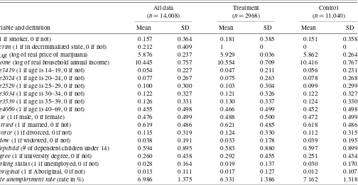
Table 1. Summary statistics of dependent and independent variables (n=14,008)
All data Treatment Control (n=14,008) (n=2968) (n=11,040)
Variable and definition Mean SD Mean SD Mean SD
y(1 if smoker, 0 if not) 0.157 0.364 0.181 0.385 0.151 0.358
Decrim(1 if in decriminalized state, 0 if not) 0.212 0.409 1 0 0 0
PMAR(log of real price of marijuana) 5.876 0.237 5.929 0.036 5.862 0.264
Income(log of real household annual income) 10.445 0.757 10.554 0.709 10.416 0.767
Age1419(1 if age is 14–19, 0 if not) 0.054 0.227 0.047 0.211 0.056 0.231
Age2024(1 if age is 20–24, 0 if not) 0.077 0.267 0.075 0.263 0.078 0.268
Age2529(1 if age is 25–29, 0 if not) 0.100 0.300 0.103 0.304 0.099 0.299
Age3034(1 if age is 30–34, 0 if not) 0.122 0.327 0.121 0.326 0.122 0.327
Age3539(1 if age is 35–39, 0 if not) 0.126 0.331 0.130 0.337 0.124 0.330
Age4069(1 if age is 40–69, 0 if not) 0.455 0.498 0.466 0.499 0.452 0.498
Male(1 if male, 0 if female) 0.476 0.499 0.488 0.500 0.472 0.499
Married(1 if married, 0 if not) 0.619 0.486 0.621 0.485 0.618 0.486
Divorce(1 if divorced, 0 if not) 0.115 0.319 0.124 0.330 0.112 0.315
Widow(1 if widowed, 0 if not) 0.038 0.191 0.033 0.178 0.039 0.195
# depchild(# of dependent children under 14) 0.594 0.895 0.583 0.880 0.597 0.899
Degree(1 if university degree, 0 if not) 0.260 0.438 0.292 0.455 0.251 0.434
Working status(1 if unemployed, 0 if not) 0.028 0.164 0.019 0.137 0.030 0.170
Aboriginal(1 if Aboriginal, 0 if not) 0.013 0.111 0.017 0.127 0.012 0.107
State unemployment rate(rate in %) 6.986 1.375 6.331 1.386 7.162 1.318
348 Journal of Business & Economic Statistics, July 2010
for each state, a weighted average of the four prices was com-puted using proportions of the respondents’ form of purchase as weights. Each state’s weighted average price of marijuana was deflated by the state’s CPI, and a logarithmic function was applied. The final price of marijuana is denoted byPMAR. A thorough discussion of Australia’s marijuana price has been provided by Clements (2004). State-level CPIs and state-level unemployment rates are drawn from the Australia Bureau of Statistics (ABS2003a,2003b), with the latter expressed as per-centages. Table1provides summary statistics of dependent and independent variables for all observations, treatment observa-tions, and control observations.
4. EMPIRICAL RESULTS
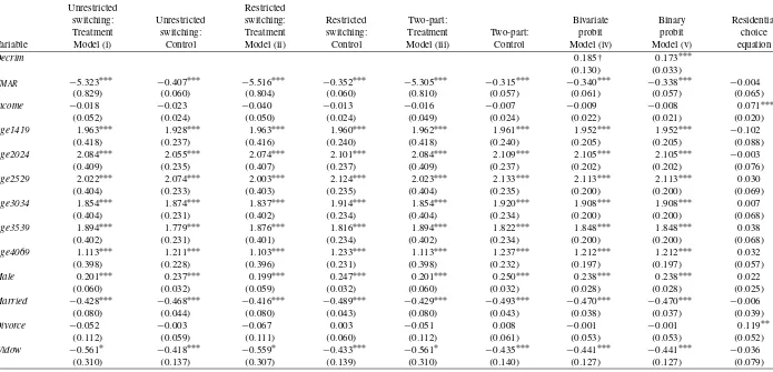
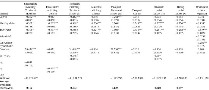
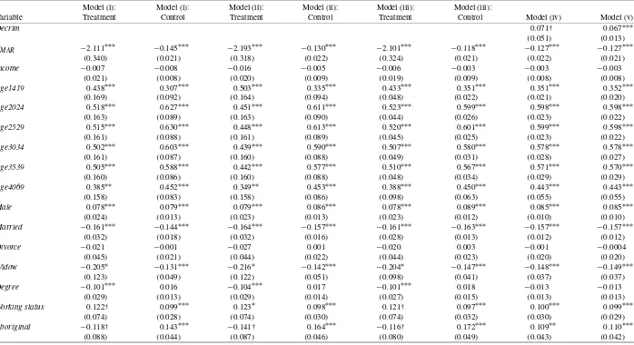
We used the maximum likelihood method to derive our pa-rameter estimates. Because we do not simultaneously observe y∗1 andy∗0, the joint distribution of (ε1, ε0) orρ10 is not iden-tified. Table2 reports estimated coefficients for the marijuana use and the reduced-form residential choice equations and the average treatment effects for all five models studied. Table 3 provides estimates of the marginal effects on marijuana partic-ipation probability for a reference individual, a male age 14– 19 years with less than a university education, never married, not unemployed, not of Aboriginal origin, residing in a nonde-criminalized state, having income equal to the mean of house-hold income, and facing marijuana price equal to the mean price.
Our results show that decriminalization has positive and gen-erally significant impacts on marijuana smoking behavior, al-though the magnitude of these effects varies across different models. The ATE of decriminalization for all models is given at the bottom of Table2and the marginal effects of specific factors for our reference individual are specified in Table3. We first discuss each model’s estimated ATE. When using a simple bi-nary probit model not accounting for endogeneity of treatment and flexibility in behavior, the estimated ATE is 3.7%. This is very similar to the values estimated by Cameron and Williams (2001) and Zhao and Harris (2004). When accounting for en-dogeneity of treatment as in model (iv), the ATE rises to 4%. However, when allowing for behavioral differences between the treatment and the control groups but ignoring endogenous treat-ment as in the two-part model, the ATE is 13.7%. Finally, in the endogenous probit switching models (i) and (ii), the estimated ATEs are 16.2% and 18.3%, respectively. It is clear that the two-part and the endogenous probit switching models provide stronger support to the opponents of marijuana decriminaliza-tion policy, because they yield substantially larger ATEs than the binary probit and the bivariate probit models.
For the impact of specific explanatory variables on mari-juana use behavior, models (i), (ii), and (iii) yield similar re-sults, while models (iv) and (v) generate comparable outcomes. Consistent with an a priori conjecture that demand is nega-tively associated with the price of marijuana, the coefficients of PMAR are negative and significant for all models, implying a negative own-price responsiveness. For a reference person, a 10% increase in the price of marijuana decreases the probabil-ity of using it by 1.27% according to our binary probit and the
bivariate probit models. When allowing for behavioral differ-ences between the treatment and control groups and/or taking into account possible endogeneity, we find a much larger nega-tive own-price effect in the decriminalized states. In particular, for a reference person, as marijuana price increases by 10%, the probability of using the drug is estimated to fall by approxi-mately 21% in decriminalized states, but by only 1.18%–1.45% in nondecriminalized states. The higher price responsiveness in the decriminalized states is expected, because we would ex-pect price to play a much smaller role in the nondecriminalized states where the risk premium of being caught should have a greater role than price in the smoking decision.
If marijuana were a normal good, then we would expect the coefficient of household income to be positive and significant. But the coefficient of household income is negative but insignif-icant for all models studied. This indicates an absence of in-come effect. The literature reports mixed results on inin-come. For example, a full-sample estimation by Saffer and Chaloupka (1998) found an insignificant effect of income on the probabil-ity of marijuana use, while Pacula (1998) and Thies and Regis-ter (1993) both reported a significant negative income effect.
As for other conditional variables that affect marijuana use behavior, age is an important factor affecting marijuana smok-ing behavior. Cameron and Williams (2001) and Williams (2004) both reported that the probability of participating in mar-ijuana peaks at age 20–24 years and then declines monoton-ically thereafter. Our maximum likelihood coefficients in Ta-ble2obtain this same finding for the treatment group of mod-els (i), (ii) and (iii); however, for the other modmod-els [i.e., the control group of models (i), (ii), and (iii), model (iv), and model (v)], smoking prevalence peaks at age 25–29. Our results indicate that young adults have the highest risk of becoming marijuana smokers in decriminalized states, while adults have the greatest exposure in nondecriminalized states.
We find a positive and significant coefficient on the gen-der dummy variable across models, in agreement with previ-ous studies. Married individuals are less likely to use marijuana than their never-married counterparts. Widowed individuals are less likely to be marijuana smokers for all models and for both the treatment and control groups. No difference in smoking be-havior was noted between divorced and single persons across all models.
Education attainment does not seem to play a role in the deci-sion to consume marijuana when using models (iv) and (v). But when allowing for behavioral differences due to policy changes, as in model (iii), and possible endogeneity of treatment, as in models (i) and (ii), the effects of education differ across the treatment and control groups. For those who live in decriminal-ized states, having a university degree substantially reduces the likelihood of smoking marijuana. In contrast, for those living in nondecriminalized states, marijuana smoking prevalence is similar in those with and without tertiary education.
In this study,Working statusis assigned a value of 1 if the individual is unemployed and 0 otherwise. The coefficient of Working statusis found to be positive and significant for bi-nary probit, bivariate probit, the control group of two-part, re-stricted, and unrestricted endogenous probit switching models. The estimated marginal effect in Table3suggests that a refer-ence individual can have up to 12% greater chance of becoming
Damrongplasit,
H
siao
,
and
Zhao:
Decr
iminalization
and
Mar
ijuana
Smoking
P
re
valence
349
Table 2. Coefficient estimates for marijuana smoking and residential choice equations
Unrestricted Restricted
switching: Unrestricted switching: Restricted Two-part: Bivariate Binary Residential Treatment switching: Treatment switching: Treatment Two-part: probit probit choice Variable Model (i) Control Model (ii) Control Model (iii) Control Model (iv) Model (v) equation
Decrim 0.185† 0.173∗∗∗
(0.130) (0.033)
PMAR −5.323∗∗∗ −0.407∗∗∗ −5.516∗∗∗ −0.352∗∗∗ −5.305∗∗∗ −0.315∗∗∗ −0.340∗∗∗ −0.338∗∗∗ −0.004 (0.829) (0.060) (0.804) (0.060) (0.810) (0.057) (0.061) (0.057) (0.065)
Income −0.018 −0.023 −0.040 −0.013 −0.016 −0.007 −0.009 −0.008 0.071∗∗∗
(0.052) (0.024) (0.050) (0.024) (0.049) (0.024) (0.022) (0.021) (0.020)
Age1419 1.963∗∗∗ 1.928∗∗∗ 1.963∗∗∗ 1.960∗∗∗ 1.962∗∗∗ 1.961∗∗∗ 1.952∗∗∗ 1.952∗∗∗ −0.102
(0.418) (0.237) (0.416) (0.240) (0.418) (0.240) (0.205) (0.205) (0.088)
Age2024 2.084∗∗∗ 2.055∗∗∗ 2.074∗∗∗ 2.101∗∗∗ 2.084∗∗∗ 2.109∗∗∗ 2.105∗∗∗ 2.105∗∗∗ −0.003
(0.409) (0.235) (0.407) (0.237) (0.409) (0.237) (0.202) (0.202) (0.076)
Age2529 2.022∗∗∗ 2.074∗∗∗ 2.003∗∗∗ 2.124∗∗∗ 2.023∗∗∗ 2.133∗∗∗ 2.113∗∗∗ 2.113∗∗∗ 0.030
(0.404) (0.233) (0.403) (0.235) (0.404) (0.235) (0.200) (0.200) (0.069)
Age3034 1.854∗∗∗ 1.874∗∗∗ 1.837∗∗∗ 1.914∗∗∗ 1.854∗∗∗ 1.920∗∗∗ 1.908∗∗∗ 1.908∗∗∗ 0.007
(0.404) (0.231) (0.402) (0.234) (0.404) (0.234) (0.200) (0.200) (0.068)
Age3539 1.894∗∗∗ 1.779∗∗∗ 1.876∗∗∗ 1.816∗∗∗ 1.894∗∗∗ 1.822∗∗∗ 1.848∗∗∗ 1.848∗∗∗ 0.038
(0.402) (0.231) (0.401) (0.234) (0.402) (0.234) (0.200) (0.200) (0.068)
Age4069 1.113∗∗∗ 1.211∗∗∗ 1.103∗∗∗ 1.233∗∗∗ 1.113∗∗∗ 1.237∗∗∗ 1.212∗∗∗ 1.212∗∗∗ 0.032
(0.398) (0.228) (0.396) (0.231) (0.398) (0.232) (0.197) (0.197) (0.057)
Male 0.201∗∗∗ 0.237∗∗∗ 0.199∗∗∗ 0.247∗∗∗ 0.201∗∗∗ 0.250∗∗∗ 0.238∗∗∗ 0.238∗∗∗ 0.022
(0.060) (0.032) (0.059) (0.032) (0.060) (0.032) (0.028) (0.028) (0.025) Married −0.428∗∗∗ −0.468∗∗∗ −0.416∗∗∗ −0.489∗∗∗ −0.429∗∗∗ −0.493∗∗∗ −0.470∗∗∗ −0.470∗∗∗ −0.006
(0.080) (0.044) (0.080) (0.043) (0.080) (0.043) (0.038) (0.037) (0.039)
Divorce −0.052 −0.003 −0.067 0.003 −0.051 0.008 −0.001 −0.001 0.119∗∗
(0.112) (0.059) (0.111) (0.060) (0.112) (0.061) (0.053) (0.053) (0.052) Widow −0.561∗ −0.418∗∗∗ −0.559∗ −0.433∗∗∗ −0.561∗ −0.435∗∗∗ −0.441∗∗∗ −0.441∗∗∗ −0.036
(0.310) (0.137) (0.307) (0.139) (0.310) (0.140) (0.127) (0.127) (0.079)
350
Jour
nal
of
Business
&
Economic
Statistics
,
July
2010
Table 2. (Continued)
Unrestricted Restricted
switching: Unrestricted switching: Restricted Two-part: Bivariate Binary Residential Treatment switching: Treatment switching: Treatment Two-part: probit probit choice Variable Model (i) Control Model (ii) Control Model (iii) Control Model (iv) Model (v) equation
Degree −0.262∗∗∗ 0.043 −0.262∗∗∗ 0.046 −0.262∗∗∗ 0.047 −0.034 −0.034 −0.018
(0.073) (0.038) (0.073) (0.038) (0.073) (0.039) (0.034) (0.034) (0.030)
Working status 0.307† 0.265∗∗∗ 0.318∗ 0.256∗∗∗ 0.306† 0.249∗∗∗ 0.257∗∗∗ 0.256∗∗∗ −0.155∗
(0.188) (0.080) (0.186) (0.081) (0.187) (0.081) (0.075) (0.074) (0.083)
Aboriginal −0.308† 0.377∗∗∗ −0.356† 0.421∗∗∗ −0.304† 0.438∗∗∗ 0.281∗∗∗ 0.282∗∗∗ 0.319∗∗∗
(0.222) (0.123) (0.219) (0.124) (0.218) (0.124) (0.107) (0.107) (0.107)
# depchild −0.023†
(0.016)
State unemp- −0.286∗∗∗
loyment rate (0.012)
Constant 29.474∗∗∗ −0.021 31.049∗∗∗ −0.414 29.338∗∗∗ −0.650 −0.454 −0.468 0.408
(5.021) (0.478) (4.836) (0.471) (4.832) (0.457) (0.455) (0.429) (0.482)
ρ1υ=ρ0υ −0.148∗ −0.007
(0.083) (0.077)
ρ1υ −0.011
(0.109)
ρ0υ −0.465∗∗∗
(0.179)
Log
likelihood −11,928.667 −11,931.323 −1183.790 −3,997.998 −11,969.153 −5,218.030 −6,751.128
Average treatment
effect (ATE) 0.162 0.183 0.137 0.040 0.037
NOTE: (1) Standard errors are in parentheses, (2) *** significant at 1% (two-tailed test), (3) ** significant at 5% (two-tailed test), (4) * significant at 10% (two-tailed test), (5) † significant at 10% (one-tailed test), (6) The percentage of correct predictions for residential choice equation is found to be 78.87%, (7) notes (1)–(5) also apply to Table3.
Damrongplasit,
H
siao
,
and
Zhao:
Decr
iminalization
and
Mar
ijuana
Smoking
P
re
valence
351
Table 3. Marginal effects for marijuana smoking equation
Model (i): Model (i): Model (ii): Model (ii): Model (iii): Model (iii):
Variable Treatment Control Treatment Control Treatment Control Model (iv) Model (v)
Decrim 0.071† 0.067∗∗∗
(0.051) (0.013)
PMAR −2.111∗∗∗ −0.145∗∗∗ −2.193∗∗∗ −0.130∗∗∗ −2.101∗∗∗ −0.118∗∗∗ −0.127∗∗∗ −0.127∗∗∗
(0.340) (0.021) (0.318) (0.022) (0.324) (0.021) (0.022) (0.021)
Income −0.007 −0.008 −0.016 −0.005 −0.006 −0.003 −0.003 −0.003
(0.021) (0.008) (0.020) (0.009) (0.019) (0.009) (0.008) (0.008)
Age1419 0.438∗∗∗ 0.307∗∗∗ 0.503∗∗∗ 0.335∗∗∗ 0.433∗∗∗ 0.351∗∗∗ 0.351∗∗∗ 0.352∗∗∗
(0.169) (0.092) (0.164) (0.094) (0.048) (0.022) (0.021) (0.020)
Age2024 0.518∗∗∗ 0.627∗∗∗ 0.451∗∗∗ 0.611∗∗∗ 0.523∗∗∗ 0.599∗∗∗ 0.598∗∗∗ 0.598∗∗∗
(0.163) (0.089) (0.163) (0.090) (0.044) (0.026) (0.023) (0.022)
Age2529 0.515∗∗∗ 0.630∗∗∗ 0.448∗∗∗ 0.613∗∗∗ 0.520∗∗∗ 0.601∗∗∗ 0.599∗∗∗ 0.598∗∗∗
(0.161) (0.088) (0.161) (0.089) (0.045) (0.025) (0.023) (0.022)
Age3034 0.502∗∗∗ 0.603∗∗∗ 0.439∗∗∗ 0.590∗∗∗ 0.507∗∗∗ 0.580∗∗∗ 0.578∗∗∗ 0.578∗∗∗
(0.161) (0.087) (0.160) (0.088) (0.049) (0.031) (0.028) (0.027)
Age3539 0.505∗∗∗ 0.588∗∗∗ 0.442∗∗∗ 0.577∗∗∗ 0.510∗∗∗ 0.567∗∗∗ 0.571∗∗∗ 0.570∗∗∗
(0.160) (0.086) (0.160) (0.088) (0.048) (0.034) (0.029) (0.029)
Age4069 0.385∗∗ 0.452∗∗∗ 0.349∗∗ 0.453∗∗∗ 0.388∗∗∗ 0.450∗∗∗ 0.443∗∗∗ 0.443∗∗∗
(0.158) (0.083) (0.158) (0.086) (0.098) (0.063) (0.055) (0.055)
Male 0.078∗∗∗ 0.079∗∗∗ 0.079∗∗∗ 0.086∗∗∗ 0.078∗∗∗ 0.089∗∗∗ 0.085∗∗∗ 0.085∗∗∗
(0.024) (0.013) (0.023) (0.013) (0.023) (0.012) (0.010) (0.010)
Married −0.161∗∗∗ −0.144∗∗∗ −0.164∗∗∗ −0.157∗∗∗ −0.161∗∗∗ −0.163∗∗∗ −0.157∗∗∗ −0.157∗∗∗
(0.032) (0.018) (0.032) (0.016) (0.028) (0.013) (0.012) (0.012)
Divorce −0.021 −0.001 −0.027 0.001 −0.020 0.003 −0.001 −0.0004
(0.045) (0.021) (0.044) (0.022) (0.044) (0.023) (0.020) (0.020)
Widow −0.205∗ −0.131∗∗∗ −0.216∗ −0.142∗∗∗ −0.204∗ −0.147∗∗∗ −0.148∗∗∗ −0.149∗∗∗
(0.123) (0.049) (0.122) (0.051) (0.098) (0.041) (0.037) (0.037)
Degree −0.101∗∗∗ 0.016 −0.104∗∗∗ 0.017 −0.101∗∗∗ 0.018 −0.013 −0.013
(0.029) (0.013) (0.029) (0.014) (0.027) (0.015) (0.013) (0.013)
Working status 0.122† 0.099∗∗∗ 0.123∗ 0.098∗∗∗ 0.121† 0.097∗∗∗ 0.100∗∗∗ 0.099∗∗∗
(0.074) (0.028) (0.074) (0.030) (0.074) (0.032) (0.030) (0.029)
Aboriginal −0.118† 0.143∗∗∗ −0.141† 0.164∗∗∗ −0.116† 0.172∗∗∗ 0.109∗∗ 0.110∗∗∗
(0.088) (0.044) (0.087) (0.046) (0.080) (0.049) (0.043) (0.042)
352 Journal of Business & Economic Statistics, July 2010
a marijuana smoker when unemployed. In contrast, there is no evidence that being unemployed leads to higher prevalence of the drug for the treatment group of models (i) and (iii).
Finally, we turn to the ethnic variable. Being an Aborigi-nal or Torres Strait Islander has a positive and significant ef-fect on participation in marijuana use with models (iv) and (v), but not with the treatment group of models (i), (ii), and (iii). When allowing for joint dependence between marijuana smok-ing and residential choice, in decriminalized states respondents with this ethnic origin have more or less the same probability of becoming marijuana smokers as do individuals from other ethnic backgrounds.
Table 2 presents the estimation results for the residential choice equation. As shown, household income, divorced status, working status, ethnic Aboriginal, and state unemployment rate are important factors for predicting residential choice. These variables are either excluded or not significant for the marijuana behavior equations.
5. PROPENSITY SCORE STRATIFICATION MATCHING
When the marijuana smoking equations,y∗1i andy∗0i, are specified, the ATE may still be identifiable and estimable un-der the assumption that conditional on a set of confounding variables, wi= {xi∪zi}, (y∗1i,y∗0i)⊥di (ignorable treatment se-lection; see Rosenbaum and Rubin1983; Heckman and Robb 1985). In this section we use the propensity score method of Rosenbaum and Rubin (1983) to correct for selection on observables, with propensity score defined as the conditional probability of being assigned to treatment given the covariates. In our context, this is simply the conditional probability of re-siding in decriminalized states given observable variables. Let wi= {xi∪zi}. We denote the propensity score, Pr(di=1|wi), byp(wi). Under the assumptions
0<p(wi)=Pr(di=1|wi) <1 and
(5.1)
(y∗1i,y∗0i)⊥di|wi,
we have
(y∗1i,y∗0i)⊥di|p(wi) (5.2) and
wi⊥di|p(wi). (5.3) Equation (5.3) establishes that conditioning on the propensity score, the distribution of covariateswimust be the same across the treatment and control groups. In other words, given the propensity score, the assignment to treatment is random. We compute ATE under the assumption (5.1).
Propensity score stratification matching can be implemented through the following steps: (a) estimating the propensity score either parametrically or nonparametrically; (b) dividing the propensity score into different intervals, such that for each in-terval there are both treated and untreated units; (c) within each stratum, calculating the means differences of treatment and con-trol outcomes; and finally (d) computing ATET and ATE by simply taking the weighted average of these differences, with the weight being the frequency of treated observations or the frequency of both treated and untreated observations in each interval (Becker and Ichino 2002, p. 7; Cameron and Trivedi 2005, pp. 875–876).
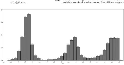
We follow Dehejia and Wahba (1999) and Becker and Ichino (2002) in obtaining empirical estimations. First, because, as shown by Horowitz (1993) and Newey, Powell, and Walker (1990), there is little difference in predicting outcomes using parametric or semiparametric methods, we estimate the propen-sity score by running a binary probit estimation givenwi. This step provides us with the estimated propensity score, pˆ(wi), which we can use to plot histograms for both the treatment and the control groups. We draw the histograms shown in Fig-ures1and2by focusing on a range of propensity score of 0.05– 0.45, because both the treated and control units are presented in this region. Table4gives the values calculated for ATE, ATET, and their associated standard errors. Four different ranges of
Figure 1. Treatment group. Histograms of estimated propensity scores in the overlapping region.
Damrongplasit, Hsiao, and Zhao: Decriminalization and Marijuana Smoking Prevalence 353
Figure 2. Control group. Histograms of estimated propensity scores in the overlapping region.
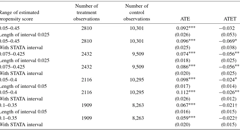
overlapping region (i.e., 0.05–0.45, 0.075–0.425, 0.05–0.4, and 0.1–0.35) and two different ways of partitioning the propen-sity scores (i.e., interval lengths 0.025 and 0.05) are consid-ered in this study. In addition to our manual partition, we also use STATA’spscorecommand to divide propensity scores into smaller stratums. The results given in Table4demonstrate that ATE varies between 0.059 and 0.112, while ATET fluctuates between −0.069 and −0.021. Because both ATE and ATET are highly sensitive to how the propensity score is stratified, we check whether condition (5.3) is met by testing for any dif-ference in the first moment between the treatment and control groups for each interval. Regardless of how we or STATA
par-tition the propensity score, thet-test and thet-squared test al-ways rejects the null hypothesis of means’ equality between the treatment and the control groups. This result suggests that con-ditioning on the propensity score, the distribution ofwiis differ-ent between the treated and the control units, implying a viola-tion of the balancing condiviola-tion. This violaviola-tion could be a result of sample size not being large enough for performing reliable nonparametric estimates, or because conditional independence assumption does not hold. Thus our propensity score matching estimates of the ATE and ATET could capture not only the treat-ment effect, but also the impact of differences in observable and unobservable covariates on smoking outcome.
Table 4. ATE and ATET using propensity score stratification method
Number of Number of Range of estimated treatment control
propensity score observations observations ATE ATET 0.05–0.45 2810 10,301 0.092∗∗∗ −0.032 Length of interval 0.025 (0.026) (0.053)
0.05–0.45 2810 10,301 0.096∗∗∗ −0.069∗ With STATA interval (0.025) (0.038)
0.075–0.425 2432 9,509 0.074∗∗∗ −0.056∗∗ Length of interval 0.025 (0.018) (0.025)
0.075–0.425 2432 9,509 0.086∗∗∗ −0.056∗∗ With STATA interval (0.020) (0.025)
0.05–0.4 2116 10,295 0.098∗∗∗ −0.024∗ Length of interval 0.05 (0.017) (0.014)
0.05–0.4 2116 10,295 0.112∗∗∗ −0.026∗∗ With STATA interval (0.026) (0.012)
0.1–0.35 1909 8,263 0.067∗∗∗ −0.021† Length of interval 0.05 (0.016) (0.015)
0.1–0.35 1909 8,263 0.059∗∗∗ −0.022† With STATA interval (0.020) (0.015)
NOTE: (i) *** significant at 1%, (ii) ** significant at 5%, (iii) * significant at 10%, (iv) † significant at 10% one-tailed test, (v) standard errors are in the parentheses.
354 Journal of Business & Economic Statistics, July 2010
6. SPECIFICATION ANALYSES
Our numerical analyses using parametric and nonparamet-ric methods yield very different inferences regardingthe impact of decriminalization on marijuana smoking prevalence. In this section we report specification analyses to investigate which model or method can more accurately capture the essentials of our data. As discussed in the previous section, our propen-sity score matching analysis fails to satisfy the balancing condi-tion implied by the condicondi-tional independence assumpcondi-tion, pos-sibly due to a violation of the conditional independence as-sumption. In contrast, the parametric approach can take into account of both selection on observables and unobservables si-multaneously, provided that the model’s assumptions are con-sistent with the data-generating process. If the parametric form is misspecified, then inference based on parametric specifica-tion can be misleading. For this reason, we first conduct a non-parametric kernel consistent test of the null of unrestricted en-dogenous probit switching model against the nonparametric al-ternative that does not place a restriction on the functional form or make any distributional assumptions. If the endogenous pro-bit switching model is not rejected, then we conduct likelihood ratio tests to choose between the unrestricted endogenous pro-bit switching model and its nested binary propro-bit model, sam-ple selection model, two-part model, and restricted endogenous switching model.
6.1 Parametric versus Nonparametric Modeling
Our maintained hypothesis for a parametric model is the un-restricted endogenous probit switching model that nests the re-stricted endogenous switching model, two-part model, sample selection model, and dummy variable model as special cases. The data-generating process could possibly follow other alter-native specifications, however. To check the adequacy of our unrestricted endogenous switching model in capturing the es-sential characteristics of the observed data, we test the null of the unrestricted endogenous switching model against the depar-ture from the null in any direction.
The basic idea of Bierens (1982), Hong and White (1995), and others on testing a parametric null of yi=m(xi, β)+ui against the departure from the null in any direction is that un-der the null H0:E(ui|xi)=0, whereas under the alternative, H1:E(ui|xi)=0. TestingE(ui|xi)=0 is equivalent to testing
E{uiE(ui|xi)f(xi)} =0. (6.1) Because ourxcontains both continuous and discrete variables, following Hsiao, Li, and Racine (2007) and Li and Racine (2007), we use
wherexcandxddenote continuous and discrete variables,qand rdenote the dimensions of continuous and discrete regressors, k(·) denotes the normal kernel function, andl(·) denotes the
whenxdi is an unordered discrete regressor and
l(xdis,xdjs, λs)=1 ifxdis=xdjs and Hsiao, Li, and Racine (2007) showed that under the null,
Jn=n(h1· · ·hq)1/2In/ But underH0,Jnconverges to the standard normal distribution at the slow rate ofOp((h1· · ·hq)1/2). To overcome this slow convergence problem, we use the following bootstrapping pro-cedure to approximate the finite-sample distribution of (6.6):
(i) From maximum likelihood estimatesβˆ1,βˆ0,αˆ1,αˆ0,γ ,ˆ
the dependent variable from bootstrapping,xi denotes the explanatory variables from the original data, n is the number of observations (14,008 in our case), andybi is drawn randomly from the binomial distribution with p= ˆp11i ifdi=1 andp= ˆp10i ifdi=0.
(iii) Use the bootstrapping samples{ybi,xi}ni=1from step (ii) to estimate the endogenous probit switching model [i.e., model (2.1)–(2.6)] by the maximum likelihood method and obtain a new set ofβˆ1b,βˆ0b,αˆ1b,αˆb0,γˆb,ρˆ1bυ, andρˆ0bυ.
Damrongplasit, Hsiao, and Zhao: Decriminalization and Marijuana Smoking Prevalence 355
(iv) Use the maximum likelihood estimatorsβˆ1b,βˆ0b,αˆb1,αˆ0b,
ˆ
γb,ρˆ1bυ, andρˆ0bυ from step (iii) and the bootstrapping samples{ybi,xi}ni=1from step (ii) to compute bootstrap-ping residualuˆbi and computeJnbusing the ad hoc plug-in bandwidthhs=(1.06)σs(n)−1/(2p+l), wherep is the order of the kernel function,ldenotes the dimension of continuous regressors, andσsis the sample standard de-viation for variables. We setλs=0 for discrete regres-sors.
(v) Repeat steps (ii)–(iv) 399 times and use the sorted test statistics, {Jnjb}399j=1, to construct a bootstrap empirical distribution, which in turn is used to approximate the null distribution of the test statisticJn.
We conduct a two-sided test by comparingJnwith the 1%, 5%, and 10% critical values from the bootstrap empirical dis-tribution. The two-sided critical values are 2.71 at 1%, 1.995 at 5%, and 1.625 at 10%, and Jn=1.282. In other words, it does not appear that our endogenous probit switching model is contradicted by the information contained in the data.
6.2 Likelihood Ratio Tests for Nested Alternatives
Taking the unrestricted endogenous probit switching model (2.1)–(2.6) as the maintained hypothesis and treating other parametric models as nested hypotheses, it follows that (a) if
H0∗:ρ1υ=ρ0υ=0, (6.8)
then the model becomes the restricted endogenous probit switching model; (b) if
H0∗∗:ρ1υ=ρ0υ=0, (6.9)
then the model has the form of a generalized two-part model; (c) if
H0∗∗∗:β1=β0 and ρ1υ=ρ0υ, (6.10)
then the unrestricted endogenous switching model is reduced to the sample selection model (Amemiya1985); and (d) if
H∗∗∗∗0 :β1=β0 and ρ1υ=ρ0υ=0, (6.11)
then the unrestricted endogenous switching model is reduced to the conventional dummy variable approach [model (2.7)]. To conduct specification tests forH0∗,H∗∗0 ,H0∗∗∗, andH∗∗∗∗0 , we compute likelihood ratio statistics, LR1, LR2, LR3, and LR4, respectively. Each is associated with different degrees of free-dom.
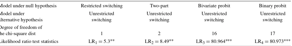
Table5presents the results of this specification analysis. LR2 and LR4 firmly reject the independence assumption between
the errors of the marijuana smoking equation and the errors of the residential choice equation, while LR1 demonstrates that the correlation of these error terms differ for the treatment and control groups. LR3and LR4also indicate that individuals do behave differently if marijuana smoking is decriminalized. In other words, our specification analysis appears to favor the un-restricted endogenous probit switching model.
7. CONCLUSION
In this work, we have used the 2001 wave of the NDSHS to empirically examine the impact of marijuana decriminaliza-tion on marijuana smoking prevalence in Australia. We used both parametric and nonparametric approaches. The advantage of the nonparametric approach is that it requires no functional form or distributional assumptions; the disadvantage is that the conditional independence assumption (i.e., ignorable treatment assignment assumption) is a maintained hypothesis. Further-more, the impacts of other sociodemographic effects on mar-ijuana smoking are not estimated. The advantage of parametric specification is that the issues of selection of both observables and unobservables can be taken into account, and the impact of each variable on outcome can be assessed provided that the parametric assumptions are not contradicted by information in the data. The disadvantage is that both functional form and dis-tributional assumptions are imposed. If these assumptions are incorrect, then the resulting inferences will be misleading. But our data analysis appears to indicate that the validity of the con-ditional independence assumption for nonparametric matching adjustment is contradicted by the information in the data. In contrast, our parametric model does not appear to be contra-dicted by the information in the data. In fact, the world is not that benevolent. We could be asking too much of our data. As noted by Griliches (1967, pp. 17–18), “we want them to test our theories, provide us with estimates of important parameters, and disclose to us the exact form of the interrelationships be-tween the various variables.” When the information contained in the data is limited, an integration of behavioral assumption and parametric specification may allow us to extract more use-ful information from the data.
Conditional on a state’s decriminalization status, our speci-fication analysis appears to favor the unrestricted endogenous probit switching model that takes into account both selection on observables and unobservables. This model suggests that a decriminalization policy leads to greater marijuana smoking participation. It indicates that on average, living in a decrimi-nalized state significantly increases the probability of smoking marijuana, by 16.2%. This estimate is higher than the estimates
Table 5. Likelihood ratio tests
Model under null hypothesis Restricted switching Two-part Bivariate probit Binary probit Model under Unrestricted Unrestricted Unrestricted Unrestricted alternative hypothesis switching switching switching switching Degree of freedom of
the chi-square dist 1 2 16 17
Likelihood ratio test statistics LR1=5.3∗∗ LR2=8.49∗∗ LR3=80.964∗∗∗ LR4=80.973∗∗∗
NOTE: (1) *** significant at 1% (two-tailed test), (2) ** significant at 5% (two-tailed test).
356 Journal of Business & Economic Statistics, July 2010
obtained from the dummy variable approach, the sample selec-tion model, the two-part model, and previous studies. The dis-crepancies could be due to the use of different data sets or to differing model specifications, as demonstrated in the present study. Our specification analysis appears to favor the model that allows both endogeneity of the decriminalization dummy and flexibility of different behavioral patterns due to changes in the legal or institutional environment.
ACKNOWLEDGMENTS
The authors thank Ragui Assaad, Deborah Levison, and Cristobal Ridao-Cano for the use of their maximum likelihood computer program and Jeffrey Racine for the use of his R pro-gram to conduct the specification analysis. They also thank two referees, an editor, and John Ham, Qi Li, Chiahui Lu, Jeffrey Nugent, Michael Nichols, John Strauss, and Vai-Lam Mui for their helpful comments.
[Received November 2006. Revised January 2009.]
REFERENCES
ABCI (2002), “Australia Illicit Drug Report,” discussion paper, Australia Bu-reau of Criminal Intelligence. [347]
ABS (2003a), “Consumer Price Index 14th Series: By Region, All Groups,” Cat. No. 640101b, Australia Bureau of Statistics. [348]
(2003b), “Australian National Accounts: State Accounts,” Cat. No. 5220.0, Australia Bureau of Statistics. [348]
ACC (2003), “Australia Illicit Drug Report,” Report 2001-02, Australia Crime Commission. [347]
Amemiya, T. (1985),Advanced Econometrics, Cambridge, MA: Harvard Uni-versity Press. [346,355]
Becker, S., and Ichino, A. (2002), “Estimation of Average Treatment Effects Based on Propensity Scores,”Stata Journal, 2, 358–377. [352]
Becker, G., and Murphy, K. (1988), “A Theory of Rational Addiction,”Journal of Political Economy, 96, 675–700. [347]
Bierens, H. (1982), “Consistent Model Specification Tests,”Journal of Econo-metrics, 20, 105–134. [354]
Cameron, C., and Trivedi, P. (2005),Microeconometrics: Methods and Appli-cations, New York: Cambridge University Press. [352]
Cameron, L., and Williams, J. (2001), “Cannabis, Alcohol and Cigarettes: Sub-stitutes or Complements?”The Economic Record, 77, 19–34. [345,348] Caneiro, P., Hansen, K., and Heckman, J. (2003), “Estimating Distributions of
Treatment Effects With an Application to the Returns to Schooling and Measurement of the Effects of Uncertainty on College Choice,” Interna-tional Economic Review, 44, 361–422. [345]
Clements, K. (2004), “Three Facts About Marijuana Prices,”The Australian Journal of Agricultural and Resource Economics, 48, 271–300. [348] Dehejia, R., and Wahba, S. (1999), “Causal Effects in Nonexperimental Studies:
Reevaluating the Evaluation of Training Programs,”Journal of the Ameri-can Statistical Association, 94, 1053–1062. [352]
DiNardo, J., and Lemieux, T. (2001), “Alcohol, Marijuana, and American Youth: The Unintended Consequences of Government Regulation,” Jour-nal of Health Economics, 20, 991–1010. [345]
Duan, N., Manning Jr., W., Morris, C., and Newhouse, J. (1983), “A Compar-ison of Alternative Models for the Demand for Medical Care,”Journal of Business & Economic Statistics, 1, 115–126. [346]
(1984), “Choosing Between the Sample-Selection Model and the Multi-Part Model,”Journal of Business & Economic Statistics, 2, 283–289. [346]
Feridhanusetyawan, T., and Kilkenny, M. (1996), “Rural/Urban Residence Lo-cation Choice,” working paper, Iowa State University, Center for Agricul-tural and Rural Development. [347]
Griliches, Z. (1967), “Distributed Lag: A Survey,”Econometrica, 35, 16–49. [355]
Heckman, J., and Robb, R. (1985), “Alternative Methods for Evaluating the Impact of Interventions,” inLongitudinal Analysis of Labor Market Data, eds. J. Heckman and B. Singer, New York: Cambridge University Press. [352]
Hong, Y., and White, H. (1995), “Consistent Specification Testing via Nonpara-metric Series Regression,”Econometrica, 63, 1133–1159. [354]
Horowitz, J. (1993), “Semiparametric and Nonparametric Estimation of Quan-tal Response Models,” inHandbook of Statistics, Vol. 11, eds. G. Maddala, C. Rao, and H. Vinod, Amsterdam: North-Holland. [352]
Hsiao, C. (1983), “Identification,” inHandbook of Econometrics, Vol. 1, eds. Z. Griliches and M. Intriligator, Amsterdam: North-Holland. [346,347] Hsiao, C., Li, Q., and Racine, J. (2007), “A Consistent Model Specification Test
With Mixed Discrete and Continuous Data,”Journal of Econometrics, 140, 802–826. [354]
Keane, M., and Wolpin, K. (1997), “The Career Decisions of Young Men,” Journal of Political Economy, 105, 473–522. [345]
Kittiprapas, S., and McCann, P. (1999), “Industrial Location Behaviour and Regional Restructuring Within the Fifth Tiger Economy: Evidence From the Thai Electronics Industry,”Applied Economics, 31, 37–51. [347] Li, Q., and Racine, J. (2007),Nonparametric Econometrics Theory and
Prac-tice, Princeton, NJ: Princeton University Press. [354]
Moore, T. (2005), “Australian Government Spending Estimates,” Bulletin No. 2, DPMP Bulletin Series, Turning Point Alcohol and Drug Centre, Fitzroy, Melbourne. [344]
NDSHS (2001), Computer data files, National Drug Strategy Household Sur-veys 2001, Social Science Data Archives, Australian National University, Canberra. [345,347]
Newey, W., Powell, J., and Walker, J. (1990), “Semiparametric Estimation of Selection Models: Some Empirical Results,”American Economic Review, 80, 324–328. [352]
Pacula, R. (1998), “Does Increasing the Beer Tax Reduce Marijuana Consump-tion?”Journal of Health Economics, 17, 557–585. [345,347,348] Pacula, R., Chriqui, J., and King, J. (2003), “Marijuana Decriminalization:
What Does It Mean in the United States?” Working Paper 9690, NBER. [345]
Quandt, R. (1972), “A New Approach to Estimating Switching Regressions,” Journal of the American Statistical Association, 67, 306–310. [346] Rosenbaum, P., and Rubin, D. (1983), “The Central Role of the Propensity
Score in Observational Studies for Causal Effects,”Biometrika, 70, 41–55. [352]
Saffer, H., and Chaloupka, F. (1995), “The Demand for Illicit Drugs,” Working Paper 5238, NBER. [345]
(1998), “Demographic Differential in the Demand for Alcohol and Illicit Drugs,” Working Paper 6432, NBER. [345,348]
Thies, C., and Register, C. (1993), “Decriminalization of Marijuana and the Demand for Alcohol, Marijuana, and Cocaine,”The Social Science Journal, 30, 385–399. [345,348]
Williams, J. (2004), “The Effects of Price and Policy on Marijuana Use: What Can Be Learned From the Australian Experience?”Health Economics, 13, 123–137. [345,347,348]
Zhao, X., and Harris, M. (2004), “Demand for Marijuana, Alcohol and To-bacco: Participation, Levels of Consumption, and Cross-Equation Correla-tions,”Economic Record, 80 (251), 394–410. [345,347,348]