Full Terms & Conditions of access and use can be found at
http://www.tandfonline.com/action/journalInformation?journalCode=ubes20
Download by: [Universitas Maritim Raja Ali Haji] Date: 11 January 2016, At: 23:19
Journal of Business & Economic Statistics
ISSN: 0735-0015 (Print) 1537-2707 (Online) Journal homepage: http://www.tandfonline.com/loi/ubes20
Sequential Bayesian Analysis of Time-Changed
Infinite Activity Derivatives Pricing Models
Junye Li
To cite this article: Junye Li (2011) Sequential Bayesian Analysis of Time-Changed Infinite Activity Derivatives Pricing Models, Journal of Business & Economic Statistics, 29:4, 468-480, DOI: 10.1198/jbes.2010.08310
To link to this article: http://dx.doi.org/10.1198/jbes.2010.08310
Published online: 24 Jan 2012.
Submit your article to this journal
Article views: 299
Sequential Bayesian Analysis of Time-Changed
Infinite Activity Derivatives Pricing Models
Junye L
IDepartment of Finance, ESSEC Business School, 188064 Singapore (li@essec.edu)
This article investigates time-changed infinite activity derivatives pricing models from the sequential Bayesian perspective. It proposes a sequential Monte Carlo method with the proposal density generated by the unscented Kalman filter. This approach overcomes to a large extent the particle impoverishment problem inherent to the conventional particle filter. Simulation study and real applications indicate that (1) using the underlying alone cannot capture the dynamics of states, and by including options, the pre-cision of state filtering is dramatically improved; (2) the proposed method performs better and is more robust than the conventional one; and (3) joint identification of the diffusion, stochastic volatility, and jumps can be achieved using both the underlying data and the options data.
KEY WORDS: Infinite-activity jumps; Option pricing; Sequential Monte Carlo method; State filtering; Stochastic volatility; Unscented Kalman filter.
1. INTRODUCTION
In contrast to the compound Poisson process, infinite-activity Lévy processes can generate an infinite number of jumps within any finite time interval, capturing not only the rarely occurring large jumps, but also the frequently occurring small jumps. Be-cause of this flexible feature, they have been attracting increas-ing attention and becomincreas-ing more popular for modelincreas-ing asset prices both in academics and in practice. Even though investi-gation of the parameter estimation problem for these models is very intensive, little attention has been paid to the efficient state filtering issue.
In financial applications, we are actually more interested in the sequential study of the model. First, people in the market have to estimate and forecast latent factors in real time. For ex-ample, one needs to recursively estimate and forecast volatility for option pricing and risk management whenever a new ob-servation arrives. Second, people need to sequentially disentan-gle different factors and to study their influence on asset price dynamics. Third, the sequential method dramatically reduces computational cost in comparison with batch estimation, which has to restart the estimation procedure every time new data ar-rive. Furthermore, the sequential method naturally produces the filtering density that is crucial for constructing the likelihood function and implementing parameter estimation. Some work has been published on sequential Bayesian analysis and effi-cient state filtering for stochastic volatility and jump-diffusion models (Stroud, Muller, and Polson 2003; Johannes, Polson, and Stroud2009). Not much work has yet been done on infinite-activity Lévy models, however.
If the infinite-activity derivatives pricing models can be trans-formed into into the dynamic state-space model (DSSM) frame-work, then the sequential estimation via Bayesian filtering can be applied. The DSSM can be written in the following form:
yt=H(xt, ,wt), (1)
xt=F(xt−1, ,vt), (2)
where the observationyt is assumed to be conditionally inde-pendent given the statextwith the distributionp(yt|xt); the state xt is modeled as a Markov process with the initial distribution
p(x0)and the transition lawp(xt|xt−1);wt andvt are
indepen-dent observation noise and state noise with mean 0 and variance
RwandRv, respectively; andis a set of static parameters.
Based on previous and current observations, filtering is a process of estimating a system’s current state, that is, finding the posterior distribution,p(xt|y1:t), from which inference can
be made. By Bayes’s rule, the posterior distributionp(xt|y1:t)
can be computed through
p(xt|y1:t)=
p(yt|xt)p(xt|y1:t−1) p(yt|y1:t−1)
. (3)
Thus, calculation and/or approximation of the priorp(xt|y1:t−1), of the likelihoodp(yt|xt)and of the evidencep(yt|y1:t−1)is the essence of Bayesian filtering and inference.
If functionsH(·)andF(·)are linear and if Gaussian distri-butions are assumed for xt, wt, and vt, then the well-known Kalman filter can be applied, and the optimal solution is obtain-able. When the model becomes nonlinear and Gaussian, non-linear Kalman filters can still be used efficiently. Unfortunately, all of the infinite-activity derivatives pricing models are nonlin-ear and non-Gaussian. For recursive estimation of these models, sequential Monte Carlo methods (also known as particle filters) are good choices. Particle filters were formally established by Gordon, Salmond, and Smith (1993) and further developed by many others. The basic idea of particle filters is to represent distributions of all random variables with a number of parti-cles (samples) drawn directly from the state space and update them using the sequential importance sampling and resampling method.
One critical problem in implementing particle filters is how to optimally design a proposal density. The conventional par-ticle filter (Gordon, Salmond, and Smith 1993) takes the state transition law as the proposal density for its ease of implemen-tation. Because the proposal density does not take the latest observation into account, it is easy for this method to be de-generate. The introduction of jumps and the highly nonlinear
© 2011American Statistical Association Journal of Business & Economic Statistics
October 2011, Vol. 29, No. 4
DOI:10.1198/jbes.2010.08310
468
derivatives pricing formula in continuous-time financial mod-els makes the situation even worse. There are two ways to de-sign a better proposal density. One approach improves the algo-rithm’s efficacy by using an auxiliary variable (Pitt and Shep-hard1999), and the other addresses the degeneracy problem directly by incorporating the latest information. In this arti-cle I take the latter approach and propose a sequential Monte Carlo method with the proposal density generated by the un-scented Kalman filter based on the method of van der Merwe et al. (2000).
The unscented Kalman filter (UKF), recently developed in the field of engineering (Julier and Uhlman1997,2004), uses deterministic sampling approaches to approximate sufficient statistics of the nonlinear Gaussian system. The idea behind this approach is that to estimate the state information after a non-linear transformation, it is favorable to approximate the prob-ability distribution directly instead of linearizing the nonlinear functions. The unscented Kalman filter overcomes to a large ex-tent the pitfalls inherent to other nonlinear Kalman filters, such as the extended Kalman filter, and improves the accuracy and robustness of estimation without increasing the computational cost. However, the UKF has the limitation that it cannot be ap-plied to general non-Gaussian models.
For recursive estimation of the infinite-activity Lévy mod-els, I introduce the unscented sequential Monte Carlo method, which uses the UKF to generate the sophisticated proposal den-sity by taking into account the latest information and then ap-plies the particle filter to handle the nonlinear and non-Gaussian systems. To be concrete, I apply the UKF to each particle for update and propagation and then compute the optimal filtering density. Even though the Gaussian assumption is not realistic for the infinite-activity derivatives pricing models, it is less of a problem to generate each individual particle with a distinct mean and variance. Furthermore, because the UKF directly uses the nonlinear functions and approximates the posterior mean and covariance with accuracy at least up to the second order, the nonlinearity of the system is well preserved.
I report a simulation study and real data applications to de-termine the performance of the proposed method with compar-ison to the conventional approach, and answer the following questions. First, is it helpful for state filtering to incorporate derivatives in the observation set? I investigate the informa-tion content contained in the underlying and the derivatives and the different roles played by these. Second, can the proposed algorithm capture jumps realized by the infinite-activity Lévy processes? Finally, is it feasible to jointly identify the diffusion, stochastic volatility, and infinite-activity jumps? Joint identifi-cation is important for derivative pricing and risk management, because the tail behavior of the distribution of asset returns is determined mainly by jumps, especially by large jumps.
This article is the first to fully investigate the time-changed infinite-activity derivatives pricing models from the sequen-tial Bayesian perspective and is also one of the first to ap-ply the unscented filtering methods to finance. It parallels the work ofJohannes, Polson, and Stroud(2009) that studied the jump-diffusion stochastic volatility models with conventional and auxiliary particle filters. The algorithm proposed in this ar-ticle performs better, especially for large-jump and multifactor stochastic volatility models, and is more robust than the con-ventional particle filter, which cannot effectively capture the
dynamics of states in the time-changed infinite-activity Lévy models, especially in real data applications.
The rest of the article is organized as follows. Section 2
builds the infinite-activity derivatives pricing model and con-structs the corresponding state-space representation. Section3
discusses the sequential Monte Carlo method with the proposal density generated by the UKF. Section4implements a simula-tion study. Secsimula-tion5presents applications using the S&P 500 index and index options. Section6concludes.
2. DYNAMIC STATE–SPACE MODEL FRAMEWORK
2.1 Infinite-Activity Lévy Process and Derivatives Pricing Model
Under a given probability space(,F,P), and the complete filtrationFt, a Lévy process, Xt is acadlagstochastic process
with independent and stationary increments andX0=0. By the Lévy–Kintchine theorem, the characteristic function ofXt has
the following form:
φX(u)=E[eiuXt] =e−tψX(u), (4)
whereψX(u)is termed the characteristic exponent,
ψX(u)= −iuμ+ measures the arrival rate of jumps with sizexdefined onR0(real line without 0). A Lévy process exhibits infinite activity when
R0
v(x)dx= ∞. (6)
Otherwise, it is a finite-activity process. The infinite-activity Lévy process can generate an infinite number of jumps at any finite time interval, whereas the finite-activity process can gen-erate only a finite number of jumps within any finite time inter-val.
The derivatives pricing model is built by taking into ac-count both jumps and stochastic volatility in the underlying as-set process. Jumps are modeled by the infinite-activity Lévy process, and stochastic volatility is introduced through time-changing stochastic processes (Clark1973; Carr et al.2003).
Define a stopping time, Tt, given a nonnegative and
right-continuous with left limit stochastic process Vt under the
de-fined probability space
Tt=
t 0
Vs−ds,
which is finite almost surely. Intuitively, we can viewtas cal-endar time andTtas business time. The variableVtreflects the
intensity of economic activity and is termed the variance rate. Stochastic volatility is generated by replacing the calendar time
twith the business timeTt.
A well-known nonnegative stochastic process is the square-root process (Cox, Ingersoll, and Ross1985), which is used to
model the variance rate process. The asset price is then mod-eled with the exponential time-changed Brownian motion and infinite-activity Lévy process
whereWt is a Brownian motion,Xt is an infinite-activity Lévy process that captures both the frequently occurring small jumps and the rarely occurring large jumps; Tt(1) and Tt(2) are two
stochastic business times used to generate stochastic volatil-ity from Wt andXt, respectively; Vt(1) and V
(2)
t are variance
rates to construct the stochastic business times,Z(t1), and Zt(2)
are Brownian motions that are independent of one another; r
is a constant risk-free interest rate; andπW andπXcapture the
diffusion and jump risk premia, respectively.
Z(t1)is allowed to be correlated toWtwith a correlation
para-meter,ρt, to accommodate the leverage effect and is indepen-dent ofXt.Zt(2)is independent of bothWtandXt.kX(1)is the
convexity adjustment derived from the cumulant exponent of
Xt:k(s)≡1t log(E[esXt])= −ψX(−is).
Assume that there exists an equivalent martingale measure
Q, under which the risk-neutral model is defined as
St=S0exprt+WQ stochastic volatility are introduced to financial modeling, the market becomes incomplete, and many different risk-neutral measures may exist. I assume that the change of measure does not alter the structure of stochastic processes, and that this can be done using the well-known Esscher transform,
dQ cumulant exponent ofYt. Under the equivalent martingale
mea-sure, the new Lévy density is just an exponential tilting of the objective densityv˜(dy)=e−ξyv(dy). Exponential tilting mainly affects large jumps. This is consistent with our understanding of
financial market movements, in which large jumps have a dom-inant influence on option pricing and risk management. The Esscher transform gives an equivalent martingale measure,Q, which has the minimum relative entropy with respect to the ob-jective measureP. Intuitively, this means thatQis an equivalent martingale measure that is the closest toP in terms of infor-mation content (Chan1999). Under the Esscher transform, the risk premium is given byπY=k(1)−kQ(1)(Gerber and Shiu 1994).
For this risk-neutral model, the conditional characteristic function of log returnsRt=ln(St/St−τ)can be derived using approaches of Duffie, Pan, and Singleton (2000) and Carr and Wu (2004). It has the following form:
φR(u;τ,Vt−τ)≡EQ[eiuRt|Ft−τ]
wherei=1,2,ψXQis the characteristic exponent of the infinite activity Lévy process under the risk-neutral measure, andkQX(·) is its cumulant exponent. With this conditional characteristic function, we can compute European-type derivative prices with the fast Fourier transform method (Carr and Madan1999). In this article I use a more efficient algorithm, the fractional fast Fourier transform (Chourdakis2005).
This time-changed infinite activity model is very general and contains many models that appear in the literature. Huang and Wu (2004), Bakshi, Carr, and Wu (2008), and Li, Favero, and Ortu (2009) investigated this kind of infinite-activity Lévy model from the batch estimation perspective.Li, Favero, and Ortu (2009) also investigated the double-jump model by in-troducing a jump component in the variance rate process and found that whenever the underlying asset is modeled with an infinite-activity Lévy process, the introduction of jumps in the variance rate process is not critically important. Thus I do not consider volatility jumps in this article.
2.2 State-Space Representation
To study the model with Bayesian filtering methods, I need to construct an appropriate state-space representation.
First, I decorrelate the underlying and variance rates for ap-plicability of Bayesian filtering methods. For the time-changed Brownian motion, we have
where d indicates the equivalence in distribution. With this property and the fact that[dWt,dZt(1)] =ρdt, I rewrite the
un-derlying process (7) and the variance rate process (9) as follows:
lnSt=lnS0+rt+
which can be considered an observation equation. Now we can see that the observation noise in (19) and the state noise in (9) are independent.
Second, because most of infinite-activity Lévy processes en-countered in finance have tractable Brownian subordination forms, I take advantage of this property and regard the jump as one of the states
X
Tt(2)=ωSt+ηW˜(St), (20)
whereStis the subordinator under the business time and is also
taken as one state,St=gS(Tt(2);), where are parameters
of the distributiongS.
Finally, discretizing the model with a time interval τ and also taking into consideration derivatives leads to the follow-ing state-space representation:
where derivatives are assumed to be collected with measure-ment errors ǫOt →N(0, σO2), independent of wt, zt, and w˜t,
which also are mutually independent standard normal white noise; St and yOt are the discretely observed underlying and
derivative prices; f(·) is the theoretical derivative price com-puted from the model; and the variance rates Vt(1) and Vt(2), jump sizeXt, and jump timeStare regarded as states.
For the small time interval τ, such as daily or higher fre-quency, discretization of continuous-time models does not in-troduce significant bias in estimation (Eraker, Johannes, and Polson 2003; Johannes, Polson, and Stroud 2009). With this state-space representation, we can apply sequential Monte Carlo methods to state filtering.
3. UNSCENTED SEQUENTIAL BAYESIAN METHOD
The infinite-activity derivatives pricing model introduced in Section2is obviously nonlinear and non-Gaussian. Direct use of the unscented Kalman filter is inefficient because of its lim-itation of Gaussian assumptions. Thus I propose the applica-tion of sequential Monte Carlo methods (i.e., particle filters) that approximate the posterior distribution of states by a set of weighted particles (i.e., samples) without making any ex-plicit assumptions and can be applied to any nonlinear and non-Gaussian systems. Since their introduction by Gordon, Salmond, and Smith(1993), particle filters have been success-fully used in many fields, but their application to financial prob-lems has not attracted much attention. To improve the efficiency on the conventional particle filter and avoid the sample impov-erishment problem, I introduce the unscented sequential Monte Carlo method, which uses the unscented Kalman filter to gen-erate the proposal density by taking into account the latest in-formation and then applies the particle filter to handle the non-Gaussian systems. In this section, I first introduce the UKF and then discuss the unscented sequential Monte Carlo method.
3.1 Unscented Kalman Filter
The unscented Kalman filter is proposed to improve the effi-ciency of Gaussian approximation algorithms. It is a straightfor-ward application of the scaled unscented transformation, which uses the so-called “sigma points” to cover and propagate infor-mation on data. The scaled unscented transforinfor-mation can ap-proximate posterior mean and covariance of a random variable undergoing a nonlinear transformation with accuracy up to the second order and the third order for a Gaussian prior (Julier and Uhlman 1997,2004). The unscented Kalman filter is derived
based on the scaled unscented transformation. The unscented Kalman filter does not explicitly approximate or linearize the nonlinear observation and state models. It uses true nonlinear models and updates state variables through a set of determinis-tic sigma points generated by the unscented transformation.
Consider a nonlinear function y=f(x), with mean and co-variance of the random variablex(with dimensionL) ofx¯and
Px. The idea of the unscented transformation is that the mean
and covariance ofycan be computed by forming a set of 2L+1 αdetermines the spread of sigma points aroundx¯ and is usu-ally set to be a small positive value, andκ is a second scaling parameter with value set to 0 or 3−L. These sigma points are propagated through the nonlinear functionf,
Yi=f(χi), i=0,1, . . . ,2L. (24)
The mean and covariance of y are then approximated with a weighted sample mean and covariance of posterior sigma points, where superscripts (m) and(c)indicate that weights are for construction of the posterior mean and covariance, respectively, andβ is a covariance correction parameter used to incorporate prior knowledge of the distribution ofx. Typical values forκ, α, andβ are 0, 10−3, and 2, respectively. These values should suffice for most purposes.
The unscented Kalman filter relies on the scaled unscented transformation. Suppose for the moment that the DSSM (1) and (2) arenonlinear Gaussian. We first concatenate the state, the observation noise, and the state noise at timet−1,
xet−1=[xt−1 wt−1 vt−1]′, (28) whose dimension is L=Lx+Lw+Lv, with Lx, Lw, and Lv
being dimensions of the state, the observation noise, and the state noise, respectively, with mean and covariance
ˆ
I then use the scaled unscented transformation to form a set of 2L+1 sigma points,
and the corresponding weights. With these sigma points, the nonlinear Kalman filter is implemented as follows:
For the time update, and for the measurement update,
Yt|t−1=Hχtx|t−1, χtw|t−1
Then the posterior meanxˆt and posterior covariancePxt of the
statextcan be obtained.
3.2 Unscented Sequential Monte Carlo Method
My actual aim is to recursively estimate the posterior distrib-utionp(x0:t|y1:t)and in particular the filtering densityp(xt|y1:t),
given that the DSSM (1) and (2) are nonlinear and non-Gaussian. Because the UKF assumes Gaussian distributions, it results in an inefficient estimate in this setting. Thus I rely on the sequential Monte Carlo methods and take into account the latest observations when designing the proposal density.
Under some regularity conditions, sequential Monte Carlo Methods/particle filters approximate the filtering density
p(xt|y1:t)with the empirical point-mass estimatepˆ(xt|y1:t)
wherew˜(ti) is the normalized importance weight for each par-ticle and δ(·) denotes the Dirac delta function. As the num-ber of particles N increases, the accuracy of this approxima-tion improves, and the law of large number guarantees the con-vergence. Because it is usually impossible to sample directly from the posterior density function, we can apply the impor-tance sampling method and alternatively sample from a known and easily sampled proposal density functionπ. GivenN sam-ples{x(ti),i=1,2, . . . ,N}drawn from the proposal density, the
and the unnormalized weightwt can be recursively updated as
(see Doucet, de Freitas, and Gordon2001).
In principle, there are many choices of the proposal density as long as its support includes that of the posterior density and it is easy to sample. The most frequently used proposal density is the transition density of states. In implementation, this parti-cle filter usually meets the sample depletion problem, however; that is, after a few updating steps, only a small number of par-ticles have significant weights. A resampling stage is custom-arily included to overcome this problem. However, the main cause of sample depletion is the failure to move particles to high-likelihood regions, and this failure stems directly from the poor proposal density. Note that two critical factors are associ-ated with the proposal density: First, particles are drawn from the proposal density, and second, the proposal density is used to calculate each particle’s weight. Thus a good choice of the pro-posal densityπ(xt|x0:t−1,y1:t)plays a paramount role in particle
filters.
Doucet, Godsill, and Andrieu (2000) noted that the optimal proposal density, which should minimize the variance of impor-tance weights, has the following form:
π(xt|x0:t−1,y1:t)≡p(xt|xt−1,yt). (35) p(xt|xt−1,yt) does not usually have an analytical form, and the true value ofxt−1 is not known. All that is known about xt−1 is that the information reflected by xt−1 is summarized inp(xt−1|y1:t−1). Thus the optimal proposal density can be
ap-proximated by
p(xt|xt−1,yt)p(xt−1|y1:t−1)dxt−1=p(xt|y1:t), (36)
to which the Kalman filter-generated Gaussian approximation πN(xt|y1:t)can be applied.
The extended Kalman filter is the most commonly used non-linear Kalman filter. The extended Kalman filter performs very poorly for a highly nonlinear system, however. An alternative is the unscented Kalman filter described in Section3.1, which is more efficient than the extended Kalman filter. Thus I use the UKF to design the proposal density; that is, I approximate the optimal proposal density with a Gaussian density generated by the UKF for each particle. This proposal density takes into account the latest observation and can capture the complicated structure, such as multimodalities, skewness, and other high-order moments. Note that even though the Gaussian assumption is not realistic for the optimal densityp(xt|xt−1,yt), it is less of
a problem to generate each individual particle with a distinct mean and variance. Furthermore, because UKF approximates the mean and covariance of the posterior with accuracy at least up to the second order, the nonlinearity of the system is well preserved.
The algorithm comprises the following steps:
• Step 1: Initialize att=0. Draw a set of particles{x(0i),i=
1, . . . ,N}from the prior p(x0) and give each particle a weightN1.
• Step 2: Fort=1,2, . . .
– update the prior distribution for each particlex(ti−)1with the UKF, as discussed in the previous section, to obtain posterior meanx¯(ti)and varianceP(ti);
– samplex(ti)−→ ˜π (x(ti)|y1:t)≡N(¯x(ti),P
(i)
t );
– update the weight for each particle using the formula (34), with the denominator replaced by the proposal densityπ (˜ x(ti)|y1:t);
– normalize the weight,w˜(ti)=w(ti)/N
j w
(j)
t . • Step 3: Resample (residual sampling)
– retainNi′= ⌊Nw˜t(i)⌋copies ofx(ti); which are approximately distributed according to
p(xt|y1:t).
The algorithm says that the unknown posterior distribution of states can be approximated by a set ofproperly weighted parti-cles drawn from a known distributionπ˜ (Liu and Chen1998), which is generated by the UKF. The resampling step is used to eliminate the particles with low importance weights and to mul-tiply the particles with high importance weights. This is done by mapping the weighted measure,{x(ti),w˜(ti)}, to an unweighted measure,{x(ti),1/N}. At this step, I apply the residual resam-pling approach (Liu and Chen1998). I have experimented with other resampling schemes (multinomial and systematic resam-pling) and have found that the multinomial is dominated by the other two, and that results are not materially affected by the par-ticular choice between residual and systematic methods. After the resampling scheme,N particles approximately distributed according top(xt|y1:t)are obtained, from which inference can
be made; for example, the current states can be estimated by
ˆ
xt=N1Ni=1x (i)
t .
4. SIMULATION STUDY
In this section I implement a simulation study with the deriv-atives pricing model built on the variance gamma (VG) process (Madan, Carr, and Chang1998). The VG process has a tractable Brownian subordination form,Xt=ωSt+ηW(St), whereStis
the gamma process with the probability density
fG(x)=xt/v−1
1
vt/vŴ(t/v)e−
x/v. (37)
It is reparameterized to have unit mean rate and variance ratev, which mainly determines the jump structure. The characteristic exponent of the VG process can be derived as follows:
ψVG(u)=
For demonstration, I assume zero risk premia and setVt(2)=
1. More simulation results are provided on my website. In this setting, we have parameters = {ω, η,v, κ(1), θ(1), σ(1), ρ} and statesxt= {Vt(1),Xt,St}. In total, 500 daily data points are
simulated with the initial statesS0=100,V0=0.025,X0=0,
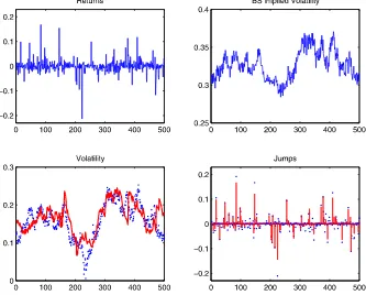
andS0=0 and the true parameters∗= {−0.04,0.30,0.05, 6.00,0.025,0.30,−0.50}. The simulated options data are those of at-the-money short maturity calls with the strike equal to the stock price and the maturity equal to 1 month. I assume that the risk-free interest rate is known and equal to 6%, and that option prices are contaminated by the measurement noise ǫtO→N(0, σO2). In what follow, I consider different values of σO. The upper panels of Figure1 present the simulated stock
returns and the Black–Scholes implied volatility of the simu-lated at-the-money options.
I first implement the proposed filtering algorithm using the stock price data alone to see whether stock prices contain enough information to effectively capture the dynamics of states. The number of particles is 3000. The lower panels of Figure1plot the filtered results of volatility and jumps. They show that the filtered jumps miss some large jump points, and that the filtered volatility clearly deviates from the true path.
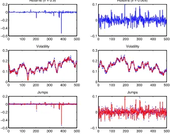
I then combine the data on stock prices and options and eval-uate whether the latter are helpful for state filtering. Option prices are contaminated by measurement errors withσO=7%,
and only 200 particles are used. The main observation is that the precision of state filtering has improved dramatically. The up-per panels of Figure2present the filtered volatility and jumps jointly using both datasets. The left upper panel presents the volatility paths, which show that the estimates are very similar to the true values. The right upper panel presents the filtered jumps. As shown, for the large jumps, the algorithm achieves nearly perfect results, and for the small jumps, the results are also very satisfactory. The algorithm can capture both the large jumps and the small jumps. This improvement originates from
the fact that options are forward-looking and contain richer in-formation on volatility and jump dynamics than stock prices.
I also investigate how the algorithm performs if the variance of the measurement error is increased. The lower panels of Fig-ure2 present the filtered volatility and jumps with σO set to
15%. The proposed method can still effectively capture the dy-namics of states even though the filtered results are a little noisy compared with previous results.
The parametervmainly determines the jump structure. Ifvis large, then the process generates many tiny jumps occasionally accompanied by huge jumps. In contrast, ifvis very small, then most jumps occur with size around the meanτ. I study these different cases and examine whether the proposed algorithm can capture the rich jump structure generated by the variance gamma process. Figure3presents the true and filtered volatility and jumps forv=0.50 and 0.005, respectively. The top panels show the simulated returns, and the lower two panels compare the filtered states and the true values. The robustness of the al-gorithm is apparent. For both volatility and jump filtering, the algorithm can capture the true values in both cases. What is more striking is that in the case wherev=0.5, the largest jump occurring around point 390 is successfully captured by the pro-posed method.
To check whether the method proposed in this article is su-perior to the conventional particle filter in the time-changed in-finite activity jump model, I also run the conventional particle filter with the proposal density being the state transition law for the three datasets generated before using both the underlying and derivative data. I find that it is impossible to obtain satis-factory filtering results if the same number of particles are used
Figure 1. Simulated data and state filtering using stock prices alone. The upper panels show the simulated stock returns (left) and the BS implied volatility of the simulated at-the-money call options (right). The lower panels present the filtered volatility (left) and jumps (right) obtained from the unscented sequential Monte Carlo method using the stock price data alone. The dots represent the true values, and the lines represent the estimated values. The number of particles is 3000. The online version of this figure is in color.
Figure 2. Joint state filtering. The figure presents the filtered volatility and jumps obtained from the unscented sequential Monte Carlo method using both the stock and the option prices. The upper panels present the filtered results with measurement errorσO=7%, and the lower panels present the filtered results with measurement errorσO=15%. The dots represent the true values, and the lines represent the estimates. The number of particles is 200. The online version of this figure is in color.
Figure 3. Simulated data and joint state filtering. Data are simulated with the same parameters as before except the parameterv. The top panels present the simulated returns. The lower two panels present the true (dots) and filtered (lines) volatility and jumps. The standard deviation of the measure error isσO=7%. The number of particles is 200. The online version of this figure is in color.
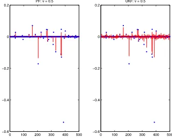
Figure 4. Joint state filtering: PF and UKF. The states are filtered using the stock and option prices with the conventional particle filter and the UKF. The figure presents the filtered jumps for the jump structurev=0.5. The dots are the true values, and the lines are filtered values. The number of particles is 3000 in the conventional particle filter. The online version of this figure is in color.
as before (200). Thus I increase the number of particles to 3000, so that the two algorithms have nearly the same computational time. The highly nonlinear option pricing formula makes com-putation very demanding if more particles are used. In fact, the simulation indicates that further increasing of the number of particles cannot improve the precision of state filtering.
Volatility filtering is acceptable for these simulated datasets (not reported), because the volatility process is modeled with a diffusion process, is highly persistent, and cannot have a large change in a short time. Using the transition law as the proposal density is hardly harmful for volatility filtering. However, this is not the case for jump filtering, especially for large jumps. The left panel of Figure4presents the filtered results of jumps using the conventional particle filter for the large jump model (v=0.5). It is very difficult for the conventional particle filter to capture large jumps. For example, the conventional particle filter completely misses the largest jump around point 390. Ta-ble 1 presents the average root mean square errors across 40 simulations for state filtering. The filtered jumps using the pro-posed method are clearly superior to those using the
conven-tional method. Simulation results for the large jumps, defined as an absolute jump size larger than 0.1, are presented in square brackets. The proposed method is particularly powerful for cap-turing large jumps.
For comparison, I also present the results when the UKF is used alone. In this case, all non-Gaussian variables are ap-proximated to have normal distributions. As shown in the right panel of Figure4 and Table1, it cannot produce satisfactory state filtering. The main reason for its failure is the limitation of Gaussian assumptions. An interesting byproduct is that the UKF performs slightly better than the conventional particle fil-ter.
5. APPLICATIONS
This section investigates the unscented sequential Bayesian approach with real data on the S&P 500 index and index op-tions. Section5.1describes the data, Section5.2presents the filtered states, and Section5.3discusses option pricing impli-cations.
Table 1. VGSV Monte Carlo study
Volatility (V(1)) Jump size (X)
v=0.5 v=0.05 v=0.005 v=0.5 v=0.05 v=0.005
UPF 0.004 0.003 0.004 0.006 [0.011] 0.006 [0.013] 0.008 PF 0.004 0.003 0.003 0.024 [0.171] 0.012 [0.085] 0.008 UKF 0.004 0.003 0.003 0.020 [0.159] 0.009 [0.077] 0.008
NOTE: This table presents the average root mean square errors across 40 Monte Carlo simulations. The average root mean square errors for large jumps (defined as the absolute jump size larger than 0.1) are displayed in square brackets.
Table 2. Descriptive statistics of the data
Panel A: S&P 500 index returns
Mean St. Dev. Max Min Skewness Kurtosis
Daily 0.044 0.211 0.056 −0.071 −0.054 4.974
Panel B: Constructed calls
Mean Mn Std Mn Mean Mt Std Mt Mean IV Std IV
OTM 0.962 0.003 22.414 9.756 0.194 0.051 ATM 1.000 0.004 25.268 7.400 0.213 0.051
NOTE: This table presents the descriptive statistics of daily data on the S&P 500 index and index options from January 1997 to June 2003. In panel A, the mean and standard deviation are annualized. In panel B, Mn stands for moneyness, Mt for maturity (in days), and IV for the Black–Scholes implied volatility.
5.1 Data
The S&P 500 index options are those quotes traded in the Chicago Board Options Exchange (CBOE) over the period Jan-uary 1997 to June 2003. They are sampled in daily frequency. There are a total of 1633 trading days. Only call options are considered in this article. The risk-free interest rates are prox-ied by the 3-month U.S. Treasury bill rates (fromDatastream). I construct two sets of options for state filtering: at-the-money options (ATM) with at-the-moneyness (S/K) in the range
[0.97,1.03] and out-of-the-money options (OTM) with mon-eyness in[0.94,0.97]. All of these are short-maturity options with maturity longer than 15 days but shorter than 45 days. Whenever there is more than one call option in each set at a given point in time, I select those with moneyness closest to 1 for the at-the-money set and with moneyness closest to 0.97 for the out-of-the-money set. This results in three sets of obser-vations: one set of stock prices and two sets of option prices. The mid-prices between the bid and ask option prices are used when implementing filtering. Table 2presents the descriptive statistics of the S&P 500 index returns and of the constructed call options.
When investigating option pricing implications with the fil-tered volatility, I also use the near-the-money call options with moneyness>0.94 and<1.03 and with maturity (in days) in the range [10,180]. I choose liquid quotes with nonzero trading
volume and open interest larger than 100. In total, there are 52,091 call options, with an average of 32 options per day.
5.2 State Filtering
I take the VGSV model discussed in the previous section and the normal inverse Gaussian model (NIGSV) as examples and assume thatVt(2)=1. The NIGSV model is very similar to the VGSV model except that the infinite-activity Lévy process is the normal inverse Gaussian (NIG) process (Barndorff-Nielsen
1998), which has a tractable Brownian subordination form with the inverse Gaussian (IG) process
fIG(x)= t √
2πvx
−3/2e−(x−t)2/(2vx)
(39)
as the subordinator. It is also reparameterized to have unit mean and variance rate v, which plays the same role as in the VG process. The IG process can be efficiently simulated by the method of Michael, Schucany, and Haas (1976). Its character-istic exponent is
ψNIG(u)=1
v( 1−2iuωv+u
2η2v−1). (40)
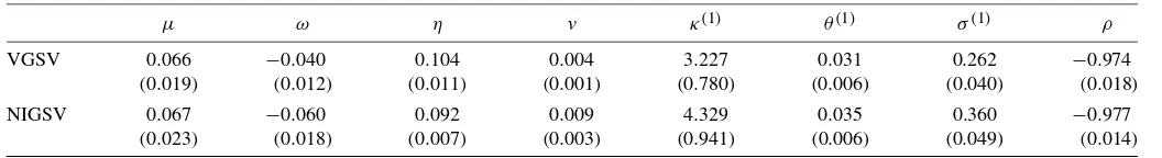
To investigate the performance of different filtering meth-ods in real data applications, I first obtain parameter estimates with MCMC methods using the stock price data alone. MCMC methods are particularly suitable in continuous-time financial models and result in consistent parameter estimates (Johannes and Polson2003). They have been shown to outperform many competing methods (Jacquier, Polson, and Rossi1994; Ander-sen, Chung, and Sorensen1999). The problem of the unavail-ability of the risk-premium parameters remains. Thus I assume that the parameters of the jump process and of the volatility process remain the same under the change of measure. Table3
presents parameter estimates of the VGSV and NIGSV models. With these parameter estimates, I then implement the filtering methods introduced previously.
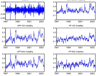
This two-step procedure allows one to to fully focus on ef-fects of filtering methods and avoids the efef-fects of parame-ter uncertainty. Because of their relevance to option pricing, only the volatility filtering results are provided here. Figure5
presents the filtered volatility using the S&P 500 index and
Table 3. Parameter estimates with MCMC methods
μ ω η v κ(1) θ(1) σ(1) ρ
VGSV 0.066 −0.040 0.104 0.004 3.227 0.031 0.262 −0.974
(0.019) (0.012) (0.011) (0.001) (0.780) (0.006) (0.040) (0.018)
NIGSV 0.067 −0.060 0.092 0.009 4.329 0.035 0.360 −0.977
(0.023) (0.018) (0.007) (0.003) (0.941) (0.006) (0.049) (0.014)
NOTE: MCMC methods are applied to estimate two models, which are discretized with a time intervalτ
yt=yt−τ+μτ+Xτ+ τVt(−1)τwt,
V(t1)=Vt(−τ1)+κ(1)θ(1)−Vt(−τ1)τ
+σ(1) τVt(−τ1)z(t1),
Xτ=ωSτ+η
Sτw˜t,
Sτ=gS(τ;1,v),
wheregSis the gamma process for the VG model and the inverse-Gaussian process for the NIG model. Both subordinators are constructed to have unit mean rate and variance ratev.
MCMC simulations are run with 50,000 total iterations and a burn-in period of 20,000.
Figure 5. Jointly filtered volatility. Filtering is implemented using the unscented sequential Monte Carlo method and the conventional method with the S&P 500 index and index options data for the VGSV and NIGSV models. The number of particles is 300 in the unscented method and 4000 in the conventional method. The online version of this figure is in color.
index options data for the VGSV and NIGSV models. The top panels present the index returns and the average Black– Scholes implied volatility, and the middle and lower panels present the filtered volatility using the proposed method (left panels) and the conventional method (right panels), respec-tively. Clearly, the filtered results using the proposed method are reasonably better than those obtained using the conventional method with comparison to the evolution of index returns and the Black–Scholes implied volatility. Even though the conven-tional method works acceptably in volatility filtering for the simulated data, it loses its ability for the real data. The pro-posed method is more robust than the conventional one for both the simulated data and the real data.
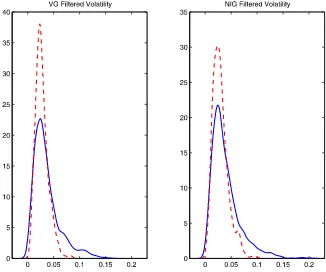
Figure 6 plots the kernel-smoothed density of the filtered volatility. The solid lines represent the densities of the filtered volatility from the proposed method, and the dashed lines are those from the conventional method. For both models, the den-sities from the conventional method have high peaks and short right tails. In contrast, the densities from the proposed un-scented method are more right-skewed and have longer right tails. These facts are consistent with the empirical observations and indicate that compared with the conventional method, the proposed method is more flexible for capturing different volatil-ity levels, especially the high volatilvolatil-ity during the financial cri-sis.
5.3 Option Pricing Implications
I now investigate option pricing implications. I divide the constructed near-the-money call options into nine groups with maturities of 10–45 days, 45–90 days, and 90–180 days and
with moneyness 0.94–0.97, 0.97–1.00, and 1.00–1.03. I then compute the absolute option pricing error using the filtered volatility obtained from the proposed and conventional meth-ods. The absolute option pricing error is defined as
Aerr= 1 N
T
t=1 nt
i=1
|Pimti −Pti|, (41)
whereN is the total number of options considered, T is the number of days, nt is the number of options at date t, and Pimti andPtiare the model-implied and market-observed option
prices of theith option at datet, respectively.
Table 4 presents ratios of the absolute option pricing er-rors. VGU/VGC (NIGU/NIGC) represents the ratio of option pricing errors of the VGSV (NIGSV) model using the filtered volatility obtained from the proposed method and the conven-tional method, and NIGU/VGU represents the ratio of the op-tion pricing errors of the NIGSV and VGSV models using the filtered volatility obtained from the proposed method. Clearly, all of the ratios of VGU/VGC and NIGU/NIGC are<1, indi-cating that the proposed method can capture the dynamics of the implied volatility surface much better than the conventional method can. The ratio of NIGU/VGU in each group is<1, im-plying that the NIGSV model performs better than the VGSV model in pricing options.
6. CONCLUDING REMARKS
In this article I have investigated time-changed infinite-activity derivatives pricing models from the sequential Bayesian perspective. I have proposed a sequential Monte Carlo method
Figure 6. Kernel-smoothed density of filtered volatility. The online version of this figure is in color.
with the proposal density generated by the unscented Kalman filter. This approach overcomes to a large extent the particle impoverishment problem inherent to the conventional particle filter and is more robust in real data applications. Effectively capturing the dynamics of states and disentangling the diffu-sion, stochastic volatility, and infinite activity jumps requires the use of both the underlying data and derivatives data. Simply taking the state transition law as the proposal density is inferior. One important issue I have not fully studied is parameter esti-mation. In this article I have assumed that the static parameters are known and are not taken into account in the analysis, but that parameters must be estimated. The particle filter-generated likelihood function is not a smoothed function of model pa-rameters because of the resampling step, and this irregularity
Table 4. Ratios of absolute option pricing errors
Moneyness (S/K)
Maturity Ratio 0.94–0.97 0.97–1.00 1.00–1.03
10–45 VGU/VGC 0.785 0.647 0.710 NIGU/NIGC 0.869 0.686 0.674 NIGU/VGU 0.939 0.873 0.733
45–90 VGU/VGC 0.770 0.786 0.792 NIGU/NIGC 0.771 0.733 0.738 NIGU/VGU 0.870 0.812 0.828
90–180 VGU/VGC 0.713 0.743 0.761 NIGU/NIGC 0.721 0.723 0.720 NIGU/VGU 0.804 0.791 0.754
NOTE: This table presents ratios of option pricing errors. VGU/VGC (NIGU/NIGC) represents the ratio of option pricing errors of the VGSV (NIGSV) model using the filtered volatility obtained from the proposed method and the conventional method. NIGU/VGU represents the ratio of the option pricing errors of the NIGSV model and the VGSV model using the filtered volatility obtained from the proposed method.
makes the usual gradient-based optimization routines difficult to apply. Pitt (2002) proposed a smooth resampling approach to overcome this problem. Unfortunately, this method works well only for one-dimensional state systems. For multidimensional systems, the proposed filtering method can be efficiently com-bined with the parameter estimation problem in the EM frame-work, in which the particle filter is only used to approximate the relevant expectations in the E-step, and the irregularity problem becomes immaterial in this setting because filtering and opti-mization are separated. Another potential approach is to com-bine particle filters with MCMC methods, as suggested by An-drieu, Doucet, and Holenstein (2010) and illustrated by Flury and Shephard (2008) using the conventional particle filter. Be-cause the proposed filtering method is more powerful than the conventional method, it can result in more accurate parameter estimates, especially the jump-related parameter estimates. This is important because the inability to capture the large jumps us-ing the conventional method might result in disastrous errors in derivative pricing and risk management, because these large jumps determine the tail behavior of the underlying distribu-tion and thus play a paramount role in pricing opdistribu-tions and risk management.
The batch estimation methods discussed above are time-consuming, however, especially when we consider the joint estimation using both the underlying data and the derivative data. Alternatively, parameters can be estimated sequentially as I have done for states. Online parameter estimation remains an open issue. Some methods have been proposed and applied by Liu and West (2001), Storvik (2002), Andrieu, Doucet, and Tadic (2005), and Johannes and Polson (2008), but each has some limitations. Thus, investigating this issue in the future for time-changed infinite-activity Lévy models would be of inter-est.
ACKNOWLEDGMENTS
I thank the editor, an associate editor, two anonymous ref-erees, Nick Polson, Andras Fulop, Carlo Favero, Fulvio Ortu, Pietro Muliere, and participants of the Bocconi University Finance Seminar, ESSEC Business School Finance Seminar, Manchester Business School Finance Seminar, the Fifth World Congress of Bachelier Finance Society, Sveriges Riksbank State-Space Modeling Workshop for Financial and Economic Time Series, Conference on Recent Developments in Finan-cial Econometrics, and X Workshop on Quantitative Finance for helpful comments.
[Received November 2008. Revised March 2010.]
REFERENCES
Andersen, T., Chung, H. J., and Sorensen, B. (1999), “Efficient Method of Mo-ments Estimation of a Stochastic Volatility Model: A Monte Carlo Study,” Journal of Econometrics, 91, 61–87. [477]
Andrieu, C., Doucet, A., and Holenstein, R. (2010), “Particle Markov Chain Monte Carlo,”Journal of the Royal Statistical Society, Ser. B, 72, 269–342. [479]
Andrieu, C., Doucet, A., and Tadic, V. B. (2005), “On-Line Parameter Estima-tion in General State-Space Models,” working paper, University of Bristol. [479]
Bakshi, G., Carr, P., and Wu, L. (2008), “Stochastic Risk Premiums, Stochastic Skewness in Currency Options and Stochastic Discount Factors in Interna-tional Economics,”Journal of Financial Economics, 87, 132–156. [470] Barndorff-Nielsen, O. E. (1998), “Processes of Normal Inverse Gaussian Type,”
Finance and Stochastics, 2, 41–68. [477]
Carr, P., and Madan, D. B. (1999), “Option Valuation Using the Fast Fourier Transform,”Journal of Computational Finance, 2, 61–73. [470]
Carr, P., and Wu, L. (2004), “Time-Changed Lévy Processes and Option Pric-ing,”Journal of Financial Economics, 71, 113–141. [470]
Carr, P., Geman, H., Madan, D. B., and Yor, M. (2003), “Stochastic Volatility for Lévy Processes,”Mathematical Finance, 13, 345–382. [469]
Chan, T. (1999), “Pricing Contingent Claims on Stocks Driven by Lévy Processes,”The Annals of Applied Probability, 9, 504–528. [470] Chourdakis, K. (2005), “Option Pricing Using the Fractional FFT,”Journal of
Computational Finance, 8, 1–18. [470]
Clark, P. K. (1973), “A Subordinated Stochastic Process Model With Fixed Variance for Speculative Prices,”Econometrica, 41, 135–156. [469] Cox, J. C., Ingersoll, J. E., and Ross, S. A. (1985), “A Theory of the Term
Structure of Interest Rates,”Econometrica, 53, 385–408. [469]
Doucet, A., de Freitas, N., and Gordon, N. (2001),Sequential Monte Carlo Methods in Practice, New York: Springer. [473]
Doucet, A., Godsill, S., and Andrieu, C. (2000), “On Sequential Monte Carlo Sampling Methods for Bayesian Filtering,”Statistics and Computing, 10, 197–208. [473]
Duffie, D., Pan, J., and Singleton, K. (2000), “Transform Analysis and Asset Pricing for Affine Jump-Diffusions,”Econometrica, 68, 1343–1376. [470]
Eraker, B., Johannes, M., and Polson, N. (2003), “The Impact of Jumps in Equity Index Volatility and Returns,”Journal of Finance, 58, 1269–1300. [471]
Flury, T., and Shephard, N. (2008), “Bayesian Inference Based Only on Simu-lated Likelihood: Particle Filter Analysis of Dynamic Economic Models,” technical report, Oxford University. [479]
Gerber, H. U., and Shiu, E. S. W. (1994), “Option Pricing by Esscher Trans-forms,”Transactions of Society of Actuaries, 46, 99–191. [470]
Gordon, N., Salmond, D., and Smith, A. (1993), “Novel Approach to Nonlinear and Non-Gaussian Bayesian State Estimation,”IEEE Proceedings F, 140, 107–113. [468,471]
Huang, J., and Wu, L. (2004), “Specification Analysis of Option Pricing Mod-els Based on Time-Changed Lévy Processes,”The Journal of Finance, 59, 1405–1439. [470]
Jacquier, E., Polson, N., and Rossi, P. (1994), “Bayesian Analysis of Stochastic Volatility Models,”Journal of Business & Economic Statistics, 12, 371– 389. [477]
Johannes, M., and Polson, N. (2003), “MCMC Methods for Continuous-Time Financial Econometrics,” inHandbook of Financial Econometrics, eds. L. P. Hansen and Y. Ait-Sahalia, Amsterdam: Elsevier. [477]
(2008), “Particle Filtering and Parameter Learning,” working paper, University of Chicago. [479]
Johannes, M., Polson, N., and Stroud, J. (2009), “Optimal Filtering of Jump-Diffusions: Extracting Latent States From Asset Prices,”Review of Finan-cial Studies, 22, 2559–2599. [468,469,471]
Julier, S. J., and Uhlmann, J. K. (1997), “A New Extension of the Kalman Fil-ter to Nonlinear Systems,” inProceedings of AeroSense: The 11th Interna-tional Symposium on Aerospace/Defense Sensing, Simulation and Controls, ed. I. Kadar, Orlando: SPIE, pp. 182–193. [469,471]
(2004), “Unscented Filtering and Nonlinear Estimation,”Proceedings of the IEEE, 92, 401–421. [469,471]
Li, J., Favero, C., and Ortu, F. (2009), “A Spectral Estimation of Tempered Stable Stochastic Volatility Models and Option Pricing,” working paper, ESSEC Business School. [470]
Liu, J., and Chen, R. (1998), “Sequential Monte Carlo Methods for Dynamic Systems,”Journal of the American Statistical Association, 93, 1032–1044. [473]
Liu, J., and West, M. (2001), “Combined Parameter and State Estimation in Simulation-Based Filtering,” inSequential Monte Carlo Methods in Prac-tice, eds. A. Doucet, N. de Freitas, and N. Gordon, New York: Springer. [479]
Madan, D., Carr, P., and Chang, E. (1998), “The Variance Gamma Process and Option Pricing,”European Finance Review, 2, 79–105. [473]
Michael, J., Schucany, W., and Haas, R. (1976), “Generating Random Variates Using Transformations With Multiple Roots,”The American Statistician, 30, 88–90. [477]
Pitt, M. (2002), “Smooth Particle Filters for Likelihood Evaluation and Maxi-mization,” working paper, University of Warwick. [479]
Pitt, M., and Shephard, N. (1999), “Filtering via Simulation: Auxiliary Particle Filters,”Journal of the American Statistical Association, 94, 590–599. [469] Storvik, G. (2002), “Particle Filters for State-Space Models With the Presence of Unknown Static Parameters,”IEEE Transactions on Signal Processing, 50, 281–289. [479]
Stroud, J., Muller, P., and Polson, N. (2003), “Nonlinear State-Space Models With State-Dependent Variances,”Journal of the American Statistical As-sociation, 98, 377–386. [468]
van der Merwe, R., de Freitas, J., Doucet, A., and Wan, E. (2000), “The Un-scented Particle Filter,” technical report, University of Cambridge. [469]