Full Terms & Conditions of access and use can be found at
http://www.tandfonline.com/action/journalInformation?journalCode=ubes20
Download by: [Universitas Maritim Raja Ali Haji] Date: 13 January 2016, At: 00:26
Journal of Business & Economic Statistics
ISSN: 0735-0015 (Print) 1537-2707 (Online) Journal homepage: http://www.tandfonline.com/loi/ubes20
Choice Behavior Under Time-Variant Quality
Klaus Moeltner & Jeffrey Englin
To cite this article: Klaus Moeltner & Jeffrey Englin (2004) Choice Behavior Under Time-Variant Quality, Journal of Business & Economic Statistics, 22:2, 214-224, DOI: 10.1198/073500104000000109
To link to this article: http://dx.doi.org/10.1198/073500104000000109
Published online: 01 Jan 2012.
Submit your article to this journal
Article views: 55
View related articles
Choice Behavior Under Time-Variant Quality:
State Dependence Versus “Play-It-by-Ear” in
Selecting Ski Resorts
Klaus M
OELTNERand Jeffrey E
NGLINDepartment of Resource Economics, University of Nevada, Reno, NV 89557 (moeltner@cabnr.unr.edu)
In past studies of consumer loyalty changes in brand attributes over time were generally unobservable and treated as additional model parameters. In this study we consider ski resorts, for which observable quality attributes change frequently. Using a repeated-purchase model with observed time-variant brand attributes, indicators for state dependence, and individual heterogeneity, we show that purchase history and time-variant site characteristics have a signicant and offsetting effect on repurchase decisions. This suggests a third category of consumer along with habit formers and variety seekers, the “play-it-by-ear” type, who, unaffected by purchase history, moves across brands in pursuit of high quality.
KEY WORDS: Random parameters; Repeated brand choice; Simulated choice probabilities; Time-variant quality features.
1. INTRODUCTION
When consumers repeatedly choose among several products, past choices can affect the probability of selecting a given prod-uct again at a later occasion. This phenomenon is commonly called “state dependence” (Heckman 1981a). Generally, state dependence can increase a consumer’s propensity to repur-chase a specic good (habit formation) or decrease the prob-ability of repurchase (variety-seeking). A key element of the research on the effects of state dependence to date has been the stability of observed characteristics for goods under con-sideration. The present study examines the role of purchase history for products with both xed and time-variant observed attributes. This allows us to disentangle effects attributable to state dependence from those associated with quality variation. Our empirical application is based on a set of ski areas in the Sierra Nevada; the time-variant quality attributes are snow and temperature.
In the marketing literature, state dependence is often called “purchase carryover” or “purchase-event feedback” (Allenby and Lenk 1995; Keane 1997). Understanding these forces that guide consumer choice is important to managers when making marketing and pricing decisions. Keane (1997) pointed out that temporary promotional efforts may affect consumer behavior well into the future if people are susceptible to habit formation. On the other hand, if consumer choice is relative insensitive to past purchases, or if variety-seeking is the dominant element of state dependence, then the promotional impact on sales may be short-lived.
The effect of state dependence on choice behavior has also become a topic of interest in the recreation literature (see, e.g., McConnell, Strand, and Bockstael 1990; Adamowicz 1994; Smith 1997). In those studies, the “products” from which peo-ple are choosing are not food or household items, as commonly investigated in marketing research, but rather recreation sites, such as shing spots (Adamowicz 1994; Swait, Adamovicz, and van Bueren 2000) or beach destinations (McConnell et al. 1990). In this context, understanding demand effects attribut-able to state dependence aid public land managers in making policy decisions on site access, pricing, and quality.
Regardless of the application, researchers must take care to disentangle “true” state dependence (Heckman 1981a) from the effect of time-variant exogenous variables and consumer heterogeneity. The estimated effect of true state dependence may be inated if consumer preferences are erroneously as-sumed to be homogeneous, or if time-variant exogenous vari-ables are omitted (Heckman 1981a; Keane 1997; Erdem and Sun 2001). In recent marketing contributions,heterogeneity has been explicitly captured in repeated-choice models by intro-ducing random coefcients into random utility models (RUMs) (Allenby and Lenk 1995; Erdem 1996; Keane 1997). Allenby and Lenk (1995), Erdem (1996), Keane (1997), and Erdem and Sun (2001) also included time-varying exogenousvariables (price and marketing effort) to disentangle their effect on pur-chase decisions from true state dependence.
Some marketing studies have also given consideration to the possibility that quality attributes of a given brand may change over time and/or may not be fully revealed to the con-sumer. Meyer (1982), Roberts and Urban (1988), and Erdem and Keane (1996) proposed brand choice models that capture perceived variability in product attributes over time. In the ap-proaches of Roberts and Urban (1988) and Erdem and Keane (1996), this uncertainty about quality from the consumer’s perspective is rooted in both incomplete information about a given product and in inherent product variability (i.e., uninten-tional changes in attributes due to aberrations in the production process). As agents gain more information through advertising, word of mouth, or direct consumption, they update their beliefs about the quality levels of each brand. This updating process, in turn, affects expected utility levels and choice probabilities. Meyer (1982) also allowed for incomplete information on prod-uct features, but added the possibility of weight shifts across attributes as consumers’ choice sets change during a sequential elimination process. In each of these studies, attribute variabil-ity is captured in form of stochastic model components, which
© 2004 American Statistical Association Journal of Business & Economic Statistics April 2004, Vol. 22, No. 2 DOI 10.1198/073500104000000109
214
are estimated together with the effects of exogenous choice factors.
The common element in these marketing contributionsis that from the researcher’s perspective, actual changes in attributes for a given brand over time are unobserved. For the household products generally considered in marketing applications, such as ketchup, peanut butter, and detergents, quality uctuations over time for a given brand are likely to be subtle and costly to measure. Recreation sites, on the other hand, can have pro-nounced changes in quality over time. Because these “brands” are not the end product of a highly controlled manufacturing process, they are by nature susceptible to a multitude of at-tribute changes over time. The importance of these changes for repeated site choices will depend on the type of recreational activity and on individual preferences. Ignoring the dynam-ics in site characteristdynam-ics when examining consumer loyalty or variety-seeking associated with a given recreational activity bears the risk of erroneous inferences about state dependence even when controlling for heterogeneity and marketing effects. This research extends existing marketing and recreation studies by analyzing the separate effects of observed quality changes and state dependence on consumer choice, while al-lowing for individual heterogeneity. In addition, we examine whether consumers who place a relatively large weight on a specic time and site-varying attribute are less likely to form habits. Conversely, we investigate if what appears to be be-havior driven by variety-seeking is in fact a manifestation of a “play-it-by-ear” attitude fueled by strong preferences for the changing attribute in question. This requires a product that is purchased relatively frequently and that exhibits both time-variant and time-intime-variant features. Ski resorts are well suited for this purpose. Their terrain and level of difculty remain un-changed over time, and on a given day the quality of a visit to the resort will be heavily affected by day-specic attributes, such as snow conditions and weather. Exploiting this natural experiment allows us to estimate a novel multichoice model with state dependence.
The remainder of this manuscript is structured as follows. In Section 2 we develop an econometric model of state depen-dence, observed time-variant quality effects, and heterogeneity. We then discuss the data and estimation results in Section 3, and operational implications for ski resort managers in Section 4. We provide concluding remarks and a summary of key ndings in Section 5.
2. MODEL FORMULATION
Following most brand choice studies, we embed our model in a RUM framework. Specically, we assume that the utility that individualiderives from a visit to resortjat timetis given by
UijtDD0j¢´iCA0j¢®iCPijt¢¯iCQ0jt¢°iCS0ijt¢±iC"ijt
DVijtC"ijt; iD1; : : : ;N; jD0; : : : ;J; tD1; : : : ;T;
(1)
whereDjis a vector of site-specic intercepts,Ajis a vector of
time-invariant resort attributes,Pijtis the price toifor visiting
resortjat time t,Qjt is a vector of quality characteristics that
change over resorts and time, andSijt is a vector of variables
associated with state dependence. The symbols´i,®i,¯i,°i,
and±i denote individual-specic coefcient vectors, and"ijt is
an iid random-error term.
Time periods are generally dened as purchase occasions in brand-choice studies (see, e.g., Allenby and Lenk 1995; Erdem 1996; Keane 1997). This preempts an investigation of inter-purchase time effects on choice decisions. As shown by Papatla and Krishnamurthi (1992), Chintagunta (1998), and Chintagunta and Prasad (1998), the time between purchases can affect the nature and intensity of state dependence. To cap-ture such effects in our model, and in synchronicity with the nature of our data (day trips), we choose days as the relevant time unit. It should be noted that for household goods, it is of-ten assumed that a given product is being consumed contin-uously throughout the interpurchase period (see, e.g., Papatla and Krishnamurthi 1992). This is different for recreation sites, where actual consumption ends with the visit. In fact, non-consumption at time t becomes a separate choice. This is usually modeled as the “staying-home” option or “nonpartic-ipation” in a RUM specication (e.g., Morey, Shaw, and Rowe 1991; Morey, Rowe, and Watson 1993). We follow Adamowicz (1994) by modeling nonparticipation as an additional alterna-tive to actual sites with associated utility
Ui0tD´i0CS0i0t¢±iC"i0t; (2)
where the “0” subscript indicates the stay-home option. We re-duce all quality indicators to a constant, and set the price to 0 for this choice. We do, however, retain variables measuring state dependence, as described later.
Although some studies on repeated choice let state depen-dence work through attributes of brands purchased in the past (e.g., Trivedi, Bass, and Rao 1994; Erdem 1996), we follow re-cent contributions in marketing (Keane 1997; Chintagunta and Prasad 1998; Erdem and Sun 2001) and recreation (Adamowicz 1994; Swait et al. 2000) by dening variables for state de-pendence based on brands (sites) chosen at previous purchase occasions.
The question then arises as to how far back into a con-sumer’s purchase history the model should reach. At one ex-treme, one could include only the choice decision made in the preceding period [i.e., the “rst-order” process (Erdem and Sun 2001) ]. At the other extreme, one could explicitly model the individual effect of all past choices made by the con-sumer (Heckman 1981b). Some authors have proposed a mid-dle ground by using a weighted average of past purchases to model choice history (Guadagni and Little 1983), or by includ-ing the number of uninterrupted times (i.e., “run”) a given brand was chosen before the current time period (Heckman 1981b; Bawa 1990). For our application, the number of time periods during the skiing season of interest (151 days) is far too large to allow the separate inclusion of all previous choices.
However, we a priori concur with McConnell et al. (1990) that recent visits should weigh more heavily for current site decisions than visits further in the past. We therefore include two indicators for past site choices in the model: the total num-ber of times that a given resort was chosen beforet.Nijt/, as in
Adamowicz (1994), and the consecutive number of times that a given resort was chosen up tot uninterrupted by any visits to other destinations (Rijt/. This variable conveys the notion of
“run” mentioned earlier. Because our data do not include many day-to-day runs, we allow for interruption by the stay-home op-tion for this indicator.
Our hypothesis is that whatever form of state dependence, if any, drives individualishould manifest itself more strongly through uninterruptedtripsRijtthan total trip countNijt. We also
specify two analogous indicators for the stay-home option: the number of times during the season before t that an individ-ual chose not to participate (Hit/(Adamowicz 1994), and the
number of consecutive days of nonskiing immediately preced-ing t.Dit/ (Provencher and Bishop 1997; Swait et al. 2000).
Thus the elements ofSijt,jD0; : : : ;J, materialize as resort. This implies thatRijtandDit equal 0 forjD0, whereas Hitapplies only to nonparticipation. SettingDit, the number of
days since the last ski trip, to 0 for the stay-home option pre-serves this indicator in a RUM specication. In essence,Ditcan
be interpreted as the relative effect of prolonged nonparticipa-tion on choice probabilities for resorts versus the probability to stay home in the current period as well.
Theoretically, both nonparticipation indicators could mea-sure a building up of “eagerness,” an increased probability of skiing as they grow large, or “rustiness,” the opposite effect. In essence, “eagerness” is the equivalent to “variety seeking” for actual sites, whereas “rustiness” corresponds to “habit for-mation” or “inertia.” Adamowicz (1994), for example, found that eagerness dominated behavior in his “rational model” (increased probability of visits as Hit increases), whereas
Provencher and Bishop (1997) found that as more time elapses since the last visit, the probability of participation decreases. Swait et al. (2000) reported initial rustiness following a preced-ing visit that turns into eagerness after about 10 weeks of non-participation. As we show, both eagerness and rustiness play a role in our model, with about 50% of riders adhering to each tendency.
As mentioned previously, to correctly estimate and interpret indicators for state dependence and the effect of time-variant exogenous factors, we need to control for individual hetero-geneity in our model. The rationale behind this requirement
is that probabilities associated with repeated choices made by the same person will be correlated due to unobserved individ-ual characteristics and preferences. If ignored, such inherent “tastes” may be incorrectly interpreted as an indication for state dependence. In recent contributions to the brand choice liter-ature, heterogeneous reactions to pricing and marketing vari-ables were found to be a signicant factor in the process that drives repeated-purchase decisions (Allenby and Lenk 1995; Erdem 1996; Keane 1997; Erdem and Sun 2001). Erdem (1996) and Erdem and Sun (2001) explicitly allowed for and found sig-nicant heterogeneity in how past brand choices and attributes affect individuals’ repurchase decisions.
In a RUM framework, it is convenient to introduce hetero-geneity through random coefcients (Revelt and Train 1998; McFadden and Train 2000). In contrast to Allenby and Lenk (1995) and Keane (1997), who allowed for time-varying taste parameters, and following Erdem (1996) and Erdem and Sun (2001), we assume that individual preferences remain constant throughout our research period. Collecting´i,®i,¯i,°i, and±i
into a single coefcient vector’i, we stipulate that parameters are distributed multivariate normal with
E.’i/D N’;
(4) E.’i¢’0i/D
Ȁ; iDj
0; i6Dj.
Thus we estimate a vector of parameter means, ’N, and the elements of the variance-covariance matrix Ä. In contrast to previous studies, the covariance terms in Ä are of major in-terest and importance in this article. Specically, we a priori expect a negative sign for covariances between (presumed posi-tive) coefcients associated with time-variant quality attributes and (positive) coefcients for state dependence, if habit for-mation dominates. Conversely, if a coefcient for state depen-dence is negative (indicating variety-seeking tendencies), its covariance with coefcients for time-variant quality should be positive. In other words, we hypothesize that the stronger the effect of quality seeking for a given individual, the smaller the absolute value of the coefcient for state dependence drawn for this individual.The intuition behind this premise is that quality-sensitive skiers (i.e., the play-it-by-ear types) should be less likely to be inuenced by past resort choices. As we show later, our results generally conrm this stipulation. This constitutes the key nding owing from this research.
We assume that remaining serial correlation in our model is accounted for by observed time-varying site attributes and indicators for state dependence. This implies that "ijt in (1)
is a truly random-error term uncorrelated with the elements of ’i. The stipulated density of this error will dictate the specication of choice probabilities. Two frequently used dis-tributions in the choice literature are normal, resulting in a mul-tivariate probit specication (Hausman and Wise 1978; Keane 1997), and type I extreme value. The latter distribution, in combination with the random coefcients in’i, yields a ran-dom parameter logit, or “mixed logit” model (Revelt and Train 1998; Brownstone and Train 1999). In either case, estimation of choice probabilities requires solving a high-dimensional in-tegral. As discussed by Layton (2000), the dimension of inte-gration proliferates with choice occasions in the multivariate
probit model, and with the number of random parameters in a mixed logit specication. In our application, each individual faces 1,359 choice occasions in a model with a limited number of random coefcients. For the sake of computational tractabil-ity, we therefore choose the mixed logit approach for our ap-plication. Thus the probability of skieri choosing optionjat timet, conditional on’i, is given by McFadden (1974)
Pijt.’i;’N;Ä/D
exp.Vijt.’i;’N;Ä// PJ
kD0exp.Vikt.’i;’N;Ä//
; (5)
whereVijt is dened as in (1). The conditional probability of
observing an individual’s entire sequence of trip decisions is therefore (Erdem 1996)
wheredijtis dened as in (3). Relaxing conditionality on
coef-cients yields
PiD Z
Ái
Pi.’i;’N;Ä/¢f.’i/d’i; (7)
wheref.’i/is the multivariate normal distribution. The dimen-sion of the integral in (7) is commensurate with the number of elements in’i. Because the evaluation of high-dimensional integrals is computationally impractical beyond an order of three or four given existing software capabilities, researchers have proposed simulation methods to estimate such probabil-ities and associated likelihood functions (Börsch-Supan and Hajivassiliou 1993; Keane 1994; McFadden and Train 2000). We follow the procedure outlined by Brownstone and Train (1999) by drawing a set of’ifromf.’i/, with some arbitrary starting values for’N andÄ. This allows us to compute (6) for all individuals. The process is repeatedR times, yielding the simulated choice probability (Erdem 1996; Layton 2000)
Q
where N denotes the number of individuals in the sample. The elements of’N andÄare updated throughout the optimiza-tion process and constitute the estimaoptimiza-tion output.
Aside from allowing for the examination and interpretation of potentially revealing covariance terms inÄ, our random pa-rameter specication provides two additional advantages. First, as discussed by Train (1998) and noted by Allenby and Lenk (1995), by introducing correlation across choice probabilities, we eliminate the problem of independenceof irrelevant alterna-tives that plagues standard conditional logit models. Second, as shown by Heckman (1981b), maximum likelihood procedures with random parameters will yield consistent estimates even under arbitrarily set initial conditions for state dependence, if N andT tend to innity. This is important in our application, because we do not have information on visits before the sam-pling period. Instead, we assume that all skiers start out with a “blank memory” and set the elements of Sijt to 0 for the
rst day of the season. Keane (1997) took a similar approach and showed robustness for his maximum likelihood estima-tors under xed initial conditions for a sample with large N (1,150 individuals) but rather smallT (about ve purchase oc-casions, on average). In our application, bothNandT are rea-sonably large (131 and 151), allowing us to invoke Heckman’s (1981b) nding as well.
3. EMPIRICAL ANALYSIS
3.1 Data
Our data stem from a spring 1998 survey of 131 randomly selected skiers and snowboarders (called “snow riders” here-inafter) at the University of Nevada, Reno. Each individual was asked to complete a chronology of trips to nine resorts in the Lake Tahoe area during the preceding 1997–1998 ski season. The exact time period spans 151 days from the end of November 1997 to the end of April 1998. All nine resorts were open during this period. Resort-specic infor-mation was collected from brochures and websites associ-ated with these ski areas. The source for our meteorologic data is the SNOTEL website established by the U.S. Depart-ment of Agriculture’s Natural Resources Conservation Service (www.wcc.nrcs.usda.gov/snotel). All seven SNOTEL sites con-sidered for this research are located in close vicinity of a given resort or pair of resorts.
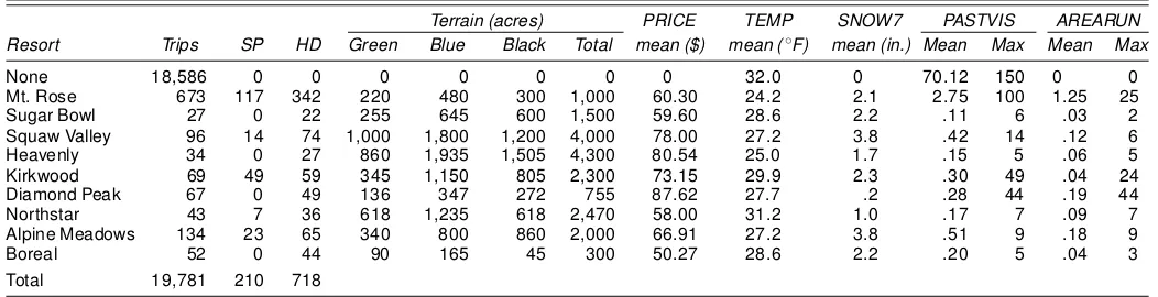
Table 1 summarizes the data and variables used in our -nal model specication. Overall, our dataset comprises 19,781
Table 1. Description of Data
Terrain (acres) PRICE TEMP SNOW7 PASTVIS AREARUN
Resort Trips SP HD Green Blue Black Total mean ($) mean (±F) mean (in.) Mean Max Mean Max
None 18,586 0 0 0 0 0 0 0 32.0 0 70.12 150 0 0 Mt. Rose 673 117 342 220 480 300 1,000 60.30 24.2 2.1 2.75 100 1.25 25 Sugar Bowl 27 0 22 255 645 600 1,500 59.60 28.6 2.2 .11 6 .03 2 Squaw Valley 96 14 74 1,000 1,800 1,200 4,000 78.00 27.2 3.8 .42 14 .12 6 Heavenly 34 0 27 860 1,935 1,505 4,300 80.54 25.0 1.7 .15 5 .06 5 Kirkwood 69 49 59 345 1,150 805 2,300 73.15 29.9 2.3 .30 49 .04 24 Diamond Peak 67 0 49 136 347 272 755 87.62 27.7 .2 .28 44 .19 44 Northstar 43 7 36 618 1,235 618 2,470 58.00 31.2 1.0 .17 7 .09 7 Alpine Meadows 134 23 65 340 800 860 2,000 66.91 27.2 3.8 .51 9 .18 9 Boreal 52 0 44 90 165 45 300 50.27 28.6 2.2 .20 5 .04 3 Total 19,781 210 718
choice occasions, including the stay-home option. Of these trips, 1,195 (6%) resulted in actual ski resort visits. As can be seen from the table, the lion’s share of actual trips (56%) were made to Mt. Rose, followed by Alpine Meadows (11%) and Squaw Valley (8%). Actual trips can be further divided into 210 visits (17.5%) by season pass (SP) holders, and 718 visits (60.1%) made on holidays (HD). The holiday dummy takes the value of 1 for designated university holidays and weekends and is set to 0 otherwise. It is also held at 0 for the stay-home option. The next four columns in Table 1 show the number of acres of beginner (green), intermediate (blue), and expert (black) terrain for a given resort, as well as the total size of the area. The variable PRICE includes round-trip travel costs from an individual’s ZIP code area to a given resort, plus ticket price for a specic resort, day, and individual. Although travel costs to and from a specic destination are assumed constant for a given rider during the research period, ticket prices vary by day of the week, time of season, gender, and age for some destinations. In addition, ticket prices are set to 0 for season pass holders. Our price variable reects these dynamic changes. The next two columns in Table 1 give time-varying quality variables. We hypothesizethat an individual’s riding experience will be strongly affected by weather and snow conditions on a given day. We use the average daily temperature in Fahrenheit (TEMP) to capture weather effects, and the cumulative water content of snowfall in inches (“pillow”) during the 7 days pre-ceding a given date to describe snow conditions. The resulting variable is labeled SNOW7 in the table. Data on actual snow volume were not available on a daily basis for our time period and sites. Because volume is a complex function of water con-tent, barometric pressure, temperature, and other unobserved meteorologic factors, we settle for pillow as a proxy for actual volume. Some additional aspects of snow quality will also be captured by the temperature variable. Specically, if snowfall has been abundant, then lower temperatures allow for better and longer lasting “powder” conditions. On the other hand, if little or no snow has recently been added to the overall pack, then low temperatures may result in hard and icy surfaces. The 7-day ac-cumulation period in SNOW7 provides for reasonable delays in skiers’ reaction to fresh snowfall while preserving a modicum of the “freshness” quality. As shown in the rst row of the table, TEMP and SNOW7 are arbitrarily set to 0 and 32 degrees for the nonparticipation option.
The remaining four columns in Table 1 show mean and max-imum values across sites for state-dependence variables Nijt
(PASTVIS) and Rijt (AREARUN) as dened in (3). The rst
row of PASTVIS corresponds to variableHit, the number of
days an individual had chosen not to ski throughout the sea-son before time t (termed PASTHOME hereinafter). As men-tioned earlier, AREARUN is set to 0 for the stay-home option. For actual sites, PASTVIS is largest for Mt. Rose for an aver-age visitor-day in our sample, with close to three earlier vis-its. Mt. Rose also had the highest maximum previous visits by a given snow rider (100), followed by Kirkwood (49) and Diamond Peak (44). In different order, these three resorts also lead in maxima foruninterruptedprevious visits (last column of Table 1).
The structure of our data results in 197,810 observations for the RUM framework outlined in Section 2. Our full specica-tion has 21 explanatory variables, including 9 intercept terms
for actual sites, SP, HD, PRICE, skill-adjusted terrain shares in natural log form (LNGREEN, LNBLUE, and LNBLACK), the climate variables TEMP and SNOW7, and the indicators for state dependencePASTVIS, PASTHOME, AREARUN, and DAYSHOME. Skill-adjusted terrain (SAT) is computed as total acres times the percent of terrain assigned to a specic skill cat-egory (greenDbeginner, blueDintermediate, blackDexpert) times the percentage of time during a season that an individ-ual uses any of the three categories. This concept is similar to Morey’s (1981) “effective physical characteristics.” However, in contrast to Morey, who implicitly assumed that a skier will use terrain appropriate for his skill level 100% of the time, we have the benet of actually knowing seasonal usage shares through direct elicitation.
All regressors are treated as random and are associated with a specic mean coefcient. To conserve on parameters, we estimate standard deviations for all regressors and a full variance-covariance matrix for the main variables of interest: time-variant quality attributes and state-dependence indicators PASTVIS, AREARUN, and DAYSHOME. This yields a to-tal of 52 model parameters for our unrestricted specication (model 1 in the next section).
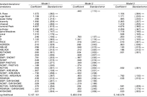
3.2 Estimation Results
Estimation results for coefcient means and the estimated el-ements ofÄ for three different specications are summarized in Tables 2 and 3. Model 1, our most general specication, in-cludes all regressors mentioned earlier plus resort intercepts. As discussed by Keane (1997), such intercepts may capture the effect of unobserved brand-specic features. In addition, it is likely that consumers’ preferences are heterogeneous with re-spect to these unobserved attributes as well. If this is the case, or if unobserved brand attributes are correlated with included regressors, then omission of brand intercepts will bias estima-tion results. Just as is the case if heterogeneity is ignored for ob-served regressors, the effect of state-dependenceindicators may be inated in the absence of such intercept terms. In our appli-cation, unobserved resort features could include the availability and quality of off-slope amenities (e.g., restaurants, lodges, shopping opportunities, day care for children), speed and com-fort of chair lifts, and so com-forth.
Model 2 omits site-specic terms and instead uses a non-participation intercept (D). Model 3 is identical to model 1 except for the omission of the time-variant quality indicators TEMP and SNOW7. For ease of interpretation,the variability of slope coefcients in Table 3 is given in terms of standard devi-ations, whereas their interdependence is shown in form of cor-relations. To be precise, maximum likelihood estimation pro-duces results forÄin form of its Cholesky factorization0(to impose the necessary constraints forÄ during optimization). For coefcients with covariances, the standard deviations and correlation terms reported in Table 3 are nonlinear functions of elements of0. Their reported sampling standard errors (values in parentheses in Table 3) are derived using the Delta method (e.g., Greene 1997).
The rst two columns in both tables show parameter esti-mates and standard errors for model 1. All coefcient means for site intercepts are highly signicant. The negative signs for all intercepts are expected, because these terms implicitly
Table 2. Estimation Results (parameter means)
Model 1 Model 2 Model 3
Parameters Coefcient Standard error Coefcient Standard error Coefcient Standard error
d 3.244 (.236) ***
Mt. Rose ¡3.263 (.333) *** ¡3.209 (.341) *** Sugar Bowl ¡7.343 (.458) *** ¡7.310 (.525) *** Squaw Valley ¡5.169 (.423) *** ¡5.026 (.416) *** Heavenly ¡6.823 (.542) *** ¡7.065 (.538) *** Kirkwood ¡7.148 (.538) *** ¡6.898 (.558) *** Diamond Peak ¡8.141 (.954) *** ¡8.204 (.732) *** Northstar ¡8.997 (.664) *** ¡8.232 (.589) *** Alpine Meadows ¡5.661 (.407) *** ¡5.547 (.433) *** Boreal ¡5.755 (.316) *** ¡5.570 (.325) *** SP .153 (.205) 1.288 (.238) *** .240 (.229) HD .750 (.095) *** .986 (.109) *** .697 (.100) *** PRICE ¡.055 (.004) *** ¡.047 (.004) *** ¡.052 (.004) *** LNGREEN .173 (.040) *** ¡.056 (.051) .204 (.046) *** LNBLUE ¡.007 (.035) ¡.237 (.046) *** ¡.046 (.032) LNBLACK .403 (.042) *** .225 (.038) *** .403 (.044) *** PASTHOME .004 (.005) ¡.038 (.005) *** .005 (.004) TEMP ¡.003 (.005) ¡.043 (.005) ***
SNOW7 .083 (.014) *** .072 (.013) ***
PASTVIS ¡.003 (.005) .046 (.005) *** ¡.004 (.004) AREARUN .032 (.014) ** .271 (.025) *** .042 (.012) *** DAYSHOME .003 (.003) .012 (.004) *** ¡.001 (.004) Log-likehood 5,107.101 5,650.518 5,140.579
NOTE: * signicant at the 10% level; ** signicant at the 5% level; *** signicant at the 1% level.
pare the probability of resort visitation with the probability of nonparticipation, the dominant choice in our dataset. In ad-dition, all estimated standard deviations for site dummies are signicant as well (Table 3), supporting the hypothesis of
pro-nounced consumer heterogeneity in preferences for unobserved resort features.
A similar result holds for HD. Although the effect of a hol-iday on the decision to visit a given resort is positive for the
Table 3. Estimation Results (parameter standard deviations and correlations)
Standard deviations/ correlations
Model 1 Model 2 Model 3
Coefcient Standard error Coefcient Standard error Coefcient Standard error
d .440 (.113) ***
Mt. Rose 1.072 (.082) *** 1.106 (.084) *** Sugar Bowl 1.108 (.213) *** 1.171 (.233) *** Squaw Valley .356 (.214) * .485 (.233) ** Heavenly 1.992 (.259) *** 2.265 (.257) *** Kirkwood 1.458 (.266) *** 1.418 (.255) *** Diamond Peak 4.607 (.615) *** 4.676 (.382) *** Northstar 2.496 (.291) *** 2.258 (.367) *** Alpine Meadows 1.142 (.147) *** 1.118 (.180) ***
Boreal 1.010 (.176) *** .928 (.165) ***
SP .246 (.106) ** .760 (.137) *** .250 (.135) * HD 1.122 (.083) *** 1.041 (.116) *** 1.210 (.102) *** PRICE .011 (.001) *** .016 (.001) *** .010 (.001) *** LNGREEN .010 (.029) .060 (.043) .063 (.036) * LNBLUE .056 (.018) *** .048 (.015) *** .120 (.015) *** LNBLACK .189 (.013) *** .212 (.020) *** .186 (.012) *** PASTHOME .000 (.001) .004 (.003) * .001 (.001) TEMP .004 (.006) .028 (.007) ***
TEMP / SNOW7 .781 (.203) *** ¡.997 (.030) *** SNOW7 .049 (.015) *** .048 (.016) *** TEMP /PASTVIS .208 (.271) .349 (.094) *** SNOW7 / PASTVIS ¡.189 (.330) ¡.274 (.354)
PASTVIS .004 (.001) *** .012 (.002) *** .002 (.001) TEMP / AREARUN ¡.907 (.108) *** .076 (.031) **
SNOW7 / AREARUN ¡.730 (.298) ** ¡.022 (.238)
PASTVIS / AREARUN .126 (.397) .403 (.153) *** ¡.762 (.132) *** AREARUN .035 (.012) *** .290 (.036) *** .035 (.012) *** TEMP / DAYSHOME .414 (.201) ** .239 (.159)
SNOW7 / DAYSHOME .029 (.338) ¡.219 (.189)
PASTVIS / DAYSHOME .372 (.294) .354 (.209) .581 (.209) *** AREARUN / DAYSHOME ¡.331 (.274) .202 (.245) ¡.641 (.174) *** DAYSHOME .021 (.004) *** .030 (.006) *** .023 (.003) *** Log-likelihood 5,107.101 5,650.518 5,140.579
NOTE: * signicant at the 10% level; ** signicant at the 5% level; *** signicant at the 1% level.
average participant (as indicated by the positive sign for the coefcient mean of HD in Table 2), there are individuals for whom this effect may well switch to a negative sign given the relatively high standard deviation for HD relative to its mean (Table 3). This is intuitively sound, because the occurrence of a holiday signies the relaxation of time constraints, but also implies increased crowdedness at most resorts.
The estimated effect of skill-adjusted terrain variables con-veys a preference for beginner runs (LNGREEN) and more difcult slopes (LNBLACK) for our sample of snow riders. This may indicate an acceleration effect in the acquisition of riding skills. Green areas are the only terrain accessible to novice skiers and boarders; thus, resorts with extensive acreage of beginner terrain will be preferred by this group for an ex-tended period. After this initiation period, riders advance to intermediate slopes. However, at this point the learning curve becomes much steeper, especially for the age group captured in our sample. This shortens the total riding time required to progress to advanced terrain. Once riders can access these areas, black terrain becomes a positive resort feature and remains de-sirable for an indenite time horizon. In other words, intermedi-ate slopes are sought out only during a relatively short transition period for this particular population of riders.
Of the time-varying quality attributes, only the mean coef-cient for snow is signicantly different from 0. Clearly, riders generally prefer more snow, but preferences are again heteroge-neous for this attribute, as indicated by the relatively large and signicant standard deviation for SNOW7 in Table 3. Speci-cally, for about 10%–20% of riders, recent snowfall has a neg-ative effect on visitation, applying our assumption of normality for random parameters (Erdem 1996). This may be related to difcult driving conditions during and immediately after winter storms.
The state-dependence indicators PASTVIS, PASTHOME, and DAYSHOME do not have a signicant mean effect on site choice in model 1. In contrast, the mean coefcient for AREARUN is highly signicant. Its positive sign indicates that the average rider exhibits habit-forming tendencies in the short run. However, the correspondingnontrivial and signicant stan-dard deviation for this indicator (Table 3) suggests the possibil-ity of variety-seekingfor about 20% of our population.It should be noted that although PASTVIS and DAYSHOME do not af-fect destination choices for the average rider, the signicant estimated standard deviations for these parameters (Table 3) indicate that they may affect site decisions for some individ-uals.This is especially true for the coefcient of DAYSHOME, which exhibits a standard deviation that is substantially larger than its estimated mean of 0. This in turn implies that about equal shares of riders are affected by eagerness and rustiness due to prolonged nonparticipation.
As can be seen in Table 3, model 1 also yields some sig-nicant correlation terms. In general, a sigsig-nicant correlation between two random coefcients associated with some ex-planatory variables would be indicative of an interactive effect of the two regressors on site choices. Given that both moments of the marginal distribution for the slope coefcient associated with temperature are estimated to be arbitrarily close to 0, the correlation terms for TEMP/SNOW7, TEMP/AREARUN, and
TEMP/DAYSHOME probably should not be given much im-portance. In contrast, the relatively large, negative, and signif-icant correlation term for SNOW7/AREARUN is as expected; riders who have relatively high (low) preferences for fresh snow are less (more) likely to be affected by visitation history, as measured by uninterrupted recent visits to a specic destina-tion. This key result supports our initial hypothesis that time-varying quality attributes and state dependencemay have a joint and potentially offsetting impact on repurchase decisions.
The mean parameter estimates associated with the second specication (model 2) are provided in the center columns of Table 2. The omission of site-specic intercept terms in this model has a strong effect on estimated parameters. Most no-tably, coefcients for all state-dependence indicators increase substantially and exhibit high statistical signicance. In light of the signicant means and standard deviations for site inter-cepts in model 1, the parameters generated by model 2 mani-fest the omitted variable problems discussed at the beginning of this section. Clearly, what is interpreted as “long-run habit forming” (PASTVIS, PASTHOME) and “short-run build-up of eagerness” (DAYSHOME) in model 2 appears to be primarily a reection of preferences for some unobserved resort-specic attributes for the representative rider. Thus model 2 is plagued by “spurious state dependence” (Heckman 1981a).
The omission of site intercepts also affects the coefcient means of SP and TEMP. Both are highly inated and estimated to be signicantly different from 0. For SP, this can be ex-plained by the fact that the vast majority of season passes are held for Mt. Rose and Alpine Meadows. In model 2, the ef-fect of having a season pass on choice probability is smeared across all destinations. Because Mt. Rose and Alpine Meadows are by far the most-visited sites for SP holders and nonholders alike, the coefcient for SP in model 1 likely captures the ef-fect of omitted quality attributes for these areas. With respect to TEMP, a possible explanation for this outcome is the fact that is the variability of average daily temperature is much less pronounced within and across resorts than is the variability in recent snowfall. Accordingly, the effect of TEMP is largely ab-sorbed by the site intercepts in model 1. Given the bias in the mean coefcients produced by model 2, the elements ofÄfor this model are equally awed. A discussion of these terms is thus omitted.
Our nal specication, model 3, reinstates site intercepts but omits the time-variant regressors TEMP and SNOW7. The resulting parameter estimates are shown in the last set of columns of Tables 2 and 3. They are similar to those gener-ated by model 1, with one noteworthy exception: the estimgener-ated mean coefcient for short-run state dependence (AREARUN) gains in both magnitude and signicance. This is yet another manifestation of Heckman’s (1981a) spurious state-dependence problem. In this case, the coefcient for AREARUN absorbs some of the effect of the omitted indicators for time-variant weather conditions.
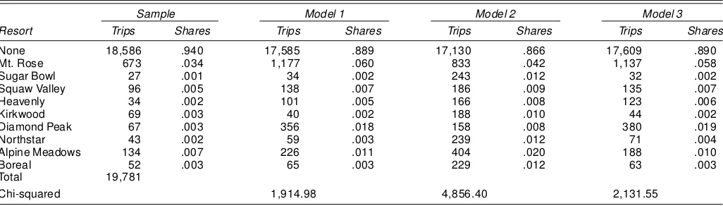
The inferiority of models 2 and 3 compared with model 1 is also highlighted by their much lower log-likelihood values. Corresponding likelihood ratio (LR) tests clearly reject the null hypotheses that brand intercepts and time-variant quality at-tributes have no effect on repeated site choices. It should be
Table 4. Seasonal Shares (including nonparticipation)
Sample Model 1 Model 2 Model 3
Resort Trips Shares Trips Shares Trips Shares Trips Shares
None 18,586 .940 17,585 .889 17,130 .866 17,609 .890 Mt. Rose 673 .034 1,177 .060 833 .042 1,137 .058 Sugar Bowl 27 .001 34 .002 243 .012 32 .002 Squaw Valley 96 .005 138 .007 186 .009 135 .007 Heavenly 34 .002 101 .005 166 .008 123 .006 Kirkwood 69 .003 40 .002 188 .010 44 .002 Diamond Peak 67 .003 356 .018 158 .008 380 .019 Northstar 43 .002 59 .003 239 .012 71 .004 Alpine Meadows 134 .007 226 .011 404 .020 188 .010
Boreal 52 .003 65 .003 229 .012 63 .003
Total 19,781
Chi-squared 1,914.98 4,856.40 2,131.55
noted that some parameters are restricted under the alterna-tive hypotheses (because variances cannot be negaalterna-tive). As dis-cussed by Barlow, Bremner, and Brunk (1972) and Chen and Cosslett (1998), the resulting LR statistics follow a mixed chi-squared distribution, and standard LR test results may be biased toward not rejecting the null hypothesis. In this application, the resulting LR values are well above the upper bound for the critical chi-squared(.05) value for such a mixed distribution. Thus, the adjustment procedure proposed by Chen and Cosslett (1998) would not affect our test results in this case.
4. SHARE PREDICTIONS AND
MARKETING SIMULATIONS
To compare the predictive power of our models, we fol-low Allenby and Lenk’s (1995) approach of estimating average choice probabilities over all individuals and choice occasions for all destinations. These aggregate choice shares for models 1, 2, and 3, together with actual sample shares, are presented in Tables 4 and 5. Table 4 captures all choices, including the non-participation option. Table 5 focuses on actual trips to ski areas. Because our models allow for random parameters, estimates are based on simulations using 1,000 different vectors of’O, drawn from the multivariate normal distribution with mean’ON
and variance-covariance matrixÄO. Approximations of trip g-ures corresponding to estimated shares are derived by multiply-ing shares by the total number of observed choice occasions (19,781 for Table 4 and 1,195 for Table 5). When nonparticipa-tion is included, all models generally overpredict trips to actual
resorts by varying degrees and slightly underpredict nonpartic-ipation choices. When only actual trips are considered, mod-els 1 and 3 predict trips to most resorts fairly well, whereas predictions generated by model 2 deviate more signicantly from sample results for most destinations. In the spirit of Keane (1997), the tables also include chi-squared statistics based on squared deviations between actual and predicted shares. As in-dicated by these values, the overall predictive power of model 1, our most general specication, is superior to that of models 2 and 3 with and without nonparticipation.
A resort manager may be interested in estimating the impact of promotional efforts and associated state-dependence effects on daily and seasonal market shares. Given that most actual trips were made to Mt. Rose ski area, and considering the good t of our estimated models for this destination (see Table 5), we focus on this resort for our marketing scenarios. Specically, we simulate six pricing scenarios. Scenarios 1 and 2 correspond to price reductions of $5 and $10, to all visitors for days 12–18 (Monday, December 8–Sunday, December 14). This time slot was chosen to leave ample time for state dependence to take effect throughout the remainder of the season. Also, actual vis-itation shares for Mt. Rose had reached standard levels by that week. Scenarios 3 and 4 simulate the same price reductions with extension through day 25. During the 1997–1998 ski sea-son, Mt. Rose offered two weekday specials that continued through the entire ski season: “Ladies Thursdays” (a $15 day pass for female visitors) and “Student Wednesdays” (a $10 day pass for students). Scenarios 5 and 6 investigate the impacts of “undoing” these promotions. Specically, scenario 5 imposes a
Table 5. Seasonal Shares (actual trips only)
Sample Model 1 Model 2 Model 3
Resort Trips Shares Trips Shares Trips Shares Trips Shares
Mt. Rose 673 .563 641 .536 376 .315 626 .524 Sugar Bowl 27 .023 18 .015 110 .092 17 .015 Squaw Valley 96 .080 75 .063 84 .070 74 .062
Heavenly 34 .028 55 .046 75 .063 67 .056
Kirkwood 69 .058 22 .018 85 .071 24 .020
Diamond Peak 67 .056 194 .162 71 .060 209 .175 Northstar 43 .036 32 .027 108 .090 39 .033 Alpine Meadows 134 .112 123 .103 182 .152 103 .087
Boreal 52 .044 36 .030 104 .087 35 .029
Total 1,195
Chi-squared 303.06 607.26 387.93
Table 6. Discount Scenarios
Scenario Time period Price change
1 Days 12–18 ¡$5
2 Days 12–18 ¡$10
3 Days 12–25 ¡$5
4 Days 12–25 ¡$10
5 Every Thursday C$23 6 Every Wednesday C$28
price increase of $23 to reach the standard day pass price of $38 for all skiers and boarders who had received a ladies’ discount. Similarly, scenario 6 increases day pass prices to student day beneciaries by $28. The pricing scenarios are summarized in Table 6. We implement these scenarios using model 1, our pre-ferred specication.
For each person, the simulations are conducted as follows. First, all exogenous price changes are incorporated into the data. Second, visitation probabilitiesPjt,jD0; : : : ;J, are
up-dated for the rst day of the scenario implementation (tDa). A choice or “hit” for day a is then simulated by dividing the unit interval intoJC1 segments corresponding in width toPja, jD0; : : : ;J, drawing a random term from the uniform.0;1/
distribution, noting the segment into which it falls, and match-ing the segment with the associated site. Conditionalon the out-come of this step, all state-dependencecounters forall sitesare then updated for the following day (tDaC1) according to the denitions in (3). Next, all choice probabilities for that day are adjusted to incorporate the updated state-dependence counters. A new site is drawn, state-dependence counters are updated fortDaC2, and so on, until the end of the research period (tDT). For each rider, this process is repeatedRD1,000 times. For each dayathroughT, simulated daily visitation shares are then determined by averaging updated daily probabilities over theRrepetitions and over all respondents. Finally, average sea-sonal shares for all sites are derived by averaging these aggre-gate daily shares over time periods. The resulting simulated shares are then compared with daily and seasonal shares gen-erated by model 1 using the original set of data. To conserve on computation time, this process is implemented using the mean vector of model coefcients,’N.
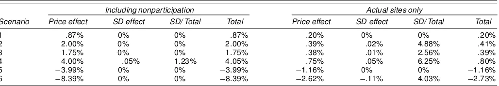
The aggregate seasonal effects for Mt. Rose and scenarios 1–6 are summarized in Table 7. The terms in the “total” column denote the time-averaged difference in daily shares between a given scenario and the baseline model. In essence, these val-ues can be interpreted as the percentage change in market shares relative to the baseline scenario on a typical day of the season. For simplicity, we assume that any change in daily shares ob-served on days of actual price changes are pure price effects
and changes in shares on other days are pure state-dependence effects. This allows for decomposition of total effect into an av-erage price effect and an avav-erage state-dependence effect for a typical season day. The left half of the table incorporates all choice options, including nonparticipation, whereas the right half considers scenario effects for actual resorts only.
As expected, the aggregate gain in daily shares increases with magnitude and length of the price promotion. Doubling the price discount (scenario 2) and doubling the duration of the discount period (scenario 3) have approximately equal effects on average share gains (2% and 1.75% with nonparticipation; .41% and .39% for actual sites only). Both promotions com-bined (scenario 4) approximately quadruple the initial share gain from scenario 1. Second, for all four scenarios, average state-dependence effects are arbitrarily close to 0. This is not surprising given that the only signicant state-dependenceindi-cator in model one is AREARUN, the counter for uninterrupted recent visits. This indicator, in turn is not likely to take on large values, because it is set to 0 every time a different actual site is chosen.
Generally, promotional gains relative to baseline shares ap-pear more pronounced when the nonparticipation option is in-cluded in the analysis compared with actual site–only results. This difference should be interpreted with caution, however, because the average daily baseline share for Mt. Rose is much smaller when nonparticipationis an included option than when only actual resorts are considered (1%–3% vs. 70%–80%). Thus, even an incremental increase in actual visits will translate into a much more pronounced percentage gain in the rst case. For the remaining scenarios, which eliminate existing weekly discounts for specic segments of riders, the table indicates that time-averaged share losses due to price effects are substantially higher under scenario 6 (students’ day,¡8:4%) than under sce-nario 5 (ladies’ day,¡4%). This result is not surprising, given that close to 90% of riders in our sample are students, compared with 43% of female participants.
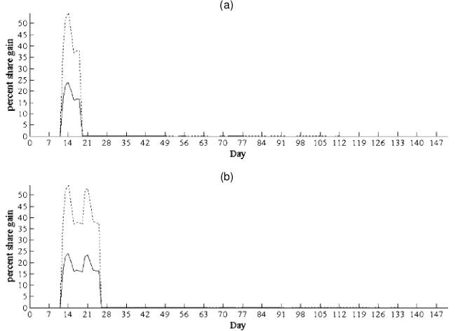
It should be noted that the share gains presented in Table 7 are “smeared” over the entire season, regardless of the actual days during which they take effect. Share gains for a specic day can be much more pronounced than the seasonal average. This can be seen in Figure 1, which shows the magnitude of daily share gains relative to the no-discount baseline for each day of the season for scenarios 1–4. The peaks of the time series indicate share gains through price effects, which can amount to more than 50% relative to the same time segment in the baseline sce-nario. As expected, daily gains increase with the magnitude of the price reduction (dotted lines vs. solid lines in the gure). The prolongation of a given discount approximately duplicates
Table 7. Average Daily Changes in Choice Shares
Including nonparticipation Actual sites only
Scenario Price effect SD effect SD/ Total Total Price effect SD effect SD/ Total Total
1 .87% 0% 0% .87% .20% 0% 0% .20%
2 2.00% 0% 0% 2.00% .39% .02% 4.88% .41%
3 1.75% 0% 0% 1.75% .38% .01% 2.56% .39%
4 4.00% .05% 1.23% 4.05% .75% .05% 6.25% .80% 5 ¡3.99% 0% 0% ¡3.99% ¡1.16% 0% 0% ¡1.16% 6 ¡8.39% 0% 0% ¡8.39% ¡2.62% ¡.11% 4.03% ¡2.73%
(a)
(b)
Figure 1. Daily Market Share Gains Due to Price Discounts (——, $5; - - - - -, $10) for (a) Days 12–18 and (b) Days 12–25. Price effects reach substantial magnitude during the promotion period, whereas state-dependence effects are arbitrarily close to 0 for these scenarios. Price effect peaks reect the additional impact of ladies’ day and students’ day discounts.
price effects for the rst period [Figs. 1(a) vs. 1(b)]. As for sea-sonal aggregates, state-dependence effects are not of measur-able magnitude in this day-by-day examination.
Figure 2 shows the impact of ladies’ day and students’ day discounts on daily share gains relative to scenarios 5 and 6, which eliminate these repeated weekly promotions. These daily gains are clearly associated with the days of promotion (Thurs-days for ladies’ day, Wednes(Thurs-days for students’ day), and remain relatively constant in magnitude over the season. Share gains
are approximately twice as high for the students’ day promo-tion than for the ladies’ day scenario (60% vs. 30%).
5. CONCLUSION
Repeated consumer choices over substitute products can induce habit formation or variety-seeking. These tendencies, when recognized, aid managers in marketing and pricing deci-sions. Traditional consumer goods, such as detergents and soft
(a)
(b)
Figure 2. The Daily Share Gains Due to Price Effects of Repeated Weekly Discounts: (a) Ladies’ Day; (b) Students’ Day. These gains remain relatively constant in magnitude over the season; they are more pronounced for the students’ day scenario.
drinks, generally exhibit constant quality over a given research period. For such products, the main analytical and economet-ric challenge when investigating the forces of state dependence is to distinguish between true effects of past purchases and in-dividual heterogeneity. In this article we have considered con-sumer goods for which quality attributes change frequently over time. Ski areas serve as a good example of such a commod-ity, because daily snow and weather conditions strongly affect the level of resort benets owing to visitors. To disentangle the impact of quality changes, state dependence, and consumer preferences on destination choice, we have proposed a model that explicitly includes time-varying quality features as well as indicators for state dependence, while allowing for individual heterogeneity.
A key result that ows from our analysis is that time-variant quality attributes can have a signicant impact on consumer choice. Omitting these characteristics leads to biased coef-cients for state dependence. The same problem occurs if time-invariant site characteristics are excluded from the model. These effects are illustrated by comparing three different model specications for repeated site choice. Generally, state depen-dence diminishes, but remains a signicant force in a correctly specied model. The lion’s share of this effect is linked to recent purchase history. In our application, habit formation clearly dominates variety-seeking. Most importantly, our results in-dicate that time-variant quality and habit formation can have an offsetting effect on consumer choice. Specically, we nd evidence that visitors to whom quality matters more are less likely to exhibit habitual behavior. This suggests that along with habit formers and variety-seekers, there exists a third cat-egory of consumer in repeated-choice settings: the play-it-by-ear type, who, relatively unaffected by purchase history, will move across brands in pursuit of high quality. Identifying these quality-seekers and analyzing how their reactions to pricing and marketing strategies differ from those exhibited by the tradi-tional state-dependence types is a subject for future research.
ACKNOWLEDGMENTS
The authors thank J. Scott Shonkwiler and Roger von Haefen for helpful suggestions and comments. This research was sup-ported in part by the Nevada Agricultural Experiment Station, publication #51031316.
[Received December 2001. Revised July 2003.]
REFERENCES
Adamowicz, W. L. (1994), “Habit Formation and Variety Seeking in a Discrete Choice Model of Recreation Demand,”Journal of Agriculture and Resource Economics, 19, 19–31.
Allenby, G. M., and Lenk, P. J. (1995), “Reassessing Brand Loyalty, Price Sen-sitivity, and Merchandising Effects on Consumer Brand Choice,”Journal of Business & Economic Statistics, 13, 281–289.
Barlow, R. E., Bremner, J. M., and Brunk, H. D. (1972),Statistical Inference Under Order Restrictions, New York: Wiley.
Bawa, K. (1990), “Modeling Inertia and Variety Seeking Tendencies in Brand Choice Behavior,”Marketing Science, 9, 263–278.
Börsch-Supan, A., and Hajivassiliou, V. A. (1993), “Smooth Unbiased Multi-variate Probability Simulators for Maximum Likelihood Estimation of Lim-ited Dependent Variable Models,”Journal of Econometrics, 58, 347–368. Brownstone, D., and Train, K. (1999), “Forecasting New Product Penetration
With Flexible Substitution Patterns,”Journal of Econometrics, 89, 109–129.
Chen, H. Z., and Cosslett, S. R. (1998), “Environmental Quality Preference and Benet Estimation in Multinomial Probit Models: A Simulation Approach,”
American Journal of Agricultural Economics, 80, 512–520.
Chintagunta, P. K. (1998), “Inertia and Variety Seeking in a Model of Brand-Purchase Timing,”Marketing Science, 17, 253–270.
Chintagunta, P. K., and Prasad, A. R. (1998), “An Empirical Investigation of the (Dynamic McFadden) Model of Purchase Timing and Brand Choice: Im-plications for Market Structure,”Journal of Business & Economic Statistics, 16, 2–12.
Erdem, T. (1996), “A Dynamic Analysis of Market Structure Based on Panel Data,”Marketing Science, 15, 359–378.
Erdem, T., and Keane, M. P. (1996), “Decision-Making Under Uncertainty: Capturing Dynamic Brand Choice Processes in Turbulent Consumer Goods Markets,”Marketing Science, 15, 1–20.
Erdem, T., and Sun, B. (2001), “Testing for Choice Dynamics in Panel Data,”
Journal of Business & Economic Statistics, 19, 142–152.
Greene, W. H. (1997), Econometric Analysis, Upper Saddle River, NJ: Prentice-Hall.
Guadagni, P., and Little, J. (1983), “A Logit Model of Brand Choice Calibrated on Scanner Data,”Marketing Science, 2, 203–238.
Hausman, J. A., and Wise, D. A. (1978), “A Conditional Probit Model for Qual-itative Choice: Discrete Decisions Recognizing Interdependence and Hetero-geneous Preferences,”Econometrica, 46, 403–426.
Heckman, J. J. (1981a), ”Heterogeneity and State Dependence,” in Stud-ies in Labor Markets, ed. S. Rosen, Chicago: Chicago University Press, pp. 91–139.
(1981b), “The Incidental Parameter Problem and the Problem of Initial Conditions in Estimating a Discrete Time-Discrete Data Stochastic Process,” inStructural Analysis of Discrete Data With Econometric Applications, eds. C. F. Manski and D. McFadden, Cambridge, MA: MIT Press, pp. 114–178. Keane, M. P. (1994), “A Computationally Practical Simulation Estimator for
Panel Data,”Econometrica, 62, 95–116.
(1997), “Modeling Heterogeneity and State Dependence in Consumer Choice Behavior,”Journal of Business & Economic Statistics, 15, 310–327. Layton, D. F. (2000), “Random Coefcient Models for Stated Preference
Sur-veys,”Journal of Environmental Economics and Management, 40, 21–36. McConnell, K., Strand, I. E., and Bockstael, N. E. (1990), “Habit Formation
and the Demand for Recreation: Issues and a Case Study,” inAdvances in Applied Micro Economics, eds. A. N. Link and V. K. Smith, Greenwich, CT: JAI Press, pp. 217–235.
McFadden, D. (1974), ”Conditional Logit Analysis of Qualitative Choice Be-havior,” inFrontiers in Econometrics, ed. P. Zarembka, New York: Academic Press, pp. 105–142.
McFadden, D., and Train, K. (2000), “Mixed MNL Models for Discrete Re-sponses,”Journal of Applied Econometrics, 15, 447–470.
Meyer, R. J. (1982), “A Descriptive Model of Consumer Information Search Behavior,”Marketing Science, 1, 93–121.
Morey, E. R. (1981), “The Demand for Site-Specic Recreational Activi-ties: A Characteristics Approach,”Journal of Environmental Economics and Management, 8, 345–371.
Morey, E. R., Rowe, R. D., and Watson, M. (1993), “A Repeated Nested-Logit Model of Atlantic Salmon Fishing,”American Journal of Agricultural Eco-nomics, 75, 578–592.
Morey, E. R., Shaw, W. D., and Rowe, R. D. (1991), “A Discrete-Choice Model of Recreational Participation, Site-Choice, and Activity Valuation When Complete Trip Data Are Not Available,”Journal of Environmental Economics and Management, 20, 181–201.
Papatla, P., and Krishnamurthi, L. (1992), “A Probit Model of Choice Dynam-ics,”Marketing Science, 11, 189–206.
Provencher, B., and Bishop, R. C. (1997), “An Estimable Dynamic Model of Recreation Behavior With an Application to Great Lakes Angling,”Journal of Environmental Economics and Management, 33, 107–127.
Revelt, D., and Train, K. (1998), “Mixed Logit With Repeated Choices: House-holds’ Choices of Appliance Efciency Level,”Review of Economics and Statistics, 80, 647–657.
Roberts, J. H., and Urban, G. L. (1988), “Modeling Multiattribute Utility, Risk, and Belief Dynamics for New Consumer Durable Brand Choice,” Manage-ment Science, 34, 167–185.
Smith, V. K. (1997), “Time and the Valuation of Environmental Resources,” Washington, DC: Resources for the Future.
Swait, J., Adamovicz, W., and van Bueren, M. (2000), “Choice and Tempo-ral Welfare Impacts: Dynamic GEV Discrete Choice Models,” staff paper, University of Alberta, Dept. of Rural Economy.
Train, K. (1998), “Recreation Demand Models With Taste Differences Over People,”Land Economics, 74, 230–239.
Trivedi, M., Bass, F. M., and Rao, R. C. (1994), “A Model of Stochastic Variety Seeking,”Marketing Science, 13, 274–297.