Full Terms & Conditions of access and use can be found at
http://www.tandfonline.com/action/journalInformation?journalCode=ubes20
Download by: [Universitas Maritim Raja Ali Haji] Date: 11 January 2016, At: 23:06
Journal of Business & Economic Statistics
ISSN: 0735-0015 (Print) 1537-2707 (Online) Journal homepage: http://www.tandfonline.com/loi/ubes20
Dynamic Censored Regression and the Open
Market Desk Reaction Function
de Robert Jong & Ana María Herrera
To cite this article: de Robert Jong & Ana María Herrera (2011) Dynamic Censored Regression and the Open Market Desk Reaction Function, Journal of Business & Economic Statistics, 29:2, 228-237, DOI: 10.1198/jbes.2010.07181
To link to this article: http://dx.doi.org/10.1198/jbes.2010.07181
View supplementary material
Published online: 01 Jan 2012.
Submit your article to this journal
Article views: 131
Supplementary materials for this article are available online. Please click the JBES link athttp://pubs.amstat.org.
Dynamic Censored Regression and the Open
Market Desk Reaction Function
Robert
DEJ
ONGDepartment of Economics, Ohio State University, 429 Arps Hall, Columbus, OH 43210 (dejong@econ.ohio-state.edu)
Ana María H
ERRERADepartment of Economics, Wayne State University, 656 W Kirby, 2095 FAB, Detroit, MI 48202 (amherrera@wayne.edu)
The censored regression model and the Tobit model are standard tools in econometrics. This paper pro-vides a formal asymptotic theory for dynamic time series censored regression when lags of the dependent variable have been included among the regressors. The central analytical challenge is to prove that the dynamic censored regression model satisfies stationarity and weak dependence properties if a condition on the lag polynomial holds. We show the formal asymptotic correctness of conditional maximum like-lihood estimation of the dynamic Tobit model, and the correctness of Powell’s least absolute deviations procedure for the estimation of the dynamic censored regression model. The paper is concluded with an application of the dynamic censored regression methodology to temporary purchases of the Open Market Desk. This article has supplementary material online.
KEY WORDS: Announcement effect; Censored regression; CLAD; Open market operations; Tobit.
1. INTRODUCTION
The censored regression model and the Tobit model are stan-dard tools in econometrics. In a time series framework, cen-sored variables arise when the dynamic optimization behavior of a firm or individual leads to a corner response for a signifi-cant proportion of time. In addition, right-censoring may arise due to truncation choices made by the analysts in the process of collecting the data (i.e., top coding). Censored regression mod-els apply to variables that are left-censored at zero, such as the level of open market operations or foreign exchange interven-tion carried out by a central bank, and in the presence of an in-tercept in the specification they also apply to time series that are censored at a nonzero point, such as the clearing price in com-modity markets where the government imposes price floors, the quantity of imports and exports of goods subject to quotas, and numerous other series.
The asymptotic theory for the Tobit model in cross-section situations has long been understood; see, for example, the treat-ment in Amemiya (1973). In recent years, asymptotic theory for the dynamic Tobit model in a panel data setting has been established using large-N asymptotics; see Arellano and Hon-oré (1998) and Honoré and Hu (2004). However, there is no result in the literature that shows stationarity properties of the dynamic censored regression model, leaving the application of cross-section techniques for estimating the dynamic censored regression model in a time series setting formally unjustified. This paper seeks to fill this gap. After all, a justication of stan-dard inference in dynamic nonlinear models requires laws of large numbers and a central limit theorem to hold. Such results require weak dependence and stationarity properties.
While in the case of linear AR models it is well known that we need the roots of the lag polynomial to lie outside the unit circle in order to have stationarity; no such result is known for nonlinear dynamic models in general and the dynamic regres-sion model in particular. The primary analytical issue addressed
in this paper is to show that under some conditions, the dynamic censored regression model as defined below satisfies stationar-ity and weak dependence properties. This proof is therefore an analogue to well-known proofs of stationarity of ARMA mod-els under conditions on the roots of the AR lag polynomial. The dynamic censored regression model under consideration is
yt=max
0, p
i=1
ρiyt−i+γ′xt+εt
, (1)
wherext denotes the regressor,εt is a regression error, we as-sume that γ ∈Rq, and we define σ2=Eεt2. One feature of the treatment of the censored regression model in this paper is thatεtis itself allowed to be a linear process [i.e., an MA(∞) process driven by an iid vector of disturbances], which means it displays weak dependence and is possibly correlated. While stationarity results for general nonlinear models have been de-rived in, for example, Meyn and Tweedie (1994), there appear to be no results for the case where innovations are not iid (i.e., weakly dependent or heterogeneously distributed). The reason for this is that the derivation of results such as those of Meyn and Tweedie (1994) depends on a Markov chain argument, and this line of reasoning appears to break down when the iid as-sumption is dropped. This means that in the current setting, Markov chain techniques cannot be used for the derivation of stationarity properties, which complicates our analysis substan-tially, but also puts our analysis on a similar level of generality as can be achieved for the linear model.
A second feature is that no assumption is made on the lag polynomial other than thatρmax(z)=1−ip=1max(0, ρi)zihas
© 2011American Statistical Association Journal of Business & Economic Statistics
April 2011, Vol. 29, No. 2 DOI:10.1198/jbes.2010.07181
228
its roots outside the unit circle. Therefore, in terms of the con-ditions onρmax(z)and the dependence allowed forεt, the aim
of this paper is to analyze the dynamic Tobit model on a level of generality that is comparable to the level of generality under which results for the linear AR(p) model can be derived. Note that intuitively, negative values forρjcan never be problematic when considering the stationarity properties of yt, since they “pullyt back to zero.” This intuition is formalized by the fact that only max(0, ρj)shows up in our stationarity requirement.
An alternative formulation for the dynamic censored regres-sion model could be
yt=y∗tI(y
∗
t >0), whereρ(B)y
∗
t =γ
′x
t+εt, (2) whereBdenotes the backward operator. This model will not be considered in this paper, and its fading memory properties are straightforward to derive. The formulation considered in this paper appears the appropriate one if the 0 values in the dynamic Tobit are not caused by a measurement issue, but have a genuine interpretation. In the case of a model for the difference between the price of an agricultural commodity and its government-instituted price floor, we may expect economic agents to re-act to the re-actually observed price in the previous period rather than the latent market clearing price, and the model considered in this paper appears more appropriate. However, if our aim is to predict tomorrow’s temperature from today’s temperature as measured by a lemonade-filled thermometer that freezes at 0◦ Celsius, we should expect that the alternative formulation of the dynamic censored regression model of Equation (2) is more appropriate.
The literature on the dynamic Tobit model appears to mainly consist of (i) theoretical results and applications in panel data settings, and (ii) applications of the dynamic Tobit model in a time series setting without providing a formal asymptotic the-ory. Three noteworthy contributions to the literature on dynamic Tobit models are Honoré and Hu (2004), Lee (1999), and Wei (1999). Honoré and Hu (2004) considers dynamic Tobit models and deals with the problem of the endogeneity of lagged values of the dependent variable in panel data setting, where the er-rors are iid,Tis fixed, and large-Nasymptotics are considered. In fact, the asymptotic justification for panel data Tobit models is always through a large-Ntype argument, which distinguishes this work from the treatment of this paper. For a treatment of the dynamic Tobit model in a panel setting, the reader is referred to Arellano and Honoré (1998, section 8.2).
Lee (1999) and Wei (1999) deal with dynamic Tobit models where lags of the latent variable are included as regressors. Lee (1999) considers likelihood simulation for dynamic Tobit mod-els with ARCH disturbances in a time series setting. The central issue in this paper is the simulation of the log likelihood in the case where lags of the latent variable (in contrast to the ob-served lags of the dependent variable) have been included. Wei (1999) considers dynamic Tobit models in a Bayesian frame-work. The main contribution of this paper is the development of a sampling scheme for the conditional posterior distributions of the censored data, so as to enable estimation using the Gibbs sampler with a data augmentation algorithm.
In related work, de Jong and Woutersen (2010) consider the dynamic time series binary choice model and derive the weak dependence properties of this model. This paper also considers
a formal large-Tasymptotic theory when lags of the dependent variable are included as regressors. Both this paper and de Jong and Woutersen (2010) allow the error distribution to be weakly dependent. The proof in de Jong and Woutersen (2010) estab-lishes a contraction mapping type result for the dynamic binary choice model; however, the proof in this paper is completely different, since other analytical issues arise in the censored re-gression context.
As we mentioned above, a significant body of literature on the dynamic Tobit model consists of applications in a time se-ries setting without providing a formal asymptotic theory. In-ference in these papers is either conducted in a classical frame-work, by assuming the maximum likelihood estimates are as-ymptotically normal, or by employing Bayesian inference. Pa-pers that estimate censored regression models in time series cover diverse topics. In the financial literature, prices subject to price limits imposed in stock markets, commodity future exchanges, and foreign exchange futures markets have been treated as censored variables. Kodres (1988,1993) uses a cen-sored regression model to test the unbiasedness hypothesis in the foreign exchange futures markets. Wei (2002) proposes a censored-GARCH model to study the return process of assets with price limits, and applies the proposed Bayesian estimation technique to Treasury bill futures.
Censored data are also common in commodity markets where the government has historically intervened to support prices or to impose quotas. An example is provided by Chavas and Kim (2006) who use a dynamic Tobit model to analyze the determinants of U.S. butter prices with particular attention to the effects of market liberalization via reductions in floor prices. Zangari and Tsurumi (1996) and Wei (1999) use a Bayesian ap-proach to analyze the demand for Japanese exports of passen-ger cars to the U.S., which were subject to quotas negotiated between the U.S. and Japan after the oil crisis of the 1970s.
Applications in time series macroeconomics comprise deter-minants of open market operations and foreign exchange inter-vention. Dynamic Tobit models have been used by Demiralp and Jordà (2002) to study the determinants of the daily transac-tions conducted by the Open Market Desk, and Kim and Sheen (2002) and Frenkel, Pierdzioch, and Stadtmann (2003) to esti-mate the intervention reaction function for the Reserve Bank of Australia and the Bank of Japan, respectively.
The structure of this paper is as follows. Section2presents our weak dependence results for(yt,xt)in the censored regres-sion model. In Section3, we show the asymptotic validity of the dynamic Tobit procedure. Powell’s (1984) LAD estimation procedure for the censored regression model, which does not assume normality of errors, is considered in Section 4. Sec-tion 5studies the determinants of temporary purchases of the Open Market Desk. Section6concludes.
2. MAIN RESULTS
We will prove that yt as defined by the dynamic censored regression model satisfies a weak dependence concept called
Lr-near epoch dependence. Near epoch dependence of random variablesyton a base process of random variablesηtis defined as follows:
230 Journal of Business & Economic Statistics, April 2011
Definition 1. Random variablesyt are calledLr-near epoch
dependent onηtif sup
t∈Z
E|yt−E(yt|ηt−M, ηt−M+1, . . . , ηt+M)|r
=ν(M)r→0 asM→ ∞. (3) The base process ηt needs to satisfy a condition such as strong or uniform mixing or independence in order for the near epoch dependence concept to be useful. For the definitions of strong (α-) and uniform (φ-) mixing see, for example, Gallant and White (1988, p. 23) or Pötscher and Prucha (1997, p. 46). The near epoch dependence condition then functions as a de-vice that allows approximation of yt by a function of finitely many mixing or independent random variablesηt.
For studying the weak dependence properties of the dynamic censored regression model, assume thatytis generated as
yt=max pendence results for the general dynamic censored regression model that contains regressors.
When postulating the above model, we need to resolve the question as to whether there exists a strictly stationary solution to it and whether that solution is unique in some sense. See, for example, Bougerol and Picard (1992) for such an analysis in a linear multivariate setting. In the linear modelyt=ρyt−1+ηt,
these issues correspond to showing that∞j=0ρjηt−jis a strictly stationary solution to the model that is unique in the sense that no other function of(ηt, ηt−1, . . .)will form a strictly stationary
solution to the model.
An alternative way of proceeding to justify inference could be by considering arbitrary initial values (y1, . . . ,yp) for the process instead of starting values drawn from the stationary dis-tribution, but such an approach will be substantially more com-plicated.
The idea of the strict stationarity proof of this paper is to show that by writing the dynamic censored regression model as a function of the laggedyt that are sufficiently remote in the past, we obtain an arbitrarily accurate approximation ofyt. Let
Bdenote the backward operator, and define the lag polynomial ρmax(B)=1−pi=1max(0, ρi)Bi. The central result of this pa-per, the formal result showing the existence of a unique back-ward looking strictly stationary solution that satisfies a weak de-pendence property for the dynamic censored regression model is now the following:
Theorem 1. If the linear processηtsatisfiesηt=∞i=0aiut−i,
wherea0>0,utis a sequence of iid random variables with den-sityfu(·),E|ut|r<∞for somer≥2,
its roots outside the unit circle, and for allx∈R,
P(ut≤x)≥F(x) >0 (5) c2, then the near epoch dependence sequence ν(M) satisfies ν(M)≤c1exp(−c2M1/3)for positive constantsc1andc2.
Our proof is based on the probability ofyt reaching 0 given the lastp values ofηt always being positive. This property is the key towards our proof and is established using the linear process assumption in combination with the condition of Equa-tion (5). Note that by the results of Davidson (1994, p. 219), our assumption onηtimplies thatηtis also strong mixing with α(m)=O(∞t=m+1G1t/(1+r)). Also note that for the dynamic Tobit model where errors are iid normal and regressors are ab-sent, the condition of the above theorem simplifies to the as-sumption thatρmax(z)has all its roots outside the unit circle.
One interesting aspect of the condition onρmax(z)is that
neg-ativeρiare not affecting the strict stationarity of the model. The intuition is that becauseyt≥0 a.s., negativeρican only “pullyt back to zero” and because the model has the trivial lower bound of 0 foryt, unlike the linear model, this model does not have the potential forytto tend to minus infinity.
3. THE DYNAMIC TOBIT MODEL
Defineβ =(ρ′, γ′, σ )′, whereρ=(ρ1, . . . , ρp), and define
b=(r′,c′,s)′ wherer is a (p×1)vector and cis a (q×1) vector. The scaled Tobit loglikelihood function conditional on
y1, . . . ,yp under the assumption of normality of the errors
In order for the loglikelihood function to be maximized at the true parameter β, it appears hard to achieve more gen-erality than to assume that εt is distributed normally given
yt−1, . . . ,yt−p,xt. This assumption is close to assuming thatεt givenxtand all laggedytis normally distributed, which would then imply thatεtis iid and normally distributed. Therefore in the analysis of the dynamic Tobit model below, we will not at-tempt to consider a situation that is more general than the case of iid normal errors. Alternatively to the result below, we could also find conditions under whichβˆTconverges to a pseudo-true valueβ∗. Such a result can be established under general lin-ear process assumptions on(x′t, εt), by the use of Theorem1. It should be noted that even under the assumption of iid errors, no results regarding stationarity of the dynamic Tobit model have been derived in the literature thus far.
Let βˆT denote a maximizer of LT(b) over b∈ B. Define
wt=(yt−1, . . . ,yt−p,x′t,1)′. The “1” at the end of the defini-tion ofwt allows us to write “b′wt.” For showing consistency, we need the following two assumptions. Below, let| · |denote the usual matrix norm defined as|M| =(tr(M′M))1/2, and let Xr=(E|X|r)1/r.
Assumption 1. The linear processzt=(xt′, εt)′satisfieszt=
∞
j=0jvt−j, where the vt are iid (k×1) vectors, vtr < ∞ for some r≥1, the coefficient matrices j satisfy and
∞ distributed with mean zero and varianceσ2>0.
3. β∈B, whereBis a compact subset ofRp+q+1, andB=
t > δ) is positive definite for some positiveδ.
Theorem 2. Under Assumptions1and2,βˆT p −→β.
The proofs of this and the theorems to follow (i.e., all proofs except for that of Theorem 1) can be found in a full length version of this paper that is available on the websites of both authors (http:// www.clas.wayne.edu/ herreraandhttp: // www.econ.ohio-state.edu/ dejong). For asymptotic normality, we need the following additional assumption:
Assumption 3. β vectors such as to not includes andσ respectively; this is because Powell’s LAD estimator does not provide a first-round estimate for σ2. Powell’s LAD estimator β˜T of the dynamic censored regression model is defined as a minimizer of
ST(b)=ST(c,r,s)=(T−p)−1 Powell’s LAD estimator of the dynamic time series censored regression model under the following assumption:
Assumption 4. singular for some positiveδ.
Theorem 4. Under Assumptions1and4,β˜T p −→β.
For asymptotic normality, we need the following additional assumption. Below, let
5. The conditional densityf(ε|wt)satisfies, for a nonrandom Lipschitz constantL0,
Assumption5.1is identical to Powell’s Assumption P.2, and Assumption5.2is the same as Powell’s Assumption R.2. The-orem5imposes moment conditions of order 4 or higher. The conditions imposed by Theorem5are moment restrictions that involve the dimensionalityp+qof the parameter space. These conditions originate from the stochastic equicontinuity proof of Hansen (1996), which is used in the proof. One would expect that some progress in establishing stochastic equicontinuity re-sults for dependent variables could aid in relaxing condition 4 imposed in Theorem5.
232 Journal of Business & Economic Statistics, April 2011
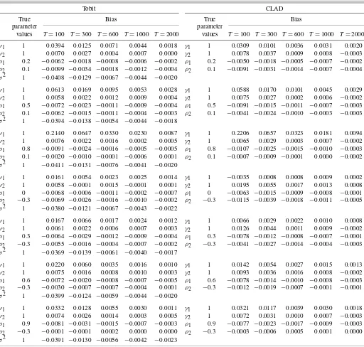
5. SIMULATIONS
Model: In this section, we evaluate the consistency of the Tobit and CLAD estimators of the dynamic censored regression model. We consider the data generating process
yt=max
0, γ1+γ2xt+ p
i=1
ρiyt−i+εt
,
where
xt=α1+α2xt−1+vt,
εt∼N(0, σε2),andvt∼N(0, σv2).For our simulations, we con-sider the cases p=1 andp=2. Many configurations for α1, α2, γ1,γ2, σv2,andσε2were considered. To conserve space, we
only report results forp=2, γ1=1, γ2=1, α1=α2=0.5, σε2=σv2=1. We conducted simulations for(ρ1, ρ2)∈{(0.2,
0.1),(0.5,0.1),(0.8,0.1),(0,−0.3),(0.3,−0.3),(0.6,−0.3), (0.9,−0.3)}. Note that, in contrast with Honoré and Hu (2004), in our simulations the values ofρiare not restricted to be non-negative. The number of replications used to compute the bias reported in the tables is 10,000.
Table1 reports the simulation results. For the dynamic To-bit model estimates of β =(ρ′, γ′, σε), with ρ′ =(ρ1, ρ2),
andγ′=(γ1, γ2)are obtained via maximum likelihood.
Pow-ell’s LAD estimates of the dynamic censored regression model whereβ=(ρ′, γ′),withρ′=(ρ1, ρ2), andγ′=(γ1, γ2)are
obtained using the BRCENS algorithm proposed by Fitzen-berger (1997a,1997b). As we mentioned in Section4, because
Table 1. Simulation results for censored regression model withp=2
Tobit CLAD
True Bias True Bias
parameter parameter
values T=100 T=300 T=600 T=1000 T=2000 values T=100 T=300 T=600 T=1000 T=2000
γ1 1 0.0394 0.0125 0.0071 0.0044 0.0018 γ1 1 0.0309 0.0101 0.0036 0.0031 0.0020 γ2 1 0.0070 0.0027 0.0004 0.0007 0.0000 γ2 1 0.0078 0.0037 0.0009 0.0008 −0.0003 ρ1 0.2 −0.0062 −0.0018 −0.0008 −0.0006 −0.0002 ρ1 0.2 −0.0050 −0.0018 −0.0005 −0.0007 −0.0002 ρ2 0.1 −0.0099 −0.0034 −0.0018 −0.0012 −0.0004 ρ2 0.1 −0.0091 −0.0031 −0.0014 −0.0007 −0.0004 σ2 1 −0.0408 −0.0129 −0.0067 −0.0044 −0.0020
γ1 1 0.0613 0.0169 0.0095 0.0053 0.0028 γ1 1 0.0588 0.0170 0.0101 0.0045 0.0029 γ2 1 0.0058 0.0022 0.0012 0.0009 0.0004 γ2 1 0.0075 0.0027 0.0002 0.0006 −0.0002 ρ1 0.5 −0.0072 −0.0023 −0.0011 −0.0009 −0.0004 ρ1 0.5 −0.0091 −0.0015 −0.0011 −0.0007 −0.0003 ρ2 0.1 −0.0062 −0.0015 −0.0011 −0.0004 −0.0003 ρ2 0.1 −0.0041 −0.0024 −0.0010 −0.0003 −0.0003 σ2 1 −0.0394 −0.0138 −0.0054 −0.0044 −0.0018
γ1 1 0.2140 0.0647 0.0330 0.0230 0.0087 γ1 1 0.2206 0.0657 0.0323 0.0181 0.0094 γ2 1 0.0076 0.0022 0.0016 0.0002 0.0005 γ2 1 0.0065 0.0029 0.0003 0.0007 −0.0002 ρ1 0.8 −0.0091 −0.0024 −0.0016 −0.0005 −0.0005 ρ1 0.8 −0.0107 −0.0025 −0.0015 −0.0010 −0.0003
ρ2 0.1 −0.0020 −0.0010 −0.0001 −0.0006 0.0001 ρ2 0.1 −0.0007 −0.0009 −0.0001 0.0000 −0.0002 σ2 1 −0.0411 −0.0131 −0.0076 −0.0041 −0.0020
γ1 1 0.0161 0.0054 0.0023 0.0025 0.0014 γ1 1 −0.0035 0.0008 0.0008 0.0009 0.0002 γ2 1 0.0058 −0.0001 0.0015 −0.0001 0.0001 γ2 1 0.0195 0.0055 0.0017 0.0013 0.0008 ρ1 0 −0.0068 −0.0006 −0.0011 −0.0002 −0.0007 ρ1 0 −0.0063 −0.0015 −0.0009 −0.0008 −0.0001 ρ2 −0.3 −0.0069 −0.0026 −0.0016 −0.0010 −0.0002 ρ2 −0.3 −0.0115 −0.0039 −0.0018 −0.0011 −0.0005 σ2 1 −0.0380 −0.0121 −0.0067 −0.0043 −0.0022
γ1 1 0.0167 0.0066 0.0017 0.0024 0.0012 γ1 1 0.0066 0.0029 0.0022 0.0010 0.0008 γ2 1 0.0061 0.0022 0.0006 0.0007 0.0003 γ2 1 0.0126 0.0044 0.0011 0.0009 −0.0002
ρ1 0.3 −0.0064 −0.0029 −0.0012 −0.0009 −0.0004 ρ1 0.3 −0.0078 −0.0012 −0.0008 −0.0007 −0.0001 ρ2 −0.3 −0.0055 −0.0016 −0.0004 −0.0007 −0.0002 ρ2 −0.3 −0.0041 −0.0027 −0.0014 −0.0004 −0.0003 σ2 1 −0.0369 −0.0139 −0.0061 −0.0040 −0.0017
γ1 1 0.0220 0.0060 0.0035 0.0016 0.0010 γ1 1 0.0142 0.0054 0.0027 0.0015 0.0013 γ2 1 0.0075 0.0016 0.0008 0.0010 0.0003 γ2 1 0.0093 0.0036 0.0016 0.0008 −0.0002 ρ1 0.6 −0.0072 −0.0020 −0.0008 −0.0007 −0.0005 ρ1 0.6 −0.0078 −0.0014 −0.0010 −0.0008 −0.0003 ρ2 −0.3 −0.0030 −0.0007 −0.0007 −0.0004 0.0001 ρ2 −0.3 −0.0012 −0.0019 −0.0007 −0.0001 −0.0001 σ2 1 −0.0399 −0.0124 −0.0059 −0.0044 −0.0020
γ1 1 0.0332 0.0128 0.0055 0.0030 0.0011 γ1 1 0.0321 0.0117 0.0039 0.0030 0.0018 γ2 1 0.0074 0.0026 0.0014 0.0003 0.0005 γ2 1 0.0072 0.0031 0.0010 0.0007 −0.0003 ρ1 0.9 −0.0081 −0.0031 −0.0015 −0.0007 −0.0003 ρ1 0.9 −0.0077 −0.0023 −0.0017 −0.0009 −0.0003 ρ2 −0.3 −0.0001 −0.0001 0.0002 0.0000 0.0000 ρ2 −0.3 −0.0003 −0.0006 0.0005 0.0001 0.0000 σ2 1 −0.0391 −0.0130 −0.0056 −0.0042 −0.0023
NOTE: yt=max(0, γ1+γ2∗xt+ρ1∗yt−1+ρ2∗yt−2+εt),xt=0.5+0.5xt−1+vt.
Powell’s LAD estimator does not provide a first-round estima-tor ofσε we redefineβ as to not includeσε.We report results
forT=100,300,600,1000,2000.
The simulations reveal that the maximum likelihood estima-tor for the dynamic Tobit model and Powell’s LAD estimaestima-tor of the dynamic censored regression model perform well for
T≥300 (see Table1). As expected, the bias decreases as the sample size increases.
6. EMPIRICAL APPLICATION
Without having considered formal issues of stationarity, Demiralp and Jordà (2002) estimated a dynamic Tobit model to analyze whether the February 4, 1994 Fed decision to publicly announce changes in the federal funds rate target affected the manner in which the Open Market Desk conducts operations. In what follows we reevaluate their findings.
6.1 Data and Summary of Previous Results
The data used by Demiralp and Jordà (2002) are daily and span the period between April 25, 1984 and August 14, 2000. They divide the sample in three subsamples: (i) the period pre-ceding the Fed decision to publicly announce changes in the federal fund rate target on February 4, 1994; (ii) the days be-tween February 4, 1994 and the decision to shift from con-temporaneous reserve accounting (CRA) to lagged reserves ac-counting (LRA) system in August 17, 1998; and (iii) the period following the shift to the CRA system.
Open market operations are classified in six groups. Oper-ations that add liquidity are overnight reversible repurchase agreements, term repurchase agreements, and permanent pur-chases (i.e., T-bill purpur-chases and coupon purpur-chases). Operations that drain liquidity are overnight sales, term matched-sale pur-chases, and permanent sales (i.e., T-bill sales and coupon sales). Because the computation of reserves is based on a 14-day main-tenance period that starts on Thursday and finishes on the “Set-tlement Wednesday” two weeks later, the maintenance-period average is the object of attention of the Open Market Desk. Thus, all operations are adjusted according to the number of days spanned by the transaction, and standardized by the ag-gregate level of reserves held by depository institutions in the maintenance period previous to the execution of the transaction. Demiralp and Jordà (2002) separate deviations of the fed-eral funds rate from the target into three components:NEEDt=
ft− [fm∗(t)−1+wtEm(t)−1(f
tenance period to which observation in daytbelongs,ft is the federal funds rate in dayt;fm∗(t)−1is the value of the target in the previous maintenance period;Em(t)−1(fm∗(t))is the expectation
of a target change in dayt, conditional on the information avail-able at the beginning of the maintenance period; andwt is the probability of a target change on datet.[Em(t)−1(fm∗(t))andwt are both calculated using the ACH model of Hamilton and Jordà (2002).] This decomposition reflects three different motives for open market purchases: (1) to add or drain liquidity in order to accommodate shocks to the demand for reserves; (2) to accom-modate expectations of future changes in the target; and (3) to adjust to a new target level. Thus,NEEDt represents a proxy
for the projected reserve need, and changes in the federal funds rate are separated into an expected component,EXPECTt, and a surprise component,SURPRISEt.
Because the Open Market Desk engaged in open market op-erations on 60% of the days in the sample (i.e., the data is cen-sored at zero during a large number of days), Demiralp and Jordà (2002) use a Tobit model to analyze the reaction func-tion of the Open Market Desk. To allow for a different response of sales and purchases—with varying degrees of permanence— to changes in the explanatory variables they estimate separate regressions for each of the six types of operation and each of the periods of interest. Very few term and permanent sales were carried out during the 1998–2000 and 1984–1994 periods re-spectively, thus no regressions are estimated for this type of operation in these subsamples. Demiralp and Jordà (2002) esti-mate the following model:
where yt denotes one of the open market operation of in-terest, that is, yt equals either overnight purchases (OBt), term purchases (TBt), permanent purchases (PBt), overnight sales (OSt), term sales (TSt), or permanent sales (PSt). zt denotes a vector containing the remaining five types of op-erations. For instance, if yt = OBt (overnight purchases), thenzt= [TBt,PBt,OSt,TSt,PSt].DAYtm denotes a vector of maintenance-day dummies, andεtis a stochastic disturbance.
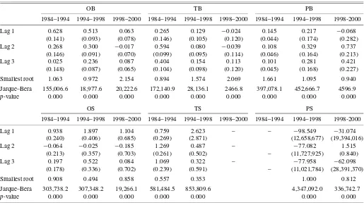
We start our empirical analysis by reestimating Demiralp and Jordà’s (2002) specifications under the assumption of normal-ity. That is, we follow their lead in assuming the dynamic To-bit model is correctly specified. We report the coefficient esti-mates for the lags of the dependent variable in Table2. (For the complete set of parameter estimates, see Tables A.1 and A.2 in the full version of this paper at http:// www.clas.wayne. edu/ herrera/ andhttp:// www.econ.ohio-state.edu/ dejong.) Be-cause we are interested in whether the roots of the polynomial ρmax(z)=1−3i=1max(0, ρi)ziare outside the unit circle we report the smallest of the moduli of the roots of this lag polyno-mial.
Note that 10 out of the 16 regressions estimated by Demi-ralp and Jordà (2002) appear to have at least one root that falls on or inside the unit circle. One may wonder whether this re-sult stems from nonstationarity issues or from misspecification in the error distribution. To investigate this issue, we test for normality of the Tobit residuals and report the Jarque–Bera sta-tistics in Table 1; these results lead us to reject the null that the underlying disturbances are normally distributed. Thus, we proceed in the following section to estimate the Open Market
234 Journal of Business & Economic Statistics, April 2011
Table 2. Demiralp and Jordà (2002) Tobit regression for Open Market operations coefficient estimates for lags of the dependent variable
OB TB PB
1984–1994 1994–1998 1998–2000 1984–1994 1994–1998 1998–2000 1984–1994 1994–1998 1998-2000
Lag 1 0.628 0.513 0.063 0.265 0.129 −0.024 0.145 0.217 −0.068
(0.141) (0.093) (0.078) (0.146) (0.105) (0.120) (0.044) (0.174) (0.282)
Lag 2 0.268 0.300 −0.017 0.594 0.080 −0.039 0.108 0.329 0.737
(0.146) (0.091) (0.070) (0.099) (0.095) (0.114) (0.046) (0.164) (0.213)
Lag 3 0.025 0.236 0.087 0.404 0.154 0.113 0.101 0.281 0.421
(0.148) (0.087) (0.065) (0.104) (0.098) (0.120) (0.045) (0.168) (0.227)
Smallest root 1.063 0.972 2.154 0.894 1.574 2.069 1.661 1.095 0.940
Jarque–Bera 155,006.6 18,977.6 20,222.6 172,140.9 28,136.1 2466.8 397,078.1 452,666.7 4596.9
p-value 0.000 0.000 0.000 0.000 0.000 0.000 0.000 0.000 0.000
OS TS PS
1984–1994 1994–1998 1998–2000 1984–1994 1994–1998 1998–2000 1984–1994 1994–1998 1998-2000
Lag 1 0.938 1.897 1.104 0.759 2.623 – – −98.549 −31.074
(0.240) (0.406) (0.685) (0.269) (2.871) (12,658,677) (19,394,016)
Lag 2 −0.064 −0.025 −0.185 1.269 0.487 – −77.082 1.515
(0.213) (0.357) (0.703) (0.261) (0.502) – (11,727,925) (0.840)
Lag 3 0.197 0.522 0.084 1.069 0.322 – −77.958 −62.098
(0.178) (0.336) (0.702) (0.239) (0.591) – (11,021,784) (28,391,370)
Smallest root 0.908 0.494 0.858 0.557 0.353 1.000 0.812
Jarque–Bera 303,738.2 307,348.2 19,266.1 581,484.5 853,809.6 4,347,092.0 336,742.7
p-value 0.000 0.000 0.000 0.000 0.000 0.000 0.000
NOTE: Standard errors reported in parenthesis. Smallest root denotes the smallest root ofρmax(z)polynomial; for complex roots the modulus is reported.
Desk’s reaction function using Powell’s LAD estimator, which is robust to unknown error distributions. If the problem is one of nonstationarity, one would then expect the roots of theρmax(·)
polynomial to be on or inside the unit circle.
6.2 Model and Estimation Procedure
From here on we will restrict our attention to the Open Mar-ket Desk’s reaction function for temporary open marMar-ket pur-chases over the whole 1984–2000 sample. We focus on tem-porary purchases because overnight and term RPs are the most common operations; thus, they are informative regarding the Open Market Desk’s reaction function. The Open Market Desk engaged in temporary purchases on 37% of the days between April 25, 1984 and August 14, 2000. In contrast, permanent purchases, temporary sales, and permanent sales were carried out, respectively, on 24%, 7%, and 2% of the days in the sam-ple.
In contrast with Demiralp and Jordà (2002) we reclassify open market operations in four groups: (a) temporary pur-chases, which comprise overnight reversible repurchase agree-ments (RP) and term RP,OTBt=OBt+TBt; (b) permanent pur-chases, which include T-bill purchases and coupon purpur-chases,
PBt; (c) temporary sales, which include overnight and term matched sale-purchases,OTSt=OSt+TSt; and (d) permanent sales, which comprise T-bill sales and coupon sales, PSt. In brief, we group overnight and term operations and restrict our analysis to the change in the maintenance-period-average level of reserves brought about by temporary purchases of the Open Market Desk,OTBt.
We employ the following dynamic censored regression model to describe temporary purchases by the Open Market Desk:
OTBt=max
0, γ+
4
m=1
γmαDtm+
3
j=1
ρjOTBt−j
+
3
j=1
γjTSOTSt−j+
3
j=1
γjPBPBt−j+
3
j=1
γjPSPSt−j
+
10
m=1
γmNNEEDt−m×DAYtm
+
10
m=1
γmEEXPECTt−m×DAYtm
+
3
j=0
γjSSURPRISEt−j+εt
, (15)
whereOTBt denotes temporary purchases,OTSt denotes tem-porary sales, PBt denotes permanent purchases, PSt denotes permanent sales,DAYtm denotes a vector of maintenance-day dummies, Dtm is such that Dt1 =DAYt1 (First Thursday), Dt2=DAYt2(First Friday),Dt3=DAYt7(Second Friday),and Dt4=DAYt,10 (Settlement Wednesday), andεt is a stochastic disturbance.
This model is a restricted version of (14) in that it does not in-clude dummies for all days in the maintenance period. Instead, to control for differences in the reserve levels that the Federal Reserve might want to leave in the system at the end of the day,
we include only dummies for certain days of the maintenance period where the target level of reserves is expected to be dif-ferent from the average (see Demiralp and Farley2005).
Regarding the estimation procedure, Tobit estimates b are obtained in the usual manner via maximum likelihood esti-mation, whereas the CLAD estimatesb are obtained by us-ing the BRCENS algorithm proposed by Fitzenberger (1997a, 1997b). Extensive Monte Carlo simulations by Fitzenberger (1997a) suggest that this algorithm, which is an adaptation of the Barrodale–Roberts algorithm for the censored quantile re-gression, performs better than the iterative linear programming algorithm (ILPA) of Buchinsky (1994) and the modified ILPA algorithm (MILPA) of Fitzenberger (1994), in terms of the per-centage of times it detects the global minimum of a censored quantile regression. In fact, for our application, a grid search over 1000 points in the neighborhood of the estimatesb indi-cates both the ILPA and MILPA algorithms converge to a local minimum. In contrast, the BRCENS algorithm is stable and ap-pears to converge to a global minimum.
Because the CLAD does not provide a first-round estimate for the variance, N−1N−1, we compute it in the following manner.is calculated as the long-run variance ofψ (wt,b)=
I(b′wt>0)[12 −I(yt<b′wt)]wt,following the suggestions of Andrews (1991) to select the bandwidth for the Bartlett ker-nel. To computeN, we estimatef(0|wt)using a higher-order Gaussian kernel with the order and bandwidth selected accord-ing to Hansen (2003,2004).
6.3 Estimation Results
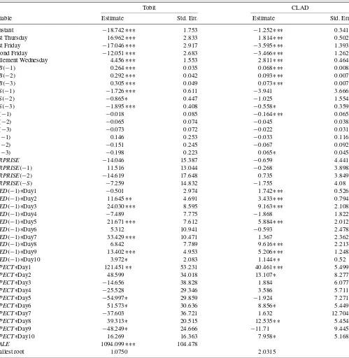
Maximum likelihood estimates of the dynamic Tobit model and corresponding quasi-maximum likelihood standard errors are presented in the first two columns of Table3. Before we comment on the estimation results, it is important to inspect whether the roots of the lag polynomial ρmax(z) lie outside
the unit circle. The three roots of ρmax(z)=1−0.2639z−
0.2916z2−0.3054z3lie all outside the unit circle, and the small-est modulus of these roots equals 1.075. Because this root is near the unit circle and because we do not have the tools to test if it is statistically greater than one, we should proceed with caution.
Of interest is the presence of statistically significant coeffi-cients on the lags of the dependent variable,TBt−j. This
persis-tence suggests that in order to attain the desired target, the Open Market Desk had to exercise pressure on the fed funds market in a gradual manner, on consecutive days. The negative and statis-tically significant coefficients on lagged temporary sales,TSt−j, imply that temporary sales constituted substitutes for temporary purchases. In other words, in the face of a reserve shortage the Open Market Desk could react by conducting temporary pur-chases and/or delaying temporary sales. The positive and statis-tically significant coefficients on theNEEDt−1×DAYtm vari-ables is consistent with an accommodating behavior of the Fed to deviations of the federal funds rate from its target. The Tobit estimates suggest that expectations of target changes were ac-commodated in the first days of the maintenance period, and did not significantly affect temporary purchases on most of the re-maining days. As for the effect of surprise changes in the target,
the estimated coefficients are statistically insignificant. Accord-ing to Demiralp and Jordà (2002), statistically insignificant co-efficients onSURPRISEt−jcan be interpreted as evidence of the announcement effect. This suggests that the Fed did not require temporary purchases to signal the change in the target, once it had been announced (or inferred by the markets; see Demiralp and Jordà2004).
However, it is well known that the Tobit estimates are in-consistent if the underlying disturbances are heteroskedastic or nonnormal (Greene 2000). Thus, to assess whether the Tobit specification of the reaction function is appropriate, we conduct tests for homoscedasticity and normality. A Lagrange multiplier test of heteroscedasticity obtained by assuming Var(εt|wt)= σ2exp(δ′zt), wherezt is a vector that contains all elements in
wt but the constant, rejects the nullH0:δ=0 at the 1% level.
In addition, the Jarque–Bera statistic leads us to reject the null that the residuals are normally distributed at a 1% level.
The finding of a root that is close to the unit circle in con-junction with the rejection of the normality and homoscedas-ticity assumptions suggest that the Tobit estimates could be bi-ased. Hence, our finding of a root near the unit circle may stem either from misspecification of the error term or from nonsta-tionarity of the dynamic Tobit model. To further investigate this issue, we consider the CLAD estimator, which is robust to heteroscedasticity and nonnormality and is consistent in the presence of weakly dependent errors (see Section4). Finding a root close to unity for the CLAD estimates would be indicative of nonstationarity in the dynamic censored regression model driving the test results. In contrast, finding roots that are out-side the unit circle would point towards misspecification of the error distribution being the cause of the bias in the Tobit esti-mates.
CLAD estimates and corresponding standard errors are re-ported in the third and fourth column of Table3, respectively. Notice that, in this case, the smallest root of the lag polyno-mialρmax(z)=1−0.068z−0.093z2−0.073z3appears to be
clearly outside the unit circle. Here the smallest modulus of the roots equals 1.928. Given that the roots are far from the unit circle, standard inference techniques seem to be asymptotically justified. Furthermore, this suggest that our finding of roots that are near the unit circle for the Tobit model is a consequence of misspecification in the error term as normal and homoscedas-tic.
Comparing the CLAD and the Tobit estimates reveals some differences regarding the Open Market Desk’s reaction func-tion. First, the CLAD estimates imply a considerably smaller degree of persistence in temporary purchases. The magnitude of the ρj, j=1,2,3, parameter estimates is at most 1/3 of the Tobit estimates. Consequently, the roots of the lag polyno-mialρmax(z)implied by the CLAD estimates are larger, giving
us confidence regarding stationarity of the censored regression model.
Second, although both estimates imply a similar reaction of the Fed to reserve needs, there are some differences in the mag-nitude and statistical significance of the parameters. In partic-ular, the CLAD estimates suggest a pattern in which the Fed is increasingly less reluctant to intervene during the first three days of the maintenance period; then, no significant response is apparent for the following four days (with the exception of
236 Journal of Business & Economic Statistics, April 2011
Table 3. Tobit and CLAD estimates of Open Market temporary purchases
Tobit CLAD
Variable Estimate Std. Err. Estimate Std. Err.
Constant −18.742∗∗∗ 1.753 −1.252∗∗∗ 0.341
First Thursday 16.962∗∗∗ 2.833 1.814∗∗∗ 0.502
First Friday −17.046∗∗∗ 2.917 −3.595∗∗∗ 1.393
Second Friday −12.051∗∗∗ 2.683 −3.466∗∗∗ 1.262
Settlement Wednesday 4.456∗∗∗ 1.553 2.811∗∗∗ 0.464
OTB(−1) 0.264∗∗∗ 0.035 0.068∗∗∗ 0.008
OTB(−2) 0.292∗∗∗ 0.042 0.093∗∗∗ 0.007
OTB(−3) 0.305∗∗∗ 0.049 0.073∗∗∗ 0.007
OTS(−1) −1.726∗∗∗ 0.611 −3.941 3.666
OTS(−2) −0.865∗ 0.447 −1.025 1.554
OTS(−3) −1.895∗∗∗ 0.408 −0.558∗ 0.359
PB(−1) −0.018 0.085 −0.164∗∗∗ 0.065
PB(−2) −0.065 0.074 −0.045 0.038
PB(−3) −0.073 0.072 −0.022 0.031
PS(−1) 0.146 0.253 −0.033 0.116
PS(−2) −0.151 0.245 −0.067 0.092
PS(−3) −0.198 0.223 0.065∗ 0.045
SURPRISE −14.046 15.387 −0.659 4.441
SURPRISE(−1) 11.516 13.044 −0.268 3.898
SURPRISE(−2) −14.619 17.648 0.735 3.849
SURPRISE(−S) −7.259 14.832 −1.755 4.08
NEED(−1)∗Day1 −0.501 2.974 1.742∗∗∗ 0.526
NEED(−1)∗Day2 11.645∗∗ 4.691 3.433∗∗∗ 0.794
NEED(−1)∗Day3 24.030∗∗∗ 8.595 9.163∗∗∗ 2.108
NEED(−1)∗Day4 −7.489 7.775 −1.868 1.822
NEED(−1)∗Day5 21.671∗∗∗ 7.612 5.884∗∗∗ 2.012
NEED(−1)∗Day6 5.312 10.941 −0.593 2.478
NEED(−1)∗Day7 33.429∗∗∗ 10.471 1.367 2.362
NEED(−1)∗Day8 6.842 7.789 9.616∗∗∗ 2.213
NEED(−1)∗Day9 13.402∗∗∗ 4.953 5.206∗∗∗ 1.248
NEED(−1)∗Day10 3.972∗ 2.083 1.144∗∗ 0.52
EXPECT∗Day1 121.451∗∗ 53.231 40.461∗∗∗ 5.499
EXPECT∗Day2 48.599 34.018 13.107∗ 8.277
EXPECT∗Day3 −14.656 38.828 1.884 6.077
EXPECT∗Day4 −25.528 29.346 3.586 5.711
EXPECT∗Day5 −54.997∗ 29.859 −1.924 7.271
EXPECT∗Day6 51.573∗ 30.636 8.856∗ 5.449
EXPECT∗Day7 −37.603 36.721 1.632 12.704
EXPECT∗Day8 39.313∗ 20.515 12.535∗∗ 5.454
EXPECT∗Day9 −48.249∗ 24.666 −11.71 9.445
EXPECT∗Day10 16.269 16.363 7.958∗ 5.168
SCALE 1094.099∗∗∗ 104.478
Smallest root 1.0750 2.0315
NOTE: ∗ ∗ ∗,∗∗, and∗denote significance at the 1,5, and 10% level, respectively. Smallest root denotes the smallest root of theρmax(z)polynomial; for complex roots the modulus is reported.
Day 5); finally, the response to reserve needs becomes positive and significant for the last three days of the period. Further-more, on Mondays (Day 3 and Day 8), the Open Market Desk appears to be more willing to accommodate shocks in the de-mand for reserves in order to maintain the federal funds rate aligned with the target.
The expectation of a change in the target seldom triggers tem-porary open market purchases. The coefficient onEXPECT is only statistically significant on the first and eighth day of the maintenance period. This suggests the Fed is only seldom will-ing to accommodate (or profit) from anticipated changes in the
target. Although both estimation methods reveal a larger effect on the first day, the CLAD estimate (40.5) suggest an impact that is about 67% smaller than the Tobit estimate (121.5).
Most of the coefficients on the contemporaneous and lagged
SURPRISEare negative, which is consistent with the liquidity effect. That is, in order to steer the federal funds rate towards a new lower target level the Open Market Desk would add liq-uidity by using temporary purchases. Yet, the fact that none of the coefficients are statistically significant suggests that once the target was announced (or inferred by the financial markets) little additional pressure was needed to enforce the new target.
7. CONCLUSIONS
This paper shows stationarity properties of the dynamic cen-sored regression model in a time series framework. It then pro-vides a formal justification for maximum likelihood estimation of the dynamic Tobit model and for Powell’s LAD estimation of the dynamic censored regression model, showing consistency and asymptotic normality of both estimators. Two important features of the treatment of the censored regression model in this paper is that no assumption is made on the lag polynomial other than thatρmax(z)=1−ip=1max(0, ρi)zi has its roots
outside the unit circle and that the error term, εt, is itself al-lowed to be potentially correlated. Hence, in terms of the con-ditions onρmax(z)and the dependence allowed forεt, this paper analyzes the dynamic censored regression model on a level of generality that is comparable to the level of generality under which results for the linear model AR(p) model can be derived. The censored regression model is then applied to study the Open Market Desk’s reaction function. Robust estimates for temporary purchases using Powell’s CLAD suggest that max-imum likelihood estimates of the dynamic Tobit model may lead to overestimating the persistence of temporary purchases, as well as the effect of demand for reserves and expectations of future changes in the federal funds target on temporary pur-chases. Moreover, a comparison of the Tobit and CLAD esti-mates suggests that temporary purchases are stationary, but that the error normality assumed in the Tobit specification does not hold.
SUPPLEMENTAL MATERIALS
Appendix: Mathematical appendix containing all proofs for this paper. (appendix.pdf)
Full version: Full and detailed version of this paper. (full.pdf)
ACKNOWLEDGMENTS
We thank Selva Demiralp and Oscar Jordà for making their data available, and Bruce Hansen for the use of his code for kernel density estimation.
[Received August 2007. Revised May 2009.]
REFERENCES
Amemiya, T. (1973), “Regression Analysis When the Dependent Variable Is Truncated Normal,”Econometrica, 41, 997–1016. [228]
Andrews, D. W. K. (1991), “Heteroskedasticity and Autocorrelation Consistent Covariance Matrix Estimation,”Econometrica, 59, 817–858. [235] Arellano, M., and Honoré, B. (1998), “Panel Data Models: Some Recent
De-velopments,” inHandbook of Econometrics, Vol. 5, eds. J. J. Heckman and E. Leamer, Amsterdam: North-Holland, Chapter 53. [228,229]
Bougerol, P., and Picard, N. (1992), “Strict Stationarity of Generalized Autore-gressive Processes,”The Annals of Probability, 20, 1714–1730. [230] Buchinsky, M. (1994), “Changes in the U.S. Wage Structure 1963–1987:
Ap-plication of Quantile Regression,”Econometrica, 62, 405–458. [235]
Chavas, J.-P., and Kim, K. (2006), “An Econometric Analysis of the Effects of Market Liberalization on Price Dynamics and Price Volatility,”Empirical Economics, 31, 65–82. [229]
Davidson, J. (1994),Stochastic Limit Theory, Oxford: Oxford University Press. [230]
de Jong, R. M., and Woutersen, T. (2010), “Dynamic Time Series Binary Choice,”Econometric Theory, to appear. [229]
Demiralp, S., and Farley, D. (2005), “Declining Required Reserves, Funds Rate Volatility, and Open Market Operations,”Journal of Banking and Finance, 29, 1131–1152. [235]
Demiralp, S., and Jordà, O. (2002), “The Announcement Effect: Evidence From 69 Open Market Desk Data,”Economic Policy Review, 8, 29–48. [229,233-235]
(2004), “The Response of Term Rates to Fed Announcements,” Jour-nal of Money, Credit, and Banking, 36, 387–406. [235]
Fitzenberger, B. (1994), “A Note on Estimating Censored Quantile Regres-sions,” Discussion Paper 14, University of Konstanz. [235]
(1997a), “Computational Aspects of Censored Quantile Regression,” in Proceedings of the 3rd International Conference on Statistical Data Analysis Based on the L1-Norm and Related Methods, ed. Y. Dodge, Hay-ward, CA: IMS, pp. 171–186. [232,235]
(1997b), “A Guide to Censored Quantile Regressions,” inHandbook of Statistics, Vol. 14, Amsterdam: North-Holland, pp. 405–437. [232,235] Frenkel, M., Pierdzioch, C., and Stadtmann, G. (2003), “Modeling Coordinated
Foreign Exchange Market Interventions: The Case of the Japanese and U.S. Interventions in the 1990s,”Review of World Economics, 139, 709–729. [229]
Gallant, A. R., and White, H. (1988),A Unified Theory of Estimation and In-ference for Nonlinear Dynamic Models, New York: Blackwell. [230] Greene, W. (2000),Econometric Analysis(5th ed.), Upper Saddle River, NJ:
Prentice-Hall. [235]
Hamilton, J. D., and Jordà, O. (2002), “A Model for the Federal Funds Rate Target,”Journal of Political Economy, 110, 1135–1167. [233]
Hansen, B. E. (1996), “Stochastic Equicontinuity for Unbounded Dependent Heterogeneous Arrays,”Econometric Theory, 12, 347–359. [231]
(2003), “Exact Mean Integrated Square Error of Higher-Order Kernel Estimators,” working paper, University of Wisconsin. [235]
(2004), “Bandwidth Selection for Nonparametric Kernel Estimation,” working paper, University of Wisconsin. [235]
Honoré, B., and Hu, L. (2004), “Estimation of Cross Sectional and Panel Data Censored Regression Models With Endogeneity,”Journal of Econometrics, 122, 293–316. [228,229,232]
Kim, S., and Sheen, J. (2002), “The Determinants of Foreign Exchange Inter-vention by Central Banks: Evidence From Australia,”Journal of Interna-tional Money and Finance, 21, 619–649. [229]
Kodres, L. E. (1988), “Test of Unbiasedness in the Foreign Exchange Futures Markets: The Effects of Price Limits,”Review of Futures Markets, 7, 139– 166. [229]
(1993), “Test of Unbiasedness in the Foreign Exchange Futures Mar-kets: An Examination of Price Limits and Conditional Heteroscedasticity,”
Journal of Business, 66, 463–490. [229]
Lee, L.-F. (1999), “Estimation of Dynamic and ARCH Tobit Models,”Journal of Econometrics, 92, 355–390. [229]
Meyn, S. P., and Tweedie, R. L. (1994),Markov Chains and Stochastic Stability
(2nd ed.), Berlin: Springer-Verlag. [228]
Pötscher, B. M., and Prucha, I. R. (1997),Dynamic Nonlinear Econometric Models, Berlin: Springer-Verlag. [230]
Powell, J. L. (1984), “Least Absolute Deviations Estimation for the Censored Regression Model,”Journal of Econometrics, 25, 303–325. [229] Wei, S. X. (1999), “A Bayesian Approach to Dynamic Tobit Models,”
Econo-metric Reviews, 18, 417–439. [229]
(2002), “A Censored-Garch Model of Asset Returns With Price Lim-its,”Journal of Empirical Finance, 9, 197–223. [229]
Zangari, P. J., and Tsurumi, H. (1996), “A Bayesian Analysis of Censored Au-tocorrelated Data on Exports of Japanese Passenger Cars to the United States,” inBayesian Computational Methods and Applications. Advances in Econometrics, Vol. 11 (Part A), Bingley, U.K.: Emerald, pp. 111–143. [229]