Full Terms & Conditions of access and use can be found at
http://www.tandfonline.com/action/journalInformation?journalCode=ubes20
Download by: [Universitas Maritim Raja Ali Haji] Date: 11 January 2016, At: 22:58
Journal of Business & Economic Statistics
ISSN: 0735-0015 (Print) 1537-2707 (Online) Journal homepage: http://www.tandfonline.com/loi/ubes20
An Econometric Analysis of Some Models for
Constructed Binary Time Series
Don Harding & Adrian Pagan
To cite this article: Don Harding & Adrian Pagan (2011) An Econometric Analysis of Some
Models for Constructed Binary Time Series, Journal of Business & Economic Statistics, 29:1, 86-95, DOI: 10.1198/jbes.2009.08005
To link to this article: http://dx.doi.org/10.1198/jbes.2009.08005
Published online: 01 Jan 2012.
Submit your article to this journal
Article views: 269
An Econometric Analysis of Some Models for
Constructed Binary Time Series
Don H
ARDINGLatrobe University, Bundoora, Australia 3056 (d.harding@latrobe.edu.au)
Adrian P
AGANUniversity of New South Wales, Sydney, Australia, 2052 and Queensland University of Technology, Brisbane, Australia, 4000 (A.Pagan@unsw.edu.au)
Macroeconometric and financial researchers often use binary data constructed in a way that creates serial dependence. We show that this dependence can be allowed for if the binary states are treated as Markov processes. In addition, the methods of construction ensure that certain sequences are never observed in the constructed data. Together these features make it difficult to utilize static and dynamic Probit models. We develop modeling methods that respect the Markov-process nature of constructed binary data and ex-plicitly deals with censoring constraints. An application is provided that investigates the relation between the business cycle and the yield spread.
KEY WORDS: Binary variable; Business cycle; Markov process; Probit model; Yield curve.
1. INTRODUCTION
Macroeconometric and financial econometric research often feature discrete random variables that were constructed from some underlying continuous random variable yt. Often these
discrete variables have a binary form, with the two values rep-resenting whether an event has occurred or not. An example might be the sign of the change in an interest rate. Such a con-structed variable has anordinalnature. There are other cases where the discrete random variable is augmented in such a way as to make itcardinal, e.g., by identifying the actual values of the signed changes inytas the outcomes of the discrete random
variable. An influential example is Eichengreen, Watson, and Watson(1985) who implemented such a strategy for the mod-eling of Bank Rate—the rate of interest charged by the Bank of England to discount houses and other dealers in Treasury bills—as this rate only varied by a small number of discrete movements. If the constructed variables have a cardinal nature then the methods to analyze them are clearly different from the ordinal case, as extra information is available. This article is concerned with the analysis of ordinal binary variables. The na-ture of such constructed random variables has not been stud-ied much, the notable exceptions being Kedem (1980), Watson (1994), Startz (2008), and Harding and Pagan (2006).
The binary variable we will work with can be thought of as representing the state of some characteristic of the economic and financial system, such as activity or equity market perfor-mance. We designate it asSt. As an example data on economic
activity can be used to construct a binary variable St, taking
the value of unity if activity is in an expansion phase and zero when activity is in the contraction phase. Although there are many other examples, including bull and bear markets for stock prices, we focus mainly on the case of economic activity, i.e., business cycles.
The dataStare mostly constructed by some individuals and
agencies that are external to the researcher. A question that then arises is whether the methods of construction have an impact upon the data generating process (DGP) of the St, and if so,
do these features create any special problems for economet-ric analysis? To make this question more concrete, consider the business cycle data available from the National Bureau of Eco-nomic Research (NBER). Using the quarterlyStthey present on
their web page for 1959/1 to 1995/2 (the same period as in the application we look at in Section5), an ordinary least squares (OLS) regression that is run in Equation (1) ofSton a constant, St−1,St−2, andSt−1St−2[Newey–West (1987) HACt-ratios in
brackets for window width four],
St= 0.4
(3.8)+0.(5.6)6St−1−0(−.4S3.8)t−2+0.35(3.1)St−1St−2+ut. (1) Equation (1) has three striking features. First, the estimated constant term and the coefficient ofSt−1 sum exactly to one.
Second, the estimated constant and the coefficient onSt−2sum
exactly to zero. In both cases these results hold exactly inde-pendently of the number of decimal places used to represent the coefficients. Third, the process forSt is, at least, a
second-order process. The question is where these features come from. In this article we show that the method of construction is an im-portant determinant of them and that models should be chosen that recognize that these features will be present.
In Section2of the article, we explore the interaction between the method of construction of theStand the nature of theytthey
are drawn from. We do so by looking at some simple rules for constructing theSt,which capture the main ways that such
vari-ables are constructed. We then interact these rules with a DGP for theyt chosen so that it mimics the data on the underlying
variables from which theStderive. The simple examples of this
section are meant to aid an understanding of the origin of the features above and to guide researchers when selecting appro-priate models for theSt.
© 2011American Statistical Association Journal of Business & Economic Statistics
January 2011, Vol. 29, No. 1 DOI:10.1198/jbes.2009.08005
86
Often we wish to relate these binary random variables to some regressorsxt. In such circumstances, the literature on
con-ditional models for categorical data is mostly employed. Pro-bit and Logit models are well known examples of this class. These relateSt to a single indexx′tθ, through Pr(St=1|xt)= F(x′tθ)=F(zt),whereF(·)is a cumulative distribution
func-tion with the properties thatF(z)is monotonic increasing inz, limz→−∞F(z)=0 and limz→∞F(z)=1.The Probit model is
the special case whereF(·)=(·),the cdf of the standard nor-mal. Mostly these are static models, as in Estrella and Mishkin (1998), but some dynamic versions were proposed to handle a time series of categorical data, e.g., Kauppi and Saikkonen (2008) and de Jong and Woutersen (2010). In these models, termed a single index dynamic categorical (SIDC) model here, one has Pr(St=1|xt,St−1, . . . ,St−p)=F(x′tθ,St−1, . . . ,St−p).
It is natural then to seek to utilize those models to describe the DGP of theSt.Using a popular rule for determining business
cycle dates, we show that the DGP of the binary states cannot be represented by the SIDC that has mostly been used. This raises doubts about whether the NBER business-cycle states can be represented in this way.
The issue just raised leads in Section3to a presentation of multiple index generalizations of the SIDC model, which can match the features of NBER binary data. These are termed GDC models. In Section4 we adapt a nonparametric estima-tion method to estimate the GDC model. Secestima-tion5then applies this method to the same sample of NBER data as used by Es-trella and Mishkin (1998) when fitting a single index static Pro-bit model. We find that the econometric issues originating from the method of construction of theSt that are identified
previ-ously are empirically significant.
2. THE IMPACT OF METHOD OF CONSTRUCTION ON THE DGP OF THE BINARY VARIABLES
Even though some information might be lost in the process, binary variables are constructed from a primary set of data for at least two purposes. One is to focus attention on particular characteristics. Thus, squaring the data loses information on the sign, but emphasizes volatility. In the same way, binary random variables locating expansions and recessions focus attention on the frequency and length of these extreme events. The second is to reduce the dimension of the DGP so as to more easily dis-cern important patterns in the data or to isolate characteristics that a model seeking to interpret the data will need to incorpo-rate. Thus, decomposing data such asytinto its permanent and
transitory components is a key step in economic model design. In the same way, an interaction of the binary data with theytcan
point to important characteristics such as the rapidity of recov-ery from an expansion that economic models need to account for.
Often the user of theStis not the producer. Consequently, the
researcher often just has a set of binary dataSt available and
(sometimes) knowledge of theyt they were constructed from.
To understand the nature of theStwe, therefore, need to have
some idea of the transformations that link these two series. Al-though we may not know precisely how this is done, in most instances enough information is provided along with the data
on theStto enable a good approximation to it. It is worth
think-ing of the conversion process from yt toSt as involving three
stages, and to see how the nature (DGP) ofSt changes at each
stage. We do this in the subsequent subsections.
2.1 Stage 1: Effects of State Change Rules
In the first stage we seek to determine what state the sys-tem is in at various points in the sample path. In the business cycle context, where we are seeking states of expansion and contraction, it is often the case that these are identified by lo-cating theturning pointsin the seriesyt.Often these first stage
turning points are produced by a set ofrulesformalized in al-gorithms such as that due to Bry and Boschan (BB) (1971) and a simplified quarterly version of it (BBQ) described in Harding and Pagan (2002). In other cases, the rules are found by using the output from fitting statistical models such as latent Markov processes to the yt series—Hamilton (1989). In all instances
these rules transformytintoSt.
Because turning point rules are widely used in the analysis of business cycles (and are the basis of the NBER data that we uti-lize later for empirical work) we focus on them in what follows. Turning points are found by locating the local maxima and min-ima in the seriesyt.A variety of rules appear in the literature
to produce the turning points. It is useful to study three of these in order to understand how each rule influences the nature of the univariate DGP for St and to understand the interrelations
betweenSt and any regressorsxt that are thought to influence
the state. The impact of any given rule will also depend upon the DGP ofyt.Consequently, we study how the mapping
be-tweenyt andSt changes as we modify either the rules or the
DGP ofyt.
2.1.1 Calculus Rule. The simplest method of locating turning points is what might be termed thecalculus rule. This says that a peak in a series on activity yt occurs at timet if yt>0 andyt+1<0.The reason for the name is the result
in calculus that identifies a maximum with a change in sign of the first derivative from being positive to negative. A trough (or local minimum) can be found using the outcomesyt<0
and yt+1>0. The states St are simply defined in this case
as St =1(yt >0), so that St depends only on
contempo-raneous information. Note that we can formulate this rule as St=1(yt>0|St−1= {0,1})in which case it describes how
the state changes, and it might be called a termination rule. This rule has been popular for defining a business cycle when ytis yearly data, see Cashin and McDermott (2002) and Neftci
(1984).
Univariate DGP of St. Suppose that yt is a Gaussian
covariance stationary process and the calculus rule is employed. In this instance, Kedem (1980, p. 34) set out the relation be-tween the autocorrelations of theyt andS(t)processes.
Let-tingρy(k)=corr(yt, yt−k),andρS(k)=corr(St,St−k),he
that the order of theStprocess changes with the degree of serial
correlation in theyt series. Since turning points are invariant
to monotonic transforms of the data, we can think ofytas being
88 Journal of Business & Economic Statistics, January 2011
the log of a variable such as activity. Hence, the degree of ser-ial correlation in the growth rates of activity will influence the cycle turning points found with the calculus rule.
Relation of St andxt. If the underlying process foryt
is
yt=x′tθ+εt, (3)
wherext is assumed to be strictly exogenous (and so can be
conditioned upon) andεt isnid(0,1).ThenSt=1(x′tθ+εt>
0) and a static Probit model will clearly capture the rela-tion between St and the single index zt=x′tθ since Pr(St=
1|zt,St−1)=(zt).
2.1.2 Two Quarters Rule. The rule that two quarters of negative growth terminates a recession is often cited in the me-dia. Extended so that the start of an expansion is identified with two quarters of positive growth produces the “two quar-ters rule”:
St=1 if(yt+1>0, yt+2>0|St−1=0),
St=0 if 1(yt+1<0, yt+2<0|St−1=1), (4)
St=St−1 otherwise.
Lunde and Timmermann (2004) used a variant of this nonpara-metric rule for finding bull and bear periods in stock prices while hot and cold markets for initial public offerings (IPO’s) were identified by Ibbotson and Jaffee (1975), with a hot mar-ket being signalled by whether excess returns and their changes for two periods exceed the median values.Eichengreen, Rose, and Wyplosz(1995) andClaessens, Kose, and Terrones(2008) employed rules of this type to establish the location of crises in time.
Univariate DGP of St. To illustrate the features of this
rule consider the case whereytis a Gaussian random walk with
drift
yt=μ+σet, (5)
whereetisnid(0,1)and Pr(yt<0)=(−σμ)≡ψ.Then, we
show in theAppendix Athat the first order representation ofSt
has the following parameterization
This example shows that even whereyt is a Gaussian random
walk the use of a two quarters rule rather than the calculus rule induces serial correlation into theStprocess so that it is at least
a first-order process.
Relation of St and xt. It is also instructive to examine
the case whereyt has the DGP in Equation (3). The
Appen-dix Aderives Pr(St=1|St−1=1,xt,xt−1, . . .), and it is found
to depend nonlinearly upon the complete history{xt−j}∞j=0, with
the nonlinear mapping failing to be that provided by the cdf of an N(0,1)variable. Hence, a static Probit model will be inap-propriate. A dynamic one, in which lags ofStare added to the
single index, will certainly imply dependence of the probability on past values ofxt,but the nonlinear mapping betweenStand
{xt−j}∞j=0 will be incorrect. For this reason, we need to allow
for a general functional relation connectingStandxt, and we,
therefore, set out methods for doing this in the next section.
2.1.3 Bry–Boschan and BBQ Rules. Neither the calculus rule nor the “two quarters” rule accurately describes the rule used by the NBER to locate local peaks and troughs inyt. To
match the features of that data requires a rule that formalizes the visual intuition that a local peak inyt occurs at timet if yt>ysforsin a windowt−k<s<t+k—a trough is defined
in a similar way. By makingklarge enough we also capture the idea that the level of activity has declined (or increased) in a sustained way. This rule withk=5 months is the basis of the NBER business cycle dating procedures summarized in the Bry and Boschan (1971) dating algorithm. The comparable BBQ rule setsk=2 for quarterly data. These turning point rules were used in other contexts than the business cycle, e.g., the dating of bull and bear markets in equity prices by Pagan and Sussonov (2003), Bordo and Wheelock (2006), andClaessens, Kose, and Terrones(2008).
It seems very difficult to analytically determine what the im-pact of these rules will be upon the order of serial correlation in theSt. Simulations, however, show that the results mimic
those found with the two-quarter rule, so that this is quite a good guide to what one might expect if NBER dating methods are employed.
2.1.4 Markov Processes. As seen above, the order of the univariate process for St and the relation between St and xt
varies with the dating rule and the nature ofxt.This suggests
that we need to keep both the order and any functional rela-tion as flexible as possible and raises the issue of what type of representation we might want forSt.When seeking general
representations of binary time series it is natural to apply the folk theorem (see Meyn2007, p. 538) that “every process is (almost) Markov.” In our context this will mean that St will
follow processes such as Equation (1), which we will term the Markov process of order two [MP(2)]. Higher order MP’s will involve higher order lags and cross products between the lagged values. Because these MP processes are effectively non-linear autoregressions they can approximate processes such as Startz’s (2008) (non-Markov) binary autoregressive moving av-erage (BARMA) model to an arbitrary degree of accuracy pro-vided they are of sufficiently high order. Just as vector autore-gressions (VAR’s) are mostly preferred to vector autoregressive moving average (VARMA) processes in empirical work due to their ease of implementation, we feel that Markov processes should be the workhorse when modeling binary time series. They also provide a guide to how one will extend the model linkingStandxt,a topic we take up in the next section.
2.2 Stage 2: Effects of State Duration Rules
The second stage in constructingStfromytinvolves
select-ing turnselect-ing points that satisfy certain requirements related to minimum completed phase lengths. This process is referred to here as “censoring” and it is evident in many data series onSt.
It is designed to ensure that once a state is entered it persists for some time. So, recessions and expansions or crises should continue for a certain minimum period of time. In this context, the standard requirement of the NBER when dating business cycles is that completed phases have a duration of at least two quarters. This requirement is evident in the NBER data—from its beginning in 1859 onward there is no completed phase with a duration of less than two quarters.
2.2.1 Univariate DGP of St. Using the NBER censoring
restrictions just noted, any DGP forStmust have the properties
that
Pr(St=1|St−1=1,St−2=0)=1 (7)
and
Pr(St=1|St−1=0,St−2=1)=0. (8)
Now we suggested that theSt be treated as an MP. Suppose
it has the form of the MP(2) in Equation (1) viz.
St=α0+α1St−1+α2St−2+α2St−1St−2+ut, (9)
whereE(ut|St−1,St−2)=0.Now, for binary data,
Pr(St=1|St−1=s1,St−2=s2)
=E(St|St−1=s1,St−2=s2), (10)
and the properties in Equations (7) and (8) imply the parameter restrictions that
α0+α2=0, (11)
α0+α1=1. (12)
This establishes that the empirical features identified in the In-troductionto the article are indeed directly caused by the cen-soring process used by the NBER. Notice that this is indepen-dent of the turning point rule used, so that the order of the serial correlation in theSt process may also stem simply from a
cen-soring procedure.
2.2.2 Relation of St and xt. We now turn to the issue of
the implications of the properties in Equations (7) and (8) for SIDC models. As noted in theIntroduction, it has often been the case that SIDC models were constructed by a mapping be-tweenSt and a single index made up ofx′tθ and lags ofSt.In
the absence ofxtthis will be expected to have the form in
Equa-tion (9) and this suggests that the appropriate generalization of the SIDC model (of second order) will be
zt=x′tθ+β1(1−St−1)(1−St−2)+β2(1−St−1)St−2
+β3St−1(1−St−2)+β4St−1St−2, (13)
where Pr(St=1|zt)=F(zt).
The properties in Equations (7) and (8) that are attributable to the censoring of the states in order to achieve minimum phase duration also impose restrictions on the parameters of the mod-els linkingStandxt. Specifically,
Pr(St=1|St−1=1,St−2=0,xt)=1=F(x′tθ+β3) (14)
and
Pr(St=1|St−1=0,St−2=1,xt)=0=F(x′tθ+β2). (15)
SinceF(·)is a cdf, the true parameter values required to sat-isfy Equations (14) and (15) areβ3= ∞andβ2= −∞,which
violates the standard regularity conditions for a maximum like-lihood estimator (MLE) viz. that the parameter space be a com-pact set and the maximum be in the interior of this. Note that this problem arises because of the inclusion of terms involv-ing St−2 in the functional form linkingSt andxt.It will not
have arisen had we usedzt=x′tθ+β1St−1only.But this will
amount to disregarding the fact thatSt must be a second-order
process whenever the available data are censored. Clearly dy-namic models for the binary time series must be developed that adapt to the order of dynamics of the binary variables, and we return to that in the next section.
2.3 Stage 3: Judgement
Although there are exceptions, in most instances theSt
re-searchers are presented with involve modifying theSt that one
will get from the two stages mentioned previously. This modifi-cation stems from the applimodifi-cation of expert judgement. It should be emphasized that there is no doubt that the two stages men-tioned previously are inputs into the final decision. Accord-ingly, the lessons learned from the analysis presented earlier are important for working with the final St. In particular, the
nature of the process forStestablished in stages one and two is
likely to carry over to the final states. This is evident from Equa-tion (1), where theStused in the regression are the final states
selected by the NBER Dating Committee. It was also found that there is a close correspondence between the published NBER St and those coming from an application of the BB and BBQ
algorithms. In many ways the situation is like a Taylor rule for describing interest rate decisions. The Federal Open Mar-ket Committee (FOMC) do not use a linear Taylor rule, but it is often a good description of their behavior. But one should be wary of assuming that it is a precise description. It may be that the information in the Taylor rule maps into the decision in a nonlinear way or with a different lag structure. Thus, one needs to be flexible in how one models these decisions. Analogously, we cannot utilize the results derived in the previous section to give precise models that can be fitted to theSt,but rather the
models suggested by our analysis of rules and censoring pro-vide essential guidance on what might be sensible models to entertain.
3. GENERALIZED DYNAMIC MODELS FOR BINARY VARIABLES
Since theStare binary variablesE(St|St−1,St−2,xt)isF(zt)
in Equation (13). It is useful to reparameterize it as F(zt)=F(x′tθ+β1)(1−St−1)(1−St−2)
+F(x′tθ+β2)(1−St−1)St−2
+F(x′tθ+β3)St−1(1−St−2)
+F(x′tθ+β4)St−1St−2. (16)
Now, this form came from using a model for yt that had
er-rors with a cdf of the form F(zt).But this might be regarded
as a strong restriction since the investigations reported in the previous section suggest that it is unlikely that a mapping of this sort betweenSt andxt will obtain. It is desirable to let the
data determine what the functional relation is, provided that our generalized model nests that in Equation (16). Thus, we express Pr(St=1|St−1=s1,St−2=s2,xt)asG(s1,s2,xt),where
G(St−1,St−2,xt)=β1(xt)(1−St−1)(1−St−2)
+β2(xt)(1−St−1)St−2
+β3(xt)St−1(1−St−2)
+β4(xt)St−1St−2. (17)
In the representation of Equation (17),βi(xt)are functions with
the property that 0≤βi(xt)≤1, but there is now no longer the
requirement that the x′’s be formed into a single index, nor is
90 Journal of Business & Economic Statistics, January 2011
there a requirement that they take a particular functional form.
The censoring requirements embedded in Equations (7) and (8), however, do require that
β2(xt)=0
and
β3(xt)=1.
Consequently, with these restrictions in place,
G(St−1,St−2,xt)=β1(xt)(1−St−1)(1−St−2)
+St−1(1−St−2)+β4(xt)St−1St−2. (18)
In general, Equation (18) is a two index model. It only be-comes a single index model in the special case whereβ1(xt)=
±β4(xt).Thus, the single index restriction is a hypothesis that
is readily tested. We will refer to the model in Equation (17) as a generalized dynamic categorical model (GDC).
4. NONPARAMETRIC ESTIMATION OF THE GDC MODEL
The model involves estimating mc =E(St|St−1,St−2,xt)
from Equation (17) or its censored version in Equation (18). Because we will want to compare these models to others that were applied, such as static Probit, which only evaluates the expectation ofStconditioned uponxt,we will need to find an
expression for theE(St|xt)that is implicit in them. To do that
requires St−1 andSt−2to be integrated out of the conditional
expectationmc. Doing so yields
E(St|xt)=
Once the conditional expectations are found estimates ofβj(x)
can be extracted. Accordingly, we focus upon methods for es-timating the conditional expectationsmc(j,k,x)=E(St|St−1=
j,St−2=k,xt =x) by nonparametric methods, specifically a
kernel estimator.
Now in our application of the next section there will be two categorical variables (St−1,St−2)and one variable that is likely
to be continuous (xt).Estimation of a conditional expectation
involving such variables by kernel methods was extensively dis-cussed in Racine and Li (2004). A multivariate kernel will need to be used and we will follow the standard practice of making this the product of univariate ones, so that three univariate ker-nels are needed for each of the conditioning variables. Racine
and Li (2004) proposed that the kernel used for a categorical variablezt take the valueK(zt,z, λ)=1 whenzt=z,and the
valueλ otherwise. They suggested that, when the categorical variable takes a number of values which are not well differenti-ated,λbe estimated. Otherwise a value ofλ=0 is satisfactory. A value ofλ=0 will mean that the kernel is the indicator func-tion 1(zt=z).Given that our categorical values are binary, it
seems reasonable to use the indicator function as their kernels and to adopt a different form,K(xt−x
h ),for the continuous
ran-dom variable. Based on these arguments, the estimator of the conditional expectation will be
Racine and Li (2004) showed that, under the assumption that Standxtare independently distributed andhvaries withTin a
standard way,the estimatormˆc(j,k,x)is a consistent estimator
with the latter coming from the binary nature ofSt.
Now our situation differs from that described above sinceSt
andxt are unlikely to be independently distributed. However,
Li and Racine (2007, theorem 18.4) extended this result to the case thatηtis a martingale difference process andxt,Stare
sta-tionaryβ-mixing processes. This is in line with earlier results by Bierens (1983) and Robinson (1983). We will, therefore, as-sume that such conditions are satisfied forStandxt.
Turning to Pr(St=1|xt=x)=m(x)=E(St|xt=x)it follows
from Equation (19) that
(Th)1/2(m(x)−m(x))
In the application of the next section we use Equations (25) and (26) to establish asymptotic confidence intervals for the nonparametric estimators of the requisite expectations.
It is useful to note that if one is interested simply inE(St|xt= x), then the kernel density estimator in Equation (27) is exactly equivalent to Equation (20)—a formal proof is available from the authors on request. Of course the standard errors from Equa-tion (27) are incorrect and this is one reason to favor
tion (20). Also, as is demonstrated in the application, the inter-mediate results used to calculate Equation (20) are of consider-able interest in their own right:
E(St|xt)= T
t=1StK((xt−x)/h) T
t=1K((xt−x)/h)
. (27)
5. AN APPLICATION TO THE PROBABILITY OF RECESSIONS GIVEN THE YIELD SPREAD
We apply the methods developed earlier to assess the extent to which the yield spread(spt)affects the probability of a
reces-sion occurring. Estrella and Mishkin (1998) assessed this ques-tion by applying a static Probit model to the NBER states, i.e., a Probit model was assumed to give a functional relation between St and the spread.This amounts to ignoring the dependence in
and censoring of the binary variableSt. In this application we
use the methods described earlier to take account of the fact that the NBER statesStare neither independent, identically
distrib-uted, nor uncensored. The conditional mean is calculated using Equation (19) with a kernel that is a product of Gaussian densi-ties.
Estrella and Mishkin (1998) found that the best fit occurs with the yield spread being lagged two quarters and we continue with that assumption here, so thatxt=spt−2in this application.
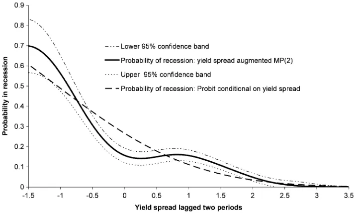
Figure1plots the probability of a recession given the spread, i.e.,E(1−St|spt−2),againstspt−2found in two ways. One is
by estimating a static Probit model and the other is the implied value coming from first fitting the GDC model in Equation (17) to the data and then using Equation (20) to compute the req-uisite expectation. Before doing so, a test was performed on whether the Markov process forSt should be third rather than
second order and the latter was favored. Also shown on the fig-ure are the 95% confidence bands obtained using the asymptotic results for the estimator of 1−E(St|xt)given in Equation (26).
It is clear that there is a difference between the probability of recession obtained from the static Probit and GDC models at a number of values for the spread. Most notably this occurs for
spreads in the range−0.55% to 0.5%, although there is close to being a significant difference for a spread around−1%; at that point, the static Probit model yields a predicted probability of recession that is much lower than the GDC model.
Having established that making an allowance for the nature of St is both theoretically and empirically important, it is of
interest to evaluate the extent to which the yield spread is useful when looking at the probability of moving from an established phase to the opposite one. To assess this we focus on either the probability that an expansion which has lasted for two or more periods will be terminated or the probability of continuing in a contraction that has lasted for two or more periods. The former is the quantityE(St=0|xt,St−1=1,St−2=1),while the latter
isE(St=1|xt,St−1=0,St−2=0).
The probability of leaving an expansion that has lasted for two or more quarters is shown in Figure2. There is a substantial difference between the estimates obtained from the nonpara-metric estimates of the GDC model and those from adynamic Probit model that uses spt−2 andSt−1 as covariates (the
vari-ant used in some of the cycle literature). The dynamic Probit model over-predicts the probability of leaving an expansion for yield spreads in the range−1.1% to 0.3%, and under-predicts the probability of leaving an expansion for yield spreads below −1.1%. These differences are statistically significant at the 5% level for spreads in the interval−0.75% to 0%. The main find-ing that the probability of terminatfind-ing an expansion is low for spreads above−0.75 should be of interest to policy makers.
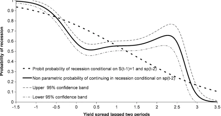
The probability of continuing in a recession that has lasted for two quarters is plotted in Figure3. Again, the probabilities are from the GDC model and the dynamic Probit model. There is a substantial difference between the predicted probabilities from the two models, and this difference is both economically and statistically significant. The most important difference be-tween the probabilities from the two methods is that the GDC model suggests that there is no decrease in the probability of staying in a recession, with a rise in the yield spread from 0% to 2.5%. In contrast, the dynamic Probit model suggests that the
Figure 1. Probability of recession from MP(2) and Probit models conditional on the yield spread lagged two quarters.
92 Journal of Business & Economic Statistics, January 2011
Figure 2. Probability of terminating an expansion that has lasted for two quarters.
probability of remaining in recession declines monotonically as the yield spread increases.
Of course, one may question the accuracy of the asymptotic confidence intervals for this experiment, as there are only 10% of cases where the economy is in contraction for two or more periods. But, even allowing for this caveat, the results presented above are likely to be of considerable practical interest.
6. CONCLUSION
We argue that constructed statesStrequire careful treatment
if they are to be used in econometric work, since they are very different in their nature to the binary states often modeled in microeconometrics. When engaging in a broad range of esti-mation and inference methods one has to allow for the fact that they are essentially Markov processes. But, to date, the nature of theSt has mostly been ignored, with the potential for
mis-leading estimates and inferences. We suggest some methods to deal with this fact. In the application, these methods produce
results that differ from those obtained by a standard Probit pro-cedure that does not allow for the Markov-process nature of the binary states and which forces a particular functional form upon the data. We show that these differences are economically and statistically significant.
APPENDIX A: OBTAINING TRANSITION PROBABILITIES UNDER THE
“TWO QUARTERS RULE”
The task of obtaining transition probabilities becomes much more complex with the “two quarters rule” as the condition-ing eventSt−1=1 will place some restrictions upon the past
sample paths for{yt}that can be associated with the
transi-tion from an expansion to contractransi-tion. In this appendix we first set out a procedure for enumerating sample paths that are con-sistent withSt−1=1. We then apply that procedure to obtain
the univariate transition probabilities whenytfollows a random
walk with drift. We first investigate the case where the drift is
Figure 3. Probability of continuing in a recession.
a constant and then study the case where the drift is a function of some exogenous random variablext. With the “two quarters”
rule the key feature of the sample path is whetheryt is
posi-tive or negaposi-tive. We use “+t” to denote the former and “−t” to
denote the latter.
Enumerating Sample Paths
To formalize the discussion it is helpful to separate the set of paths that are consistent withSt−1=1 into two subsets. Let
Et be the set of paths such that{yt>0 and St−1=1} and
Ft be the set of paths such that{yt<0 andSt−1=1}.If we
introduce the notation that
• [+−]jt represents the fragment of the path along which
there arej repetitions of the pattern[+−] with the lead-ing term in the pattern belead-ing located at timet,
• [++]t represents the fragment of path where the pattern
“++” occurs with the first “+” being attand the second
a shift from the expansion to the contraction phase. This will involve the setGt+1that is enumerated as
Gt+1=
A longer discussion of the issues in enumerating sample paths is in the appendix to the working paper version of this article (Harding and Pagan2009).
Transition Probabilities Whenyt Is a Gaussian Random
Walk With Constant Drift
Hereyt=μ+σet, whereet∼N(0,1)andψt≡Pr(yt≤
0)=(−σμ), where(·)is the cdf of the standard normal. Thus, using the notation that Pr(Et)represents the probability
that the path is drawn from the setEt, and recognizing that the
setsEtandFtare mutually exclusive, we have,
Pr(Et)=
Combining the above results, the probability of transiting from expansion to contractionp10≡Pr(St=0|St−1=1)is defined
The assumption thatytis a random walk with constant drift
and variance implies that
The probabilities that the economy stays in the same state, i.e.,p00andp11are found from the identities
1=p10+p11 (A.14)
94 Journal of Business & Economic Statistics, January 2011
Finally, the transition probabilities can be combined into the following first-order equation
St=p01+ [p11+p01]St−1+νt. (A.18)
Transition Probabilities Whenyt Is a Random Walk With
Time Varying Drift
Now in some of the literature we deal with, it is assumed that the process foryt depends linearly upon some other variable xtin the following way:
yt=a+bxt+εt, (A.19)
where thext are taken to be strictly exogenous (and so can be
conditioned upon) andεtisnid(0,1).It will be convenient to let
pass all of the paths along whichSt=1 under the two quarters
rule. Thus,
Pr(St=1|ℑt+1)=Pr(Et+1|ℑt+1)+Pr(Ft+1|ℑt+1). (A.22)
It is clear from this expression that the use of the two quarters dating rule means that Pr(St=1|ℑt+1)is a function not only of
only. Moreover, the mapping betweenStandxtwill not be that
from the cdf of a standard normal, as assumed in Probit mod-els. Clearly the lesson of this analysis is that one cannot assume either the form of Pr(St=1|ℑt)or that it depends on only a
con-temporaneous variablext; it is necessary that one know how the Stwere generated in order to be able to write down the correct
likelihood.
ACKNOWLEDGMENTS
The authors thank the editor, a referee, an associate editor, and Mardi Dungey for constructive comments on an earlier ver-sion of the article. Pagan acknowledges support from by ESRC grant 000 23-0244 and ARC grant LP0669280. Harding ac-knowledges support from a Latrobe FLM large grant.
[Received January 2008. Revised July 2009.]
REFERENCES
Bierens, H. J. (1983), “Uniform Consistency of Kernel Estimators of a Re-gression Function Under Generalized Conditions,”Journal of the American Statistical Association, 77, 699–707. [90]
Bordo, M. D., and Wheelock, D. C. (2006), “When Do Stock Market Booms Occur? The Macroeconomic and Policy Environments of 20th Century Booms,” Working Paper 2006-051A, Federal Reserve Bank of St. Louis. [88]
Bry, G., and Boschan, C. (1971),Cyclical Analysis of Time Series: Selected Procedures and Computer Programs, New York: NBER. [87,88] Cashin, P., and McDermott, C. J. (2002), “Riding on the Sheep’s Back:
Ex-amining Australia’s Dependence on Wool Exports,”Economic Record, 78, 249–263. [87]
Claessens, S., Kose, M. A., and Terrones, M. E. (2008), “What Happens Dur-ing Recessions: Crunches and Busts,” WorkDur-ing Paper 08/274, International Monetary Fund. [88]
de Jong, R., and Woutersen, T. (2010), “Dynamic Time Series Binary Choice,” Econometric Theory, to appear. [87]
Eichengreen, B., Rose, A. K., and Wyplosz, C. (1995), “Exchange Rate May-hem: The Antecedents and Aftermath of Speculative Attacks,”Economic Policy, 21, 251–312. [88]
Eichengreen, B., Watson, M. W., and Watson, R. S. (1985), “Bank Rate Policy Under the Interwar Gold Standard: A Dynamic Probit Model,”The Eco-nomic Journal, 95, 725–745. [86]
Estrella, A., and Mishkin, F. S. (1998), “Predicting US Recessions: Finan-cial Variables as Leading Indicators,”Review of Economics and Statistics, LXXX, 28–61. [87,91]
Hamilton, J. D. (1989), “A New Approach to the Economic Analysis of Non-Stationary Times Series and the Business Cycle,”Econometrica, 57, 357– 384. [87]
Harding D., and Pagan, A. R. (2002), “Dissecting the Cycle: A Methodological Investigation,”Journal of Monetary Economics, 49, 365–381. [87]
(2006), “Synchronization of Cycles,”Journal of Econometrics, 132, 59–79. [86]
(2009), “An Econometric Analysis of Some Models for Constructed Binary Time Series,” Working Paper 39, NCER. [93]
Ibbotson, R. G., and Jaffee, J. J. (1975), “‘Hot Issue’ Markets,”Journal of Fi-nance, 30, 1027–1042. [88]
Kauppi, H., and Saikkonen, P. (2008), “Predicting U.S. Recessions With Dy-namic Binary Response Models,”Review of Economics and Statistics, 90, 777–791. [87]
Kedem, B. (1980),Binary Time Series, New York: Marcel Dekker. [86,87] Li, Q., and Racine, J. S. (2007), Nonparametric Econometrics, Princeton:
Princeton University Press. [90]
Lunde, A., and Timmermann, A. (2004), “Duration Dependence in Stock Prices: An Analysis of Bull and Bear Markets,”Journal of Business & Eco-nomic Statistics, 22, 253–273. [88]
Meyn, S. (2007),Control Techniques for Complex Networks, Cambridge: Cam-bridge University Press. [88]
Neftci, S. N. (1984), “Are Economic Times Series Asymmetric Over the Busi-ness Cycle,”Journal of Political Economy, 92, 307–328. [87]
Newey, W. K., and West, K. D. (1987), “A Simple Positive Semi-Definite, Het-eroskedasticity and Autocorrelation Consistent Covariance Matrix,” Econo-metrica, 55, 703–708. [86]
Pagan, A. R., and Sossounov, K. (2003), “A Simple Framework for Analyzing Bull and Bear Markets,”Journal of Applied Econometrics, 18, 23–46. [88] Racine, J. S., and Li, Q. (2004), “Non-Parametric Estimation of Regression
Functions,”Journal of Applied Econometrics, 119, 99–130. [90]
Robinson, P. M. (1983), “Nonparametric Estimators for Time Series,”Journal of Time Series Analysis, 4, 185–207. [90]
Startz, R. (2008), “Binomial Autoregressive Moving Average Models With an Application to U.S. Recessions,”Journal of Business & Economic Statis-tics, 26, 1–8. [86,88]
Watson, M. W. (1994), “Business Cycle Durations and Postwar Stabilization of the U.S. Economy,”American Economic Review, 84, 24–46. [86]