Full Terms & Conditions of access and use can be found at
http://www.tandfonline.com/action/journalInformation?journalCode=ubes20
Download by: [Universitas Maritim Raja Ali Haji] Date: 12 January 2016, At: 17:31
Journal of Business & Economic Statistics
ISSN: 0735-0015 (Print) 1537-2707 (Online) Journal homepage: http://www.tandfonline.com/loi/ubes20
Real-Time Measurement of Business Conditions
S. Borağan Aruoba, Francis X. Diebold & Chiara Scotti
To cite this article: S. Borağan Aruoba, Francis X. Diebold & Chiara Scotti (2009) Real-Time Measurement of Business Conditions, Journal of Business & Economic Statistics, 27:4, 417-427, DOI: 10.1198/jbes.2009.07205
To link to this article: http://dx.doi.org/10.1198/jbes.2009.07205
Published online: 01 Jan 2012.
Submit your article to this journal
Article views: 1980
View related articles
Real-Time Measurement of Business Conditions
S. Bora ˘gan A
RUOBADepartment of Economics, University of Maryland, College Park, MD 20742 (aruoba@econ.umd.edu)
Francis X. D
IEBOLDDepartments of Economics, Finance and Statistics, University of Pennsylvania, Philadelphia, PA 19104 and NBER (fdiebold@sas.upenn.edu)
Chiara S
COTTIBoard of Governors of the Federal Reserve System, Washington, DC 20551 (chiara.scotti@frb.gov) We construct a framework for measuring economic activity at high frequency, potentially in real time. We use a variety of stock and flow data observed at mixed frequencies (including very high frequencies), and we use a dynamic factor model that permits exact filtering. We illustrate the framework in a prototype empirical example and a simulation study calibrated to the example.
KEY WORDS: Business cycle; Contraction; Dynamic factor model; Expansion; Macroeconomic fore-casting; Recession; State space model; Turning point.
1. INTRODUCTION
Aggregate business conditions are of central importance in the business, finance, and policy communities worldwide, and huge resources are devoted to assessment of the continuously evolving state of the real economy. Literally thousands of news-papers, newsletters, television shows, and blogs, not to mention armies of employees in manufacturing and service industries, including the financial services industries, central banks, gov-ernment, and nongovernment organizations, grapple constantly with the measurement and forecasting of evolving business con-ditions. Of central importance is theconstantgrappling. Real economic agents, making real decisions, in real time, want ac-curate andtimelyestimates of the state of real activity. Business cycle chronologies such as the NBER’s, which proclaim expan-sions and contractions long after the fact, are not useful in that regard.
Against this background, we propose and illustrate a frame-work for high-frequency business conditions assessment in a systematic, replicable, and statistically optimal manner. Our framework has four key ingredients.
Ingredient1. We work with a dynamic factor model, treat-ing business conditions as an unobserved variable, related to observed indicators.Latency of business conditions is consis-tent with economic theory (e.g., Lucas1977), which empha-sizes that the business cycle is not about any single variable, whether GDP, industrial production, sales, employment, or any-thing else. Rather, the business cycle is about the dynamics and interactions (“comovements”) of many variables.
Treating business conditions as latent is also a venerable tra-dition in empirical business cycle analysis, ranging from the earliest work to the most recent, and from the statistically in-formal to the statistically in-formal. On the inin-formal side, latency of business conditions is central to many approaches, from the classic early work of Burns and Mitchell (1946) to the recent workings of the NBER business cycle dating committee, as de-scribed, for example by Hall et al. (2003). On the formal side, latency of business conditions is central to the popular dynamic factor framework, whether from the “small data” perspective of
Geweke (1977), Sargent and Sims (1977), Stock and Watson (1989,1991), and Diebold and Rudebusch (1996), or the more recent “large data” perspective of Forni et al. (2000), Stock and Watson (2002), and Bai and Ng (2006). (For discussion of small-data versus large-data dynamic factor modeling, see Diebold2003.)
Ingredient 2. We explicitly incorporate business conditions indicators measured at different frequencies. Important busi-ness conditions indicators do in fact arrive at a variety of fre-quencies, including quarterly (e.g., GDP), monthly (e.g., indus-trial production), weekly (e.g., employment), and continuously (e.g., asset prices), and we want to be able to incorporate all of them, to provide continuously updated measurements.
Ingredient3.We explicitly incorporate indicators measured at high frequencies. Given that our goal is to track the high-frequency evolution of real activity, it is important to incorpo-rate (or at least not exclude from the outset) the high-frequency information flow associated with high-frequency indicators.
Ingredient4.We extract and forecast latent business condi-tions using linear yet statistically optimal procedures, which in-volve no approximations. The appeal of exact as opposed to ap-proximate procedures is obvious, but achieving exact optimality is not trivial, due to complications arising from temporal aggre-gation of stocks versus flows in systems with mixed-frequency data.
Related to our concerns and framework is a small but never-theless important literature, including Stock and Watson (1989, 1991), Mariano and Murasawa (2003), Evans (2005), and Proi-etti and Moauro (2006), as well as Shen (1996), Abeysinghe (2000), Altissimo et al. (2001), Liu and Hall (2001), McGuckin, Ozyildirim, and Zarnowitz (2003), Ghysels et al. (2004), and Giannone, Reichlin, and Small (2008).
Our contribution is different in certain respects, and similar in others, and both the differences and similarities are inten-tional. Let us begin by highlighting some of the differences.
© 2009American Statistical Association Journal of Business & Economic Statistics
October 2009, Vol. 27, No. 4 DOI:10.1198/jbes.2009.07205
417
First, some authors like Stock and Watson (1989,1991) work in a dynamic factor framework with exact linear filtering, but they do not consider data at mixed frequencies or at high fre-quencies.
Second, other authors like Evans (2005) do not use a dynamic factor framework and do not use high-frequency data, instead focusing on estimating high-frequency GDP. Evans (2005), for example, equates business conditions with GDP growth and uses state space methods to estimate daily GDP growth using data on preliminary, advanced, and final releases of GDP and other macroeconomic variables.
Third, authors like Mariano and Murasawa (2003) work in a dynamic factor framework and consider data at mixed fre-quencies, but not high frefre-quencies, and their filtering algo-rithm is only approximate. Proietti and Moauro (2006) avoid the Mariano–Murasawa approximation at the cost of moving to a nonlinear model with a corresponding rather tedious nonlin-ear filtering algorithm.
Ultimately, however, thesimilaritiesbetween our work and others’ are more important than the differences, as we stand on the shoulders of many earlier authors. Effectively we (1) take a small-data dynamic factor approach to business conditions analysis, (2) recognize the potential practical value of extending the approach to mixed-frequency data settings involving some high-frequency data, (3) recognize that doing so amounts to a filtering problem with a large amount of missing data, which the Kalman filter is optimally designed to handle, and (4) pro-vide a prototype example of the framework in use. Hence the paper is really a “call to action,” a call to move the state-space dynamic-factor framework closer to its high-frequency limit, and hence to move statistically rigorous business conditions analysis closer toitshigh-frequency limit.
We proceed as follows. In Section2 we provide a detailed statement of our dynamic-factor modeling framework, and in Section 3 we represent it as a state-space filtering problem with a large amount of missing data. In Section 4 we report the results of a four-indicator prototype empirical analysis, us-ing quarterly GDP, monthly employment, weekly initial jobless claims, and the daily yield curve term premium. We also report the results of a simulation exercise, calibrated to our empirical estimates, which lets us illustrate our methods and assess their efficacy in a controlled environment. In Section5we conclude and offer directions for future research.
2. THE MODELING FRAMEWORK
Here we propose a dynamic factor model at daily frequency. The model is very simple at daily frequency, but of course the daily data are generally not observed, so most of the data are missing. Hence we explicitly treat missing data and temporal aggregation, and we obtain the measurement equations for ob-served stock and flow variables. Following that, we enrich the model by allowing for lagged state variables in the measure-ment equations, and by allowing for trend, both of which are important when fitting the model to macroeconomic and finan-cial indicators.
2.1 The Dynamic Factor Model at Daily Frequency
We assume that the state of the economy evolves at a very high frequency; without loss of generality, call it “daily.” In our subsequent empirical work, we will indeed use a daily base observational frequency, but much higher (intraday) frequen-cies could be used if desired. Economic and financial variables, although evolving daily, are of course not generallyobserved
daily. For example, an end-of-year wealth variable is observed each December 31, and is unobserved every other day of the year.
Letxt denote underlying business conditions at dayt, which
evolve daily withAR(p)dynamics,
xt=ρ1xt−1+ρ2xt−2+ · · · +ρpxt−p+et, (1)
whereetis a white noise innovation with unit variance. We are
interested in tracking and forecasting real activity, so we use a single-factor model; that is,xt is a scalar, as, for example,
in Stock and Watson (1989). Additional factors could be intro-duced to track, for example, wage/price developments.
Letyit denote theith daily economic or financial variable at dayt, which depends linearly onxtand possibly also on various
exogenous variables and/or lags ofyit:
yit=ci+βixt+δi1w1t + · · · +δikwkt
+γi1yit−Di+ · · · +γiny
i
t−nDi+u
i t, (2)
where thewt are exogenous variables and theuit are
contem-poraneously and serially uncorrelated innovations. Notice that we introduce lags of the dependent variableyit in multiples of
Di, whereDi>1 is a number linked to the frequency of the
observedyit. (We will discussDi in detail in the next
subsec-tion.) Modeling persistence only at the daily frequency would be inadequate, as it would decay too quickly.
2.2 Missing Data, Stocks versus Flows, and Temporal Aggregation
Recall thatyit denotes theith variable on a daily time scale. But most variables, althoughevolvingdaily, are not actually ob-serveddaily. Hence lety˜itdenote the same variable observed at a lower frequency (call it the “tilde frequency”). The relationship between˜yitandyitdepends crucially on whetheryitis a stock or flow variable.
If yit is a stock variable measured at a nondaily tilde fre-quency, then the appropriate treatment is straighforward, be-cause stock variables are simply point-in-time snapshots. At any timet, either yit is observed, in which case y˜it=yit, or it
is not, in which casey˜i
t=NA, whereNAdenotes missing data
(“not available”). Hence we have the stock variable measure-ment equation:
˜
yit=
⎧ ⎪ ⎪ ⎨
⎪ ⎪ ⎩
yit=ci+βixt+δi1w1t + · · · +δikwkt
+γi1yit−Di+ · · · +γiny
i
t−nDi+u
i t
ifyitis observed
NA otherwise.
(3)
Now consider flow variables. Flow variables observed at nondaily tilde frequencies are intraperiod sums of the corre-sponding daily values,
whereDiis the number of days per observational period (e.g.,
Di=7 if yit is measured weekly). Combining this fact with
Equation (2), we arrive at the flow variable measurement equa-tion
t−Di−jis by definition the observed flow variable one period ago (y˜it−D
i), andu
∗i
t is the sum of theuitover the tilde
period.
Discussion of two subtleties is in order. First, note that in generalDiis time varying, as, for example, some months have
28 days, some have 29, some have 30, and some have 31. To simplify the notation above, we ignored this, implicitly assum-ing thatDi is fixed. In our subsequent empirical
implementa-tion, however, we allow for time-varyingDi.
Second, note that although u∗ti follows a moving average process of orderDi−1 at the daily frequency, it nevertheless
remains white noise when observed at the tilde frequency, due to the(Di−1)-dependence of anMA(Di−1)process. Hence
we appropriately treatu∗tias white noise in what follows, where var(u∗ti)=Di·var(uit).
2.3 Trend
The exogenous variableswtare the key to handling trend. In
particular, in the important special case where thewtare simply
deterministic polynomial trend terms [w1t−j=t−j,w2t−j=(t− In theAppendixwe derive the mapping between the “starred” and “unstarred”c’s and δ’s for cubic trends, which are suffi-ciently flexible for most macroeconomic data and of course in-clude linear and quadratic trends as special cases. Assembling
the results, we have the stock variable measurement equation
˜
and the flow variable measurement equation,
˜
This completes the specification of our model, which has a natural state-space form, to which we now turn.
3. STATE–SPACE REPRESENTATION, SIGNAL EXTRACTION, AND ESTIMATION
Here we discuss our model from a state-space perspective, in-cluding filtering and estimation. We avoid dwelling on standard issues, focusing instead on the nuances specific to our frame-work, including missing data due to mixed-frequency mod-eling, high-dimensional state vectors due to the presence of flow variables, and time-varying system matrices due to varying lengths of months.
3.1 State-Space Representation
Our model is trivially cast in state-space form as
yt=Ztαt+Ŵtwt+εt, (9)
αt+1=Tαt+Rηt, (10)
εt∼(0,Ht), ηt∼(0,Q), (11)
t=1, . . . ,T,
whereyt is anN×1 vector of observed variables (subject, of
course, to missing observations),αtis anm×1 vector of state
variables,wtis ae×1 vector of predetermined variables
con-taining a constant term (unity),ktrend terms andN×nlagged dependent variables (nfor each of theNelements of theyt
vec-tor),εtandηtare vectors of measurement and transition shocks
containing theuitandet, andT denotes the last time-series
ob-servation.
In general, the observed vectorytwill have a very large
num-ber of missing values, reflecting not only missing daily data due to holidays, but also, and much more importantly, the fact that most variables are observed much less often than daily. Interest-ingly, the missing dataper sedoes not pose severe challenges:
ytis simply littered with a large number ofNAvalues, and the
corresponding system matrices are very sparse, but the Kalman filter remains valid (appropriately modified, as we discuss be-low), and numerical implementations may indeed be tuned to exploit the sparseness, as we do in our implementation.
In contrast, the presence of flow variables produces more sig-nificant complications, and it is hard to imagine a serious busi-ness conditions indicator system without flow variables, given
that real output is itself a flow variable. Flow variables pro-duce intrinsically high-dimensional state vectors. In particu-lar, as shown in Equation (3), the flow variable measurement equation contains xt and maxi{Di} −1 lags of xt, producing
a state vector of dimension max{maxi{Di},p}, in contrast to
thep-dimensional state associated with a system involving only stock variables. In realistic systems with data frequencies rang-ing from, say, daily to quarterly, maxi{Di} ≈90.
There is a final nuance associated with our state-space sys-tem: several of the system matrices are time varying. In partic-ular, althoughT,R, andQare constant,Zt,Ŵt, andHtare not,
because of the variation in the number of days across quarters and months (i.e., the variation inDiacrosst). Nevertheless the
Kalman filter remains valid.
3.2 Signal Extraction
With the model cast in state-space form, and for given para-meters, we use the Kalman filter and smoother to obtain opti-mal extractions of the latent state of real activity. As is standard for classical estimation, we initialize the Kalman filter using the unconditional mean and covariance matrix of the state vec-tor. We use the contemporaneous Kalman filter; see Durbin and Koopman (2001) for details.
LetYt≡ {y1, . . . ,yt},at|t≡E(αt|Yt),Pt|t=var(αt|Yt),at≡
E(αt|Yt−1), andPt=var(αt|Yt−1). Then the Kalman filter
up-dating and prediction equations are
at|t=at+PtZ′tF
−1
t vt, (12)
Pt|t=Pt−PtZ′tF
−1
t ZtP′t, (13)
at+1=Tat|t, (14)
Pt+1=TPt|tT′+RQR′, (15)
where
vt=yt−Ztat−Ŵtwt, (16)
Ft=ZtPtZ′t+Ht (17)
fort=1, . . . ,T.
Crucially for us, the Kalman filter remains valid with missing data. If all elements ofytare missing, we skip updating and the
recursion becomes
at+1=Tat, (18)
Pt+1=TPtT′+RQR′. (19)
If some but not all elements ofyt are missing, we replace the
measurement equation with
y∗t =Z∗tαt+Ŵ∗twt+ε∗t, (20)
ε∗t ∼N(0,H∗t), (21) wherey∗t is of dimensionN∗<N, containing the elements of theytvector that are observed. The key insight is thaty∗t andyt
are linked by the transformationy∗t =Wtyt, whereWtis a
ma-trix whoseN∗rows are the rows ofINcorresponding to the
ob-served elements ofyt. Similarly,Z∗t =WtZt,Ŵ∗t =WtŴt,ε∗t =
Wtεt, andH∗t =WtHtW′t. The Kalman filter works exactly as
described above, replacingyt,Zt, andHtwithy∗t,Z∗t, andH∗t.
Similarly, after transformation the Kalman smoother remains valid with missing data.
3.3 Estimation
Thus far we have assumed known system parameters, where-as they are of course unknown in practice. As is well known, however, the Kalman filter supplies all of the ingredients needed for evaluating the Gaussian pseudo log-likelihood function via the prediction error decomposition,
logL= −1
2 T
t=1
Nlog 2π+(log|Ft| +v′tF
−1
t vt). (22)
In calculating the log likelihood, if all elements ofyt are
miss-ing, the contribution of periodtto the likelihood is zero. When some elements ofyt are observed, the contribution of periodt
is[N∗log 2π+(log|F∗t| +vt∗′F∗−t 1v∗t)]whereN∗is the number of observed variables, and we obtainF∗t andv∗t by filtering the transformedy∗t system.
4. A PROTOTYPE EMPIRICAL APPLICATION
We now present a simple application involving the daily term premium, weekly initial jobless claims, monthly employment, and quarterly GDP. We describe in turn the data, the specific variant of the model that we implement, subtleties of our esti-mation procedure, and our empirical results.
4.1 Business Conditions Indicators
Our analysis covers the period from April 1, 1962 through February 20, 2007, which is 16,397 observations of daily data. (We use a seven-day week.)
We use four indicators. Moving from highest frequency to lowest frequency, the first indicator is the yield curve term pre-mium, defined as the difference between 10-year and 3-month U.S. Treasury yields. We measure the term premium daily; hence there are no aggregation issues. We treat holidays and weekends as missing.
The second indicator is initial claims for unemployment in-surance, a weekly flow variable covering the seven-day period from Sunday to Saturday. We set the Saturday value to the sum of the previous seven daily values, and we treat other days as missing.
The third indicator is employees on nonagricultural payrolls, a monthly stock variable. We set the end-of-month value to the end-of-month daily value, and we treat other days as missing.
The fourth and final indicator is real GDP, a quarterly flow variable. We set the end-of-quarter value to the sum of daily values within the quarter, and we treat other days as missing.
Several considerations guide our choice of variables. First, we want the variables chosen to illustrate the flexibility of our framework. Hence we choose four variables measured at four different frequencies ranging from very high (daily) to very low (quarterly), and representing both stocks (term premium, pay-roll employment) and flows (initial claims, GDP). Second, we want our illustrative analysis to be credible, if not definitive. Al-though reasonable people can (and will) disagree on the number and choice of indicators, our choices are easily defensible. GDP needs no defense. Labor market variables like payroll employ-ment and initial claims are strongly cyclical and feature promi-nently in many coincident indexes. The Conference Board’s
composite coincident index, for example, also uses payroll em-ployment. Finally, the term premium is also strongly cyclical, as studied, for example, in Diebold, Rudebusch, and Aruoba (2006) and several of the papers they cite.
4.2 Model Implementation
In the development thus far we have allowed for general polynomial trend and generalAR(p)dynamics. In the prototype model that we now take to the data, we make two simplifying assumptions that reduce the number of parameters to be esti-mated by numerical likelihood optimization. First, we de-trend prior to fitting the model rather than estimating trend parame-ters simultaneously with the others, and second, we use simple first-order dynamics throughout. In future work we look for-ward to incorporating more flexible dynamics but, as we show below, the framework appears quite encouraging even with sim-pleAR(1)dynamics.
Hence, latent business conditionsxtfollow zero-meanAR(1)
process, as do the observed variables at their observational fre-quencies. For weekly initial claims, monthly employment, and quarterly GDP, this simply means that the lagged values of these variables are elements of the wt vector. We denote these by
˜
y2t−W,y˜3t−M, andy˜4t−q, whereWdenotes the number of days in a week,Mdenotes the number of days in a month andqdenotes the number of days in a quarter. (Once again, the notation in the paper assumesM andqare constant over time, but in the im-plementation we adjust them according to the number of days in the relevant month or quarter.)
For the term premium, on the other hand, we model the au-tocorrelation structure using anAR(1)process for the measure-ment equation innovation,u1t, instead of adding a lag of the term premium inwt.
The equations that define the model are
⎡
where the notation corresponds to the system in Section3with
N=4, k=3,m=93,p=1, and r=2. We use the current factor and 91 lags in our state vector because the maximum possible number of days in a quarter is 92, which we denote byq¯. (If there areqdays in a quarter, then on the last day of the quarter we need the current value andq−1 lags.) Also, in every quarter we adjust the number of nonzero elements in the fourth row of theZtmatrix to reflect the number of days in that
quarter.
4.3 Estimation
The size of our estimation problem is substantial. We have 16,397 daily observations, and even with de-trended data and first-order dynamics we have 93 state variables and 13 coeffi-cients. Using a Kalman filter routine programmed in MATLAB, one evaluation of the likelihood takes about 20 seconds. Max-imization of the likelihood, however, may involve a very large number of likelihood evaluations, so it’s crucial to explore the parameter space in a sophisticated way. Throughout, we use a quasi-Newton algorithm with BFGS updating of the inverse Hessian, using accurate start-up values for iteration. [Perhaps the methods of Jungbacker and Koopman (2008) could be used to improve the speed of our gradient evaluation, although we have not yet explored that avenue. Our real problem is the huge sample size.]
We obtain our start-up values in two steps, as follows. In the first step, we use only daily and stock variables, which drasti-cally reduce the dimension of the state vector, resulting in very fast estimation. This yields preliminary estimates of all mea-surement equation parameters for the daily and stock variables, and all transition equation parameters, as well as a preliminary extraction of the factor,xˆt(via a pass of the Kalman smoother).
In the second step, we use the results of the first step to obtain start-up values for the remaining parameters, that is, those in the flow variable measurement equations. We simply regress the flow variables on the smoothed state extracted in the first step and take the coefficients as our start-up values.
Obviously in the model that we use in this paper, the vari-ables that we use in the first step are the daily term premium and monthly employment, and the variables that we use in the second step are weekly initial claims and quarterly GDP. (Note that the same simple two-step method could be applied equally easily in much larger models.) At the conclusion of the second step we have start-up values for all parameters, and we proceed to estimate the full model’s parameters jointly, after which we obtain our “final” extraction of the latent factor.
4.4 Results
Here we discuss a variety of aspects of our empirical re-sults. To facilitate the discussion, we first define some nomen-clature to help us distinguish among models. We call our full four-variable model GEIS (“GDP, Employment, Initial Claims, Slope”). Similarly, proceeding to drop progressively more of the high-frequency indicators, we might consider GEI or GE models.
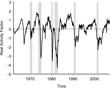
4.4.1 The Smoothed GEIS Real Activity Indicator. We start with our centerpiece, the extracted real activity indicator (factor). In Figure 1 we plot the smoothed GEIS factor with NBER recessions shaded. (Because the NBER provides only months of the turning points, we assume recessions start on the first day of the month and end on the last day of the month.)
Several observations are in order. First, our real activity in-dicator broadly coheres with the NBER chronology. There are, for example, no NBER recessions that are not also reflected in our indicator. Of course there is nothing sacred about the NBER chronology, but it nevertheless seems comforting that the two cohere. The single broad divergence is the mid 1960s episode, which the NBER views as a growth slowdown but we would view as a recession.
Second, if our real activity indicator broadly coheres with the NBER chronology, it nevertheless differs somewhat. In partic-ular, it tends to indicate earlier turning points, especially peaks.
Figure 1. Smoothed real activity factor, full model (GEIS).
That is, when entering recessions our indicator tends to reach its peak and start falling several weeks before the correspond-ing NBER peak. Similarly, when emergcorrespond-ing from recessions, our indicator tends to reach its trough and start rising before the cor-responding NBER trough. In the last two recessions, however, our indicator matches the NBER trough very closely.
One can interpret our indicator’s tendency toward earlier-than-NBER peaks in at least two ways. The NBER chronol-ogy may of course simply be inferior, tending to lag turning points whereas ours does not. Alternatively, the NBER chronol-ogy may be accurate whereas our index may actually have some lead, particularly as one of our component indicators is the daily term premium, which is not only cyclical but may actually lead the cycle (e.g., Diebold, Rudebusch, and Aruoba2006).
Third, our real activity indicator makes clear that there are important differences in entering and exiting recessions, whereas the “0–1” NBER recession indicator cannot. In par-ticular, our indicator consistently plunges at the onset of reces-sions, whereas its growth when exiting recessions is sometimes brisk (e.g., 1973–1975, 1982) and sometimes anemic (e.g., the well-known “jobless recoveries” of 1990–1991 and 2001).
Fourth, and of crucial importance, our indicator is of course available at high frequency, whereas the NBER chronology is available only monthly and withverylong lags (often several years). Hence our indicator is a useful “nowcast,” whereas the NBER chronology is not.
4.4.2 Gains From High-Frequency Data I: Comparison of GE and GEI Factors. Typically, analyses similar to ours are done using monthly and/or quarterly data, as would be the case in a two-variable GE (GDP, employment) model. To see what is gained by inclusion of higher-frequency data, we now compare the real activity factors extracted from a GE model and a GEI model (which incorporates weekly initial claims).
In Figure 2 we show the smoothed GEI factor, and for comparison we show a shaded interval corresponding to the smoothed GE factor±1 SE. The GEI factor is quite different, often violating the±1 SE band, and indeed not infrequently violating a±2 SE band (not shown) as well.
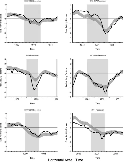
In Figure 3 we dig deeper, focusing on the times around the six NBER recessions: December 1969–November 1970,
Figure 2. Smoothed real activity factors: GE (interval) and GEI (point).
Figure 3. Smoothed real activity factor around NBER recessions GE (interval) and GEI (point).
November 1973–March 1975, January 1980–July 1980, July 1981–November 1982, July 1990–March 1991, and March 2001–November 2001. We consider windows that start 12 months before peaks and end 12 months after troughs. Within each window, we again show the smoothed GEI factor and a shaded interval corresponding to the smoothed GE factor
±1 SE. Large differences are apparent.
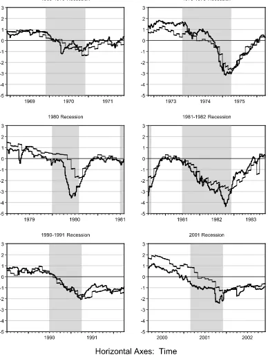
In Figure4we move from smoothed to filtered real activity factors, again highlighting the six NBER recessions. The fil-tered version is the one relevant in real time, and it highlights
another key contribution of the high-frequency information em-bedded in the GEI factor. In particular, the filtered GEI factor evolves quite smoothly with the weekly information on which it is in part based, whereas the filtered GE factor has much more of a discontinuous “step function” look. Looking at the factors closely, the GE factor jumps at the end of every month and then reverts towards to mean (of zero) while the GEI factor jumps every week with the arrival of new Initial Claims data.
Finally, what of a comparison between the GEI factor and the GEIS factor, which incorporates the daily term structure
Figure 4. Filtered real activity factors around NBER recessions GE (thin) and GEI (thick).
slope? In this instance it turns out that, although incorporat-ing weekly data (movincorporat-ing from GE to GEI) was evidently very helpful, incorporating daily data (moving from GEI to GEIS) was not. That is, the GEI and GEIS factors are almost identical. It is important to note, however, that we still need a daily state-space setup even though the highest-frequency data of value were weekly, to accommodate the variation in weeks per month and weeks per quarter.
4.4.3 Gains From High-Frequency Data II: A Calibrated Simulation. Here we illustrate our methods in a simulation calibrated to the empirical results above. This allows us to as-sess the efficacy of our framework in a controlled environment.
In particular, in a simulation we know the true factor, so we can immediately determine whether and how much we gain by in-corporating high-frequency data, in terms of reduced factor ex-traction error. In contrast, in empirical work such as that above, although we can see that the extracted GE and GEI factors dif-fer, we cannot be certain that the GEI factor extraction is more accurate, because we can never see the true factor, even ex post. In our simulation we use the system and the parameters esti-mated previously. Using those parameters, we generate 40 years of “daily” data on all four variables, and then we transform them to obtain the observed data. Specifically, we delete the weekends from the daily variable and aggregate the daily
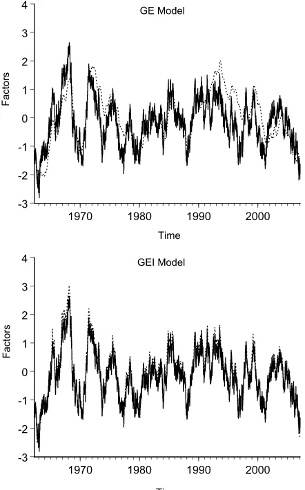
Figure 5. Simulated real activity factors smoothed (dashed) and true (solid).
servations over the week to obtain the observed weekly (flow) variable. We also delete all the observations for the third (stock) variable except for the end-of-the-month observations and sum the daily observations over the quarter to get the fourth (flow) variable. Finally, using the simulated data we estimate the coef-ficients and extract the factor, precisely as we did with the real data.
In the top panel of Figure5we show the true factor together with the smoothed factor from the GE model. The two are of course related, but they often diverge noticeably and system-atically, for long periods. The correlation between the two is 0.72 and the mean squared extraction error is 0.45. In the bot-tom panel of Figure5we show the true factor together with the smoothed factor from the GEI model. The two are much more closely related and indeed hard to distinguish. The correlation between the two is 0.98 and the mean squared extraction error is 0.07. This exercise quite convincingly shows that incorporat-ing high-frequency data improves the accuracy of the extracted factor.
4.4.4 Real-Time Performance. At any point T in real time, we simply use the time-T data vintage to extract the real activity factor at timeT and earlier, as in Corradi, Fernandez, and Swanson (2007). As time progresses, we reestimate the sys-tem each period (or less frequently if desired for convenience),
Figure 6. Tentacle plot: six real activity paths assessed in 2008.
always using the latest-vintage data to extract the real activity factor.
In Figure6we show what we call a “tentacle plot” for part of 2008, that is, a plot of several series of real activity factors extracted using sequential vintages of 2008 data. The tentacle plot contains six paths, extracted on April 4, June 12, June 28, July 19, August 9, and August 30. The six paths show clearly that newly arrived data can produce substantial changes in op-timal assessments of real activity. It is interesting to note, for example, that the two assessments using August data vintages produce August values of the real activity factor below the lev-els seen at the onset of both the 1990–1991 and 2001 recessions, but still far from the levels seen at those recessions’ troughs, indicating not only recession, but also that conditions would likely worsen before improving.
5. SUMMARY AND CONCLUDING REMARKS
We view this paper as providing both (1) a “call to action” for measuring macroeconomic activity in real time, using a variety of stock and flow data observed at mixed frequencies, poten-tially also including very high frequencies, and (2) a prototype empirical application, illustrating the gains achieved by moving beyond the customary monthly data frequency. Specifically, we have proposed a dynamic factor model that permits exactly op-timal extraction of the latent state of macroeconomic activity, and we have illustrated it in a four-variable empirical applica-tion with a daily base frequency, and in a parallel calibrated simulation.
We look forward to a variety of variations and extensions of our basic theme, including but not limited to:
(1) Incorporation of indicators beyond macroeconomic and financial data. In particular, it will be of interest to attempt in-clusion of qualitative information such as headline news.
(2) Construction of a real-time composite leading index (CLI). Thus far we have focused only on construction of a com-posite coincident index (CCI), which is the more fundamental problem, because a CLI is simply a forecast of a CCI. Explicit construction of a leading index will nevertheless be of interest.
(3) Allowance for nonlinear regime-switching dynamics. The linear methods used in this paper provide only a partial (linear) statistical distillation of the rich business cycle litera-ture. A more complete approach would incorporate the insight that expansions and contractions may be probabilistically dif-ferent regimes, separated by the “turning points” correspond-ing to peaks and troughs, as emphasized for many decades in the business cycle literature and rigorously embodied Hamil-ton’s (1989) Markov-switching model. Diebold and Rudebusch (1996) and Kim and Nelson (1998) show that the linear and nonlinear traditions can be naturally joined via dynamic fac-tor modeling with a regime-switching facfac-tor. Such an approach could be productively implemented in the present context, par-ticularly if interest centers on turning points, which are intrin-sically well defined only in regime-switching environments.
(4) Comparative assessment of experiences and results from “small data” approaches, such as ours, versus “big data” ap-proaches. Although much professional attention has recently turned to big data approaches, as, for example, in Forni et al. (2000) and Stock and Watson (2002), recent theoretical work by Boivin and Ng (2006) shows that bigger is not necessar-ily better. The matter is ultimately empirical, requiring detailed comparative assessment. It would be of great interest, for ex-ample, to compare results from our approach to those from the Altissimo et al. (2001) EuroCOIN approach, for the same econ-omy and time period. Such comparisons are very difficult, of course, because the “true” state of the economy is never known, even ex post.
(5) Complete real-time analysis, recognizing that at any time T we have not only the time-T data vintage, but also all ear-lier data vintages. That would permit incorporation of the sto-chastic process of data revisions, as was attempted (in different contexts) in early work such as Conrad and Corrado (1979) and Howrey (1984) and recent work such as Aruoba (2008). Doing so in the rich dynamic multivariate environment of this paper is presently infeasible, however, due to the large additional esti-mation burden that it would entail.
(6) Exploration of direct indicators of daily activity, such as debit card transactions data, as in Galbraith and Tkacz (2007).
Indeed, progress is already being made in work done sub-sequently to earlier drafts of this paper, such as Camacho and Perez-Quiros (2008).
APPENDIX: TREND REPRESENTATIONS
Here we provide the mapping between the “unstarred” and “starred”c’s andδ’s in Equation (4) of the text, for cubic poly-nomial trend. Cubic trends are sufficiently flexible for most macroeconomic data and of course include linear and quadratic trend as special cases.
The “unstarred” representation of third-order polynomial trend is
The requisite calulation is tedious but straightforward. The “unstarred” expression can be expanded as
D−1
For helpful guidance we thank the Editor, Associate Edi-tor, and referees, as well as seminar and conference partici-pants at the Board of Governors of the Federal Reserve System, the Federal Reserve Bank of Philadelphia, the European Cen-tral Bank, the University of Pennsylvania, SUNY Albany, SCE Cyprus, and American University. We are especially grateful to David Armstrong, Carlos Capistran, Dean Croushore, Martin Evans, Jon Faust, John Galbraith, Eric Ghysels, Sharon Koz-icki, Steve Kreider, Simon van Norden, Alexi Onatski, Simon Potter, Scott Richard, Frank Schorfheide, Roberto Sella, and
Jonathan Wright. For research support we thank the National Science Foundation and the Real-Time Data Research Center at the Federal Reserve Bank of Philadelphia. The views expressed here are solely those of the authors and do not necessarily re-flect those of the Federal Reserve System.
[Received August 2007. Revised September 2008.]
REFERENCES
Abeysinghe, T. (2000), “Modeling Variables of Different Frequencies,” Inter-national Journal of Forecasting, 16, 117–119.
Altissimo, F., Bassanetti, A., Cristadoro, R., Forni, M., Hallin, M., Lippi, M., Reichlin, L., and Veronese, G. (2001), “EuroCOIN: A Real Time Coinci-dent Indicator of the Euro Area Business Cycle,” Discussion Paper 3108, CEPR.
Aruoba, S. B. (2008), “Data Revisions Are Not Well-Behaved,”Journal of Money, Credit and Banking, 40, 319–340.
Bai, J., and Ng, S. (2006), “Confidence Intervals for Diffusion Index Fore-casts and Inference for Factor-Augmented Regressions,”Econometrica, 74, 1133–1150.
Boivin, J., and Ng, S. (2006), “Are More Data Always Better for Factor Analy-sis?”Journal of Econometrics, 127, 169–194.
Burns, A. F., and Mitchell, W. C. (1946),Measuring Business Cycles, New York: NBER.
Camacho, M., and Perez-Quiros, G. (2008), “Introducing the Euro-STING: Short Term Indicator of Euro Area Growth,” manuscript, Bank of Spain. Conrad, W., and Corrado, C. (1979), “Application of the Kalman Filter to
Re-visions in Monthly Retail Sales Estimates,”Journal of Economic Dynamics and Control, 1, 177–198.
Corradi, V., Fernandez, A., and Swanson, N. R. (2007), “Information in the Re-vision Process of Real-Time Datasets,” manuscript, University of Warwick and Rutgers University.
Diebold, F. X. (2003), “‘Big Data’ Dynamic Factor Models for Macroeconomic Measurement and Forecasting” (discussion of Reichlin and Watson papers), inAdvances in Economics and Econometrics, Eighth World Congress of the Econometric Society, eds. M. Dewatripont, L. P. Hansen, and S. Turnovsky, Cambridge: Cambridge University Press, pp. 115–122.
Diebold, F. X., and Rudebusch, G. (1996), “Measuring Business Cycles: A Modern Perspective,”Review of Economics and Statistics, 78, 67–77. Diebold, F. X., Rudebusch, G. D., and Aruoba, S. B. (2006), “The
Macroecon-omy and the Yield Curve: A Dynamic Latent Factor Approach,”Journal of Econometrics, 131, 309–338.
Durbin, J., and Koopman, S. J. (2001),Time Series Analysis by State Space Methods, Oxford: Oxford University Press.
Evans, M. D. D. (2005), “Where Are We Now?: Real Time Estimates of the Macro Economy,”The International Journal of Central Banking, Septem-ber, 127–175.
Forni, M., Hallin, M., Lippi, M., and Reichlin, L. (2000), “The Generalized Fac-tor Model: Identification and Estimation,”Review of Economics and Statis-tics, 82, 540–554.
Galbraith, J., and Tkacz, G. (2007), “Electronic Transactions as High-Frequen-cy Indicators of Economic Activity,” manuscript, McGill University and Bank of Canada.
Geweke, J. F. (1977), “The Dynamic Factor Analysis of Economic Time Series Models,” inLatent Variables in Socioeconomic Models, eds. D. Aigner and A. Goldberger, Amsterdam: North-Holland, pp. 365–383.
Ghysels, E., Santa-Clara, P., and Valkanov, R. (2004), “The MIDAS Touch: Mixed Data Sampling Regression Models,” manuscript, University of North Carolina.
Giannone, D., Reichlin, L., and Small, D. (2008), “Nowcasting: The Real Time Informational Content of Macroeconomic Data,”Journal of Monetary Eco-nomics, 55, 665–676.
Hall, R., Feldstein, M., Frankel, J., Gordon, R., Romer, C., Romer, D., and Zarnowitz, V. (2003), “The NBER’s Recession Dating Procedure,” available athttp:// www.nber.org/ cycles/ recessions.html.
Hamilton, J. D. (1989), “A New Approach to the Economic Analysis of Nonsta-tionary Time Series and the Business Cycle,”Econometrica, 57, 357–384. Howrey, E. P. (1984), “Data Revision, Reconstruction, and Prediction: An
Ap-plication to Inventory Investment,”Review of Economics and Statistics, 66, 386–393.
Jungbacker, B., and Koopman, S. J. (2008), “Likelihood-Based Analysis of Dy-namic Factor Models,” manuscript, Free University of Amsterdam. Kim, C.-J., and Nelson, C. R. (1998),State Space Models With Regime
Switch-ing: Classical and Gibbs Sampling Approaches With Applications, Cam-bridge, MA: MIT Press.
Liu, H., and Hall, S. G. (2001), “Creating High-Frequency National Accounts With State-Space Modelling: A Monte Carlo Experiment,”Journal of Fore-casting, 20, 441–449.
Lucas, R. E. (1977), “Understanding Business Cycles,”Carnegie-Rochester Conference Series on Public Policy, 5, 7–29.
Mariano, R. S., and Murasawa, Y. (2003), “A New Coincident Index of Busi-ness Cycles Based on Monthly and Quarterly Series,”Journal of Applied Econometrics, 18, 427–443.
McGuckin, R. H., Ozyildirim, A., and Zarnowitz, V. (2003), “A More Timely and Useful Index of Leading Indicators,” manuscript, The Conference Board.
Proietti, T., and Moauro, F. (2006), “Dynamic Factor Analysis With Non Linear Temporal Aggregation Constraints,”Applied Statistics, 55, 281–300. Sargent, T. J., and Sims, C. A. (1977), “Business Cycle Modeling Without
Pre-tending to Have too Much a priori Economic Theory,” inNew Methods in Business Research, ed. C. Sims, Minneapolis: Federal Reserve Bank of Minneapolis.
Shen, C.-H. (1996), “Forecasting Macroeconomic Variables Using Data of Dif-ferent Periodicities,”International Journal of Forecasting, 12, 269–282. Stock, J. H., and Watson, M. W. (1989), “New Indexes of Coincident and
Lead-ing Economic Indicators,” inNBER Macro Annual, Vol. 4, Cambridge, MA: MIT Press.
(1991), “A Probability Model of the Coincident Economic Indica-tors,” inLeading Economic Indicators: New Approaches and Forecasting Records, eds. K. Lahiri and G. Moore, Cambridge: Cambridge University Press, pp. 63–89.
(2002), “Macroeconomic Forecasting Using Diffusion Indexes,” Jour-nal of Business & Economic Statistics, 20, 147–162.