MANAGING FRESHWATER INFLOWS TO ESTUARIES
Using Field And Satellite Data To Create A Water Balance For The
Yuna River Watershed, Dominican Republic, DRAFT
J. Wang and S. Schill
Using Field and Satellite Data to Create a Water Balance
DRAFT
for the Yuna River Watershed, Dominican RepublicDRAFT
Jeanny Wang & Steve Schill1 August 30, 2005 Objectives:
Our primary goals at the onset of this project were to investigate sources and methods for developing a water balance using readily available remotely sensed satellite data and verified with available field data. Our pilot locations for this water balance model was the Yuna River Watershed, the largest watershed on Hispaniola and the Dominican Republic covering an area of 5498 square kilometers or 5.5 billion square meters.
In addition, we intended to test a publicly available and ArcView compatible spatial model to be able to predict water usage through readily available field data and simple assumptions about the terrain within the watershed. After a lengthy search of the literature, we chose SWBM (Spatial Water Budget Model) which was developed for several watersheds in Latin American and for conditions for which little data is available. The model specifications favored watersheds of 50,000 hectares in size, and therefore we also chose the Los Quemados subwatershed from within the Yuna to test both the data and the model capability.
Subsequently we also developed a simple excel spreadsheet model to estimate flow for the Yuna and Los Quemados watersheds. The methods and results are discussed here prior to explanation of SWBM and the use of remotely sensed data used in both.
I. Creation of a Water budget – Background of the Yuna Watershed
Description of the study area:
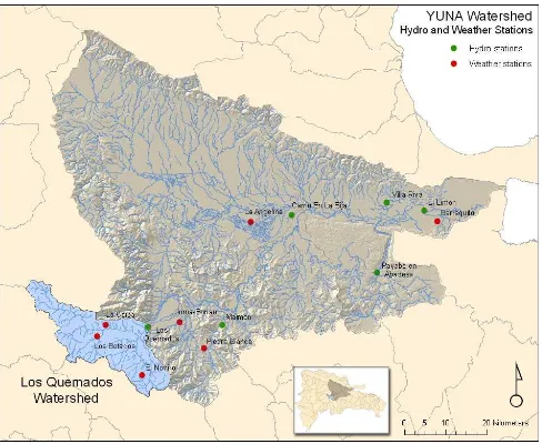
Located in the central and northeastern portion of the Dominican Republic, the Yuna flows 138.6 km from the east part of Cerro Montoso and in the south of Firme Colorado at 1150 meters of elevation, as it flows through the Cibao eastern plain to the ecological significant Samana Bay. Replenished by several significant tributaries (Arroyo Blanco, Masipedro, Maimon, Camu, Barracote, etc.) and controlled by several dams (Blanco, Arroyan, Tiretio, Yuboa, Hatillo, Rincon, Guaygui), the Yuna is the largest of watershed in Hispaniola and has a total area of 5498 square kilometers.
Temperatures
Weather in the watershed is variable. At the head of the Rio Blanco temperatures are low due to its proximity to the Alto Bandera mountains (2500 msnm). In its upper reaches, at the Los Botados and El Novillo climatologic stations, temperature range between 12-23°C. In contrast, temperatures along the Payabo River and lagoons are are higher as they are within the foothill system of Los Haitíses which do not exceed 550 msnm. Temperatures throughout the entire Yuna watershed range from between 12-31°C.
1
Figure 1. General Reference Map of the Yuna Watershed in the Dominican Republic showing distribution of hydrologic and weather stations and the Los Quemados sub-watershed.
Rainfall
The Yuna watershed is one of the most humid parts of the country and the Yuna River carries the largest water volume in Eastern Hispaniola. Areas of high rainfall may exceed 3000 mm/year, while in the tributaries on the southern side of the Septentrional mountain chain, temperatures are higher and there is less rainfall, with resultant less channel flow.
Vegetation
Yuna watershed has a good vegetation cover, especially in the sub-watersheds of Maimón, Arroyo Blanco, Masipedro, Jima and Camú. In this area, plantations of Pinus, long leave tress, manaclares, and coffee and cacao crops can be observed, but in the case of Blanco River the situation is different, due to influence of Tireo River which watershed is completely eroded and with intense agriculture activities.
In the lower Yuna valley, the main activity is agriculture, particularly rice farming which occupies 95% of the area suitable for farming. For rice farming a large quantity of water is utilized from Yuna River and its tributaries, plus the inflows that come from Los Haitises area though lagoons and springs. The portion that forms part of the estuary has the largest mangrove reserve of the Hispaniola occupying an area of 70.22 km2 disseminated across the Yuna mouth and to the whole wide of the Bay, extending more than five kilometers through the wetlands located in the proximities of Ciénaga de Barracote, Laguna Cristal, Guayabo and Los Haitises.
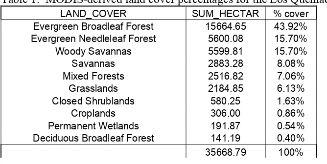
There exists two current datasets of land cover for the Yuna watershed. This includes a) the 30m Landsat ETM+ derived land cover that was provided by the Dominican Republic Ministry of the Environment and comprise nearly 40 land cover classes from year 2000; and b) the 1000m MODIS-derived land cover that is part of the Global Land Cover Classification initiative and comprises 17 classes from the year 2000. Table 1 shows the representation of land cover percentages for the Los Quemados watershed, the predominant vegetation type is Evergreen Broadleaf forest (43.9%) followed by 15.7% Evergreen needle leaf Forest and 15.7% Woody Savannas. The remaining vegetation landcover includes savannas, mixed forests and grasslands.
Table 1. MODIS-derived land cover percentages for the Los Quemados watershed.
LAND_COVER SUM_HECTAR % cover
Evergreen Broadleaf Forest 15664.65 43.92% Evergreen Needleleaf Forest 5600.08 15.70% Woody Savannas 5599.81 15.70%
Savannas 2883.28 8.08%
Mixed Forests 2516.82 7.06%
Grasslands 2184.85 6.13%
Closed Shrublands 580.25 1.63%
Croplands 306.00 0.86%
Permanent Wetlands 191.87 0.54% Deciduous Broadleaf Forest 141.19 0.40%
35668.79 100%
Hydrostation Summary
Table 2. Hydrostation Summary: Average Annual Discharge in m3/sec.
Station Name Ann.Mean (m3/sec) Min Max Period
Los Quemados 15.83 2.42 (4/65) 56.52 (9/76) 1962-79
Maimón 5.15 0.12 (9/91) 40.03 (9/98) 1968-00
La Bija 36.23 2.79 (7/75) 145.88 (11/96) 1968-02
Villa Riva 89.38 6.08 (3/77) 402.52 (5/79) 1956-92
Payabo 5.79 0.47 (3/77) 22.68 (5/83) 1971-95
El Limón 102.39 10.87 (4/75) 374.68 (5/81) 1968-03
II. Water Balance of the Yuna & Los Quemados Watersheds (Excel model)
A Water Balance was calculated for the entire Yuna Watershed above El Limon Hydrostation (located at 8 m elevation) and as well for a subwatershed in the Northwestern portion of the watershed above the Los Quemados Hydrostation (located at 1225 m elevation). The two watersheds we will name Yuna, which comprises an area of over 5498 km2 and the Quemados, which is over 363 km2.
Precipitation (P)
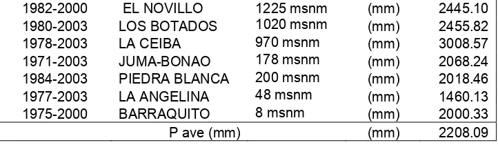
Monthly precipitation data was available from seven different climatic stations within the Yuma watershed. Average annual precipitation ranged from 146.0 cm (La Angelina) to 300.8 cm (La Ceiba) for the time periods available. Average annual precipitation for all seven sites was 220.8 cm per year.
For the Yuna waterbalance, the average monthly precipitation amounts from all seven available hydrostations were averaged over the published time periods of record. The lowest monthly average was calculated for February at 121.11 mm and the highest monthly average was calculated for May at 272.15 mm. The annual average for all stations was 2208 mm.
Table 5. Precipitation, elevation & time series from seven weather stations in the Yuna watershed.
1982-2000 EL NOVILLO 1225 msnm (mm) 2445.10 1980-2003 LOS BOTADOS 1020 msnm (mm) 2455.82
1978-2003 LA CEIBA 970 msnm (mm) 3008.57
1971-2003 JUMA-BONAO 178 msnm (mm) 2068.24 1984-2003 PIEDRA BLANCA 200 msnm (mm) 2018.46 1977-2003 LA ANGELINA 48 msnm (mm) 1460.13
1975-2000 BARRAQUITO 8 msnm (mm) 2000.33
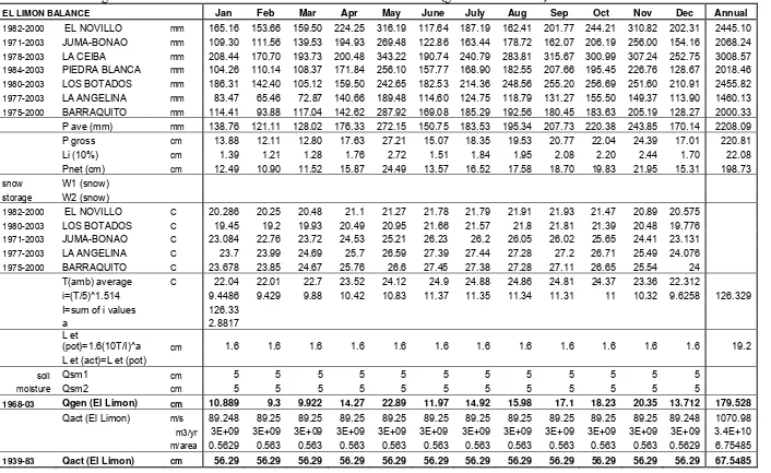
Table 3. Water budget calculations for the Yuna Watershed at El Limon Watershed (generated & actual)
EL LIMON BALANCE Jan Feb Mar Apr May June July Aug Sep Oct Nov Dec Annual
1982-2000 EL NOVILLO mm 165.16 153.66 159.50 224.25 316.19 117.64 187.19 162.41 201.77 244.21 310.82 202.31 2445.10
1971-2003 JUMA-BONAO mm 109.30 111.56 139.53 194.93 269.48 122.86 163.44 178.72 162.07 206.19 256.00 154.16 2068.24
1978-2003 LA CEIBA mm 208.44 170.70 193.73 200.48 343.22 190.74 240.79 283.81 315.67 300.99 307.24 252.75 3008.57
1984-2003 PIEDRA BLANCA mm 104.26 110.14 108.37 171.84 256.10 157.77 168.90 182.55 207.66 195.45 226.76 128.67 2018.46
1980-2003 LOS BOTADOS mm 186.31 142.40 105.12 159.50 242.65 182.53 214.36 248.56 255.20 256.69 251.60 210.91 2455.82
1977-2003 LA ANGELINA mm 83.47 65.46 72.87 140.66 189.48 114.60 124.75 118.79 131.27 155.50 149.37 113.90 1460.13
1975-2000 BARRAQUITO mm 114.41 93.88 117.04 142.62 287.92 169.08 185.29 192.56 180.45 183.63 205.19 128.27 2000.33
P ave (mm) mm 138.76 121.11 128.02 176.33 272.15 150.75 183.53 195.34 207.73 220.38 243.85 170.14 2208.09
P gross cm 13.88 12.11 12.80 17.63 27.21 15.07 18.35 19.53 20.77 22.04 24.39 17.01 220.81
Li (10%) cm 1.39 1.21 1.28 1.76 2.72 1.51 1.84 1.95 2.08 2.20 2.44 1.70 22.08
Pnet (cm) cm 12.49 10.90 11.52 15.87 24.49 13.57 16.52 17.58 18.70 19.83 21.95 15.31 198.73
snow W1 (snow)
storage W2 (snow)
1982-2000 EL NOVILLO C 20.286 20.25 20.48 21.1 21.27 21.78 21.79 21.91 21.93 21.47 20.89 20.575
1980-2003 LOS BOTADOS C 19.45 19.2 19.93 20.49 20.95 21.66 21.57 21.8 21.81 21.39 20.48 19.776
1971-2003 JUMA-BONAO C 23.084 22.76 23.72 24.53 25.21 26.23 26.2 26.05 26.02 25.65 24.41 23.131
1977-2003 LA ANGELINA C 23.7 23.99 24.69 25.7 26.59 27.39 27.44 27.28 27.2 26.71 25.49 24.076
1975-2000 BARRAQUITO C 23.678 23.85 24.67 25.76 26.6 27.45 27.38 27.28 27.11 26.65 25.54 24
T(amb) average C 22.04 22.01 22.7 23.52 24.12 24.9 24.88 24.86 24.81 24.37 23.36 22.312
i=(T/5)^1.514 9.4486 9.429 9.88 10.42 10.83 11.37 11.35 11.34 11.31 11 10.32 9.6258 126.329
I=sum of i values 126.33
a 2.8817
L et
(pot)=1.6(10T/I)^a cm 1.6 1.6 1.6 1.6 1.6 1.6 1.6 1.6 1.6 1.6 1.6 1.6 19.2
L et (act)=L et (pot)
soil Qsm1 cm 5 5 5 5 5 5 5 5 5 5 5 5
moisture Qsm2 cm 5 5 5 5 5 5 5 5 5 5 5 5
1968-03 Qgen (El Limon) cm 10.889 9.3 9.922 14.27 22.89 11.97 14.92 15.98 17.1 18.23 20.35 13.712 179.528
Qact (El Limon) m/s 89.248 89.25 89.25 89.25 89.25 89.25 89.25 89.25 89.25 89.25 89.25 89.248 1070.98
m3/yr 3E+09 3E+09 3E+09 3E+09 3E+09 3E+09 3E+09 3E+09 3E+09 3E+09 3E+09 3E+09 3.4E+10
m/area 0.5629 0.563 0.563 0.563 0.563 0.563 0.563 0.563 0.563 0.563 0.563 0.5629 6.75485
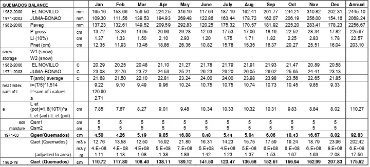
Table 4. Water budget calculations for Los Quemados Watershed
QUEMADOS BALANCE Jan Feb Mar Apr May June July Aug Sep Oct Nov Dec Annual
1982-2000 EL NOVILLO mm 165.16 153.66 159.50 224.25 316.19 117.64 187.19 162.41 201.77 244.21 310.82 202.31 2445.10
1971-2003 JUMA-BONAO mm 109.30 111.56 139.53 194.93 269.48 122.86 163.44 178.72 162.07 206.19 256.00 154.16 2068.24
1982-2000 Paveg mm 137.23 132.61 149.52 209.59 292.83 120.25 175.32 170.57 181.92 225.20 283.41 178.23 2256.67
P gross cm 13.72 13.26 14.95 20.96 29.28 12.03 17.53 17.06 18.19 22.52 28.34 17.82 225.67
Li (10%) cm 1.37 1.33 1.50 2.10 2.93 1.20 1.75 1.71 1.82 2.25 2.83 1.78 22.57
Pnet (cm) cm 12.35 11.93 13.46 18.86 26.36 10.82 15.78 15.35 16.37 20.27 25.51 16.04 203.10
snow W1 (snow)
storage W2 (snow)
1982-2000 EL NOVILLO C 20.29 20.25 20.48 21.10 21.27 21.78 21.79 21.91 21.93 21.47 20.89 20.58
1971-2003 JUMA-BONAO C 23.08 22.76 23.72 24.53 25.21 26.23 26.20 26.05 26.02 25.65 24.41 23.13
T(amb) average C 21.68 21.50 22.10 22.81 23.24 24.00 24.00 23.98 23.98 23.56 22.65 21.85
heat index i=(T/5)^1.514 9.22 9.10 9.49 9.96 10.24 10.75 10.75 10.74 10.73 10.45 9.85 9.33
sum of i I=sum of i values 120.60
a 2.71
e
L et
(pot)=1.6(10T/I)^a cm 7.85 7.67 8.27 9.01 9.48 10.34 10.33 10.32 10.31 9.83 8.84 8.02 110.27
L et (act)=L et (pot)
soil Qsm1 cm 5 5 5 5 5 5 5 5 5 5 5 5
moisture Qsm2 cm 5 5 5 5 5 5 5 5 5 5 5 5
1971-03 Qgen(Quemados) cm 4.50 4.26 5.19 9.85 16.88 0.48 5.44 5.04 6.06 10.43 16.67 8.02 92.83
Qact (Quemados) m3/s 12.76 13.58 12.50 15.92 21.80 16.31 14.23 15.75 17.59 19.24 18.79 23.96 202.42
m3/y 4.E+08 4.E+08 4.E+08 5.E+08 7.E+08 5.E+08 4.E+08 5.E+08 6.E+08 6.E+08 6.E+08 8.E+08 6.E+09
(adjusted to area) m 1.11 1.18 1.08 1.38 1.89 1.42 1.23 1.37 1.53 1.67 1.63 2.08 17.56
For the Quemados waterbalance, the average monthly precipitation amounts were taken from two nearby hydrostations (El Novillo and Juma Bonao). The lowest monthly average was calculated for June at 120.25 mm and the highest monthly average was calculated for May at 292.83 mm and 283.41 mm in November. The annual average for both stations nearly 2257 mm.
Table 6. Precipitation, elevation and time series data from 2 weather stations in the Los Quemados watershed.
1982-2000 EL NOVILLO 1225 msnm 2445.10 (mm) 1971-2003 JUMA-BONAO 178 msnm 2068.24 (mm)
Pave (mm) 2256.67 (mm)
Interception Loss (Li)
Estimated at 10%. The actual amount may be lower in the upper watershed and higher in the lower watershed due to vegetated terrain. Though the actual vegetation cover may affect the interception losses from the net precipitation, the overall variation was estimated here as 10% on average.
Net Precipitation (Pn)
Net precipitation was obtained by subtracting Li from P (P-L = Pn)
Snow data (W)
Subtropical climate and no snow even at the highest elevation within watershed – lowest recorded temperatures around 10 degrees Celsius. Therefore No snow or glacial inputs within watershed, calculated as zero.
Evapotranspiration Loss – potential and actual (Let (pot) a& Let (act))
Palmer and Havens2 provides the methodology for calculating monthly potential
evapotranspiration using Thornthwaite’s empirical formulas. The Thornthwaite method3 uses air temperature as an index of the energy available for evapotranspiration and assumes that air temperature is correlated with the integrated effects of net radiation and other controls of evapotranspiration. Using this method, there is no correction for different vegetation types. The empirical formula developed by Thornthwaite is
Let(pot) = 1.6 (10T/I)^a where Let = potential evapotranspiration in cm/mo, T = mean monthly air temperature in C, I = annual heat index or the sum of the index values, i, where i = (T/5)^1.514.
Using an average of the available monthly temperature records for five sites for the Yuna watershed and two sites for Los Quemados, the average 1982-2000 year heat index (I) was calculated as 126.3 for the Yuna and 120.6 for Los Quemados, a was also determined4 and subsequent monthly potential evapotranspiration, Let(pot).
2
Palmer, WC and AV Havens (1958) “A Graphical Technique for Determining Evapotranspiration by the Thornthwaite Method, Monthly Weather Review, March 6, 1958.
3
Dunne T and LB Leopold (1978), Water in Environmental Planning, Freeman & Company, p. 136-37.
4
For the Yuna watershed, potential evapotranspiration was nearly 19.2 cm/year (considerably less than the reported ET (pot) at El Limon between 134.5 and 144.6 cm/year). For Los Quemados, potential evapotranspiration was nearly 94.5 cm/year (comparable to reported ET (pot) at El Novillo at 98.7 cm/year).
We can also use vegetation type to estimate ET. Within the Quemados watershed using 44% Evergreen Broadleaf forest, 16% Evergreen needle leaf Forest and 16% Woody Savannas. The remaining vegetation landcover includes savannas, mixed forests and grasslands. ET estimates for North American forested types range from ____ in one particular summary paper.
Soil Moisture (Qsm)
When moisture conditions are suitable, the actual rate of evapotranspiration is equal to the potential rate. Government data regarding soils in the Quemados watershed show three types of which one type5 is predominant throughout the watershed. We know little about these soil classifications but could assume soil moisture holding capacity of approximately 60-70% forested slopes, 15% woody savannas, and the remainder (~15%) of grasslands and savannah. Ideally we would be able to have field data approximating the soil moisture conditions at the beginning and end of the month and use these values to adjust discharge generation for our model. As a rough estimate, 5 cm was designated average field
capacity. Short of any real data we have assumed continual adequate moisture abundance in the soil and therefore a net difference in soil moisture (Qsm) of zero. In actuality there may be significant temporal variation of moisture contribution from this term.
Discharge generated and actual (Qgen & Qact)
Generated flow (Qgen) was attined by subtracting Let(act) and the difference in soil moisture content at the beginning and end of the month from net precipitation Qgen = Pnet – Let – (Qsm2 – Qsm1) – (W2-W1)
Using the above approximations and simplifications, the effective inputs for Qgen are simply Pnet and Let. Let is temperature dependent and is highly dependent on the value of the heat index, I. Temperature values were averaged from ambient readings and therefore can cause error in the calculation of i, I and a. This model is able to take sparse data and estimate water production at a specific point. Qact data (in m3/sec) were correlated to cm/yr for the approximate Yuna watershed area of 5000 km2 above El Limon and likewise for the 363 km2 watershed area above Los Quedamos hydrostation.
For the Yuna, the total annual flow generated was 179.5 cm/yr which was higher than the reported average annual discharge of 67.55 cm/year for the 1939-83 period at El Limon.
For Los Quemados, the total annual flow generated was 124.6 cm/yr which was lower than the reported 929.2 cm/year for the 1962-79 period at Los Quemados station.
5
Discussion of Results:
Flow generation calculations for Yuna watershed are higher than actual. Flow generation calculations for Los Quemados watershed are lower than actual. However, given the assumptions and the data gaps for this type of calculation, the results are within the same order of magnitude and can be considered quite satisfactory.
Quite possibly an adjustment in the Li and ET values for this model may well influence the generated flow in exactly the opposite manner and to bring the estimated and actual
numbers closer together. For instance, the lower Yuna would have less interception loss but higher rates of evapotranspiration due to higher temperatures and exposure; while Los Quemados would have more interception loss and lower rates of evapotranspiration from higher elevations, steeper slopes and greater forested canopy.
There are a number of additional adjustments causes of error that may influence the overall water budget calculations. Consider these:
Precipitation and temperature data were taken from different and non-overlapping years. For instance, the seven stations used to generate rain data for the Yuna covered different time periods between 1971 and 2003, while the flow data was reported at El Limon for the period of 1939-83. Likewise, the two stations (El Novillo and Juma Bonao) used to generate rain data for Los Quemados covered time periods between 1971 and 2003, while the flow data was reported at Los Quemados station was from the period of 1962-79. As well, El Novillo station is located at 1225 m msnm and Juma Bonao is located at 178 msnm though it is located only ___ m away as a crow flies. Rainshadow and temperature effects may also influence these sites.
In addition, we have only monthly average temperatures, rather than daily, maximum or minimum temperatures. We have no soil moisture storage information and here assume that this influence is negligible. Inaccuracies of temperature and precipitation collection also exist on steep terrain as is found in Quemados; the relatively flat areas in the lower Yuna create inaccuracies of flow. Finally, the Yuna watershed has more than half a dozen major dams, levies, dikes and channels. The lower Yuna is heavily used for agriculture, especially rice, for which water is diked, diverted, ponded and then drained at different times of the year. The influence of return flows is also likely more significant at El Limon that at other upstream and less managed sites.
III. Obtaining readily available satellite data for the Water Budget model:
Tropical Rainfall Measuring Mission (TRMM)
TRMM6 is a joint mission between the National Aeronautics and Space Administration (NASA) of the United States and the Japan Aerospace Exploration Agency (JAXA). The
6
Kummerow, C., Barnes, W., T. Kozu, J. Shiue, and J. Simpson, 1998: The tropical rainfall measuring mission (TRMM) sensor package, J. Atmos. Oceanic Technol., 15, 809-817.
satellite was launched in November of 1997 and is currently continuing to operate. It is in a low inclination orbit covering the tropics between approximately 40S to 40N latitude. The primary rainfall sensors on board the TRMM spacecraft include the 13.8 GHz Precipitation Radar (PR) and the TRMM Microwave Imager (TMI). In addition, TRMM carries the Visible and Infrared Radiometer (VIRS), the Clouds and Earth's Radiant Energy System (CERES), and the Lightning Imaging System (LIS), which provide detailed information of rainfall over the tropics.
The TRMM PR is the first and currently the only precipitation radar in space. It provides detailed information on the three-dimensional structure of rain systems with a horizontal resolution of approximately 4-km and a total of 80 levels in the vertical with a resolution of 250 meters. The PR is a cross-track scanner with a relatively narrow swath width (~215 km), however, which results in limited sampling for climate. Although the sampling of the PR is much more limited than most satellite rain sensors, the PR provides a far more detailed look at tropical rain systems than is available from any other current or previous spaceborne rainfall sensor. More details regarding the TRMM instrument specifications are given by Kummerow et al. [1998, 2000].
The data for this exercise was downloaded at the TRMM Online Visualization and Analysis System (TOVAS) found at http://lake.nascom.nasa.gov/tovas/3B43/
This interface is designed for visualization and analysis of the TRMM and other Satellite monthly rainfall product, 3B43 (Version 6.0). Users can generate plots or ASCII Output for area average (Area Plot), time series (Time Plot), and Hovmoller diagram. Additional description of the file format for this product is available at:
http://tsdis02.nascom.nasa.gov/tsdis/Documents/ICSVol4.pdf
ASCII output files were used to generate point shapefiles in ArcView GIS 3.3, reprojected from Geographic coordinates to UTM WGS84 Zone 19.The original data contains monthly rainfall at a point spatial resolution of 0.25В° x 0.25В°. The reprojected points where then interpolated to create a 4 x 4 km GRID surface using universal kriging. Once a GRID surface was created, the precipitation values were summed by watershed for year 2000.
Moderate Resolution Imaging Spectroradiometer (MODIS) Land Cover
This exercise used the MODIS7 Land Cover Classification product, MOD12Q1, which identifies 17 classes of land cover in the International Geosphere-Biosphere Programme (IGBP) global vegetation classification scheme. This scheme includes 11 natural vegetation classes, 3 developed land classes, one of which is a mosaic with natural vegetation,
permanent snow or ice, barren or sparsely vegetated, and water. These classes are distinguished with a supervised decision tree classification method. The MOD12 classification schemes are multitemporal classes describing land cover properties as observed during the year (12 months of input data). Successive production of this "annual" product allows us to make new land cover maps with increasing accuracies as both
classification techniques and the training site database mature. The data was downloaded in HDF format from the Land Processes Distributed Active Archive Center (LP DAAC) at
http://edcdaac.usgs.gov/ More information about this product can be obtained from
http://edcdaac.usgs.gov/modis/mod12q1.asp or from Belward et al, (1999) and Hansen et al, (2000).
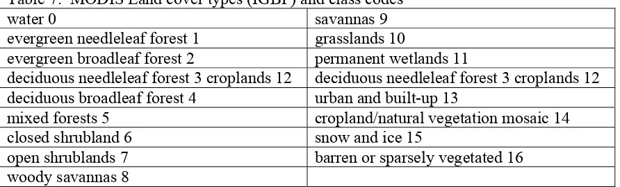
Table 7. MODIS Land cover types (IGBP) and class codes
water 0 savannas 9
evergreen needleleaf forest 1 grasslands 10
evergreen broadleaf forest 2 permanent wetlands 11
deciduous needleleaf forest 3 croplands 12 deciduous needleleaf forest 3 croplands 12 deciduous broadleaf forest 4 urban and built-up 13
mixed forests 5 cropland/natural vegetation mosaic 14 closed shrubland 6 snow and ice 15
open shrublands 7 barren or sparsely vegetated 16 woody savannas 8
Moderate Resolution Imaging Spectroradiometer (MODIS) Land Surface Temperature
MODIS temperature products are key inputs to many of the high level MODIS products and provide data for global temperature mapping and change observation. On land, soil and canopy temperature are among the main determinants of the rate of growth of vegetation and they govern seasonal start and termination of growth. Hydrologic processes such as evapotranspiration and snow and ice melt are highly sensitive to surface temperature fluctuation, which is also an important discriminating factor in classification of land surface types. The MODIS Land Surface Temperature (LST) products provide per-pixel temperature values. Averaged temperatures are extracted in Kelvin with a day/night LST algorithm applied to a pair of MODIS daytime and nighttime observations. This method yields 1 K accuracy for materials with known emissivities, and view angle information is included in each LST product. The LST algorithms use MODIS data as input, including geoposition, radiance, cloud masking, atmospheric temperature, water vapor, snow, and land cover.
7
Belward, A. S., J. E. Estes, and K. D. Kline, The IGBP-DIS Global 1-km Land-Cover Data Set DISCover: A Project Overview, Photogram. Eng. Remote Sens., 65, 1013-1020, 1999.
There are seven LST data products which are archived in Hierarchical Data Format - Earth Observing System (HDF-EOS) format files and can be downloaded from the Land
Processes Distributed Active Archive Center (LP DAAC) at http://edcdaac.usgs.gov/ The LST products have a nominal pixel spatial resolution of 1km at nadir and a nominal swath coverage of 2030 or 2040 lines by 1354 pixels per line. These data product are
georeferenced to latitude and longitude centers of 1 km resolution pixels and in a gridded map projection format referred to as tiles. Each tile is a piece, e.g., about 1113km by 1113km in 1200 rows by 1200 columns, of a map projection. This exercise used the MOD11C3 product, which was released on June 2003, and provides monthly composited and averaged temperature values at 0.05 degree latitude/longitude grids, as well as the averaged observation times and viewing zenith angles for daytime and nighttime LSTs. More information on LST products can be found at
http://www.icess.ucsb.edu/modis/modis-lst.html and
http://edcdaac.usgs.gov/modis/mod11c3v4.asp
Moderate Resolution Imaging Spectroradiometer (MODIS) Evapotranspiration (ET)
At the time of writing this report, the MODIS science team was working on the release of a beta version of the MODIS-derived evapotranspiration (ET) product (MOD16). This product, once properly calibrated, will have a temporal resolution of eight days at a spatial resolution of 1 km (over the land surface only) and will be a tremendous benefit for improving water budget models. These data will be combined with a land Surface Resistance product that captures sub-optimum conditions produced by soil/atmospheric moisture deficits for vegetation photosynthesis and transpiration. Both evapotranspiration and surface resistance are two parameters essential to global modeling of climate, water balance, and trace gases. In addition, they are required in estimating photosynthesis, respiration, and net primary production. The Surface Resistance product will be calculated using the MODIS Land Surface Temperature (MOD11) and the MODIS modified
IV. Adaptation of Data to SWBM Model
We started this project looking for a simple model with spatial capabilities to map and predict water budgets. First we reviewed the literature and the two possibilities were a complicated and data intensive Soil and Water Assessment Tool (SWAT), and a less data intensive Spatial Water Budget Model (SWBM) which was field tested for small
watersheds in Latin America. SWBM was investigated and determined to be the best choice and the base maps and data was prepared/collected/requested for this purpose. SWBM is an ArcView GIS 3.x Avenue extension and was developed as part of a methodology for assessing water availability and use under different development pathways at a watershed scale.
As described by Luijten et al. (2000)8, the Spatial Water Budget Model (SWBM) is a continuous, distributed parameter, watershed scale model that simulates water supply and demand over space and time on a daily basis using GIS data structures. SWBM delineates streams and computes availability of stream water as it flows downstream or is (partly) extracted for domestic, industrial and agricultural uses. It is a tool for assessing water availability and use under different development pathways at a watershed scale to determine whether water security is a potential problem, and if so, when and where it occurs. It was intended for supporting local decision-making processes and for teaching local stakeholders about basic landscape responses. The model was designed specifically for the needs and resources of developing countries in Latin America and the Caribbean, but can be applied watersheds in other areas as well. The model was not designed for engineering specific hydrologic projects or for describing the movement of water based on detailed physical processes. Processes that are simulated by SWBM are: (i) land unit water balance, (ii) water flow to streams, (iii) stream water flow balance, (iv) water storage in dams and small reservoirs, and (v) water extraction from reservoirs and streams for domestic, agricultural and industrial uses. The model does not simulate peak flow, sediment loading, soil erosion and vegetation growth. However, the effects of different crop development stages on evapotranspiration are accounted for by monthly lookup tables.
Upon data compilation and preparation for running the model for the Yuna watershed, we encountered many problems. Upon using the SRTM 90m digital elevation model (DEM) we were advised by the creator of the program (Joep Lutjen) that our data was of very poor quality and hydrologically inconsistent. Upon filling the NoData values in the DEM,
approximately 18% of the grid cells had a zero slope percentage, which caused the program to crash. For proper operation of the SWBM model, there should be little to none of grid cells that have zero slope. One important recommendation is to try and avoid the SRTM 90m product, especially in flat (non-slope) areas. In addition, one should obtain DEM values to floating point format (not integer). This will make a large difference when working in flatter areas because any difference in elevation between adjacent grid cells, no matter how small, will allow the proper calculation of flow direction. Burning in rivers could help delineate a consistent stream network but it will not solve the problem of the
8
many zero-slope grid cells which produce errors in the flow routing. If SRTM 90m data is the only elevation available one should download the data from the CIAT SRTM website, where they have developed an algorithm to fill the NoData holes and has made an entire duplicate of the SRTM data archive available with holes filled.
http://gisweb.ciat.cgiar.org/sig/90m_data_tropics.htm
Another problem we encountered was the size of our watershed. In the SWBM user
manual, it suggested that SWBM was specifically developed for watershed up to 50,000 ha. SWBM does not have any grid size limitation, but the programmer advises against using very large grids because the simulation runs will be annoyingly slow. For every simulated day, approximately 45 grid evaluations are being carried out. Ideally, each evaluation is completed in <1 second, otherwise a simulation run will be very slow. (SWBM functions slow down considerably and consume more memory as the simulation progresses due to ArcView's poor memory management). The model can be applied to large watersheds but one has to be aware of the technical pitfalls and simulation times will be quite long. The main problem with simulating larger watershed is that SWBM will not simulate delays in water flow in the streams. In other words, water that ends up in a stream anywhere in the watershed is assumed to reach the watershed outlet that same day. Consequently, day-to-day variations in simulated stream flow rates at the watershed outlet will be much larger than in reality resulting in unrealistically high simulated peak flow on rainy days. When splitting up large watershed and simulating each subbasin separately, SWBM is still not able to account for a delay in river flow.
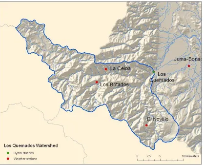
Because of these difficulties, we decided to select a subwatershed with adequate slope and fewer hydrologic interferences such as dams and levees. This subwatershed would require a hydrostation for calibration purposes. The Los Quemados watershed was chosen because it was in itself a hydrostation and was located in the upper reaches of the Yuna, where there was adequate slope variation, encompassing just over 363 km2 and comprising terrain from 1500 to 1225 msnm elevation. The two comparable weather stations that were used were El Novillo and Juma-Bonao. In addition, we downloaded satellite data from TRMM and MODIS to generate daily and monthly precipitation and temperature data. Although we continued to have problems running the model and did not obtain the desired model results, we feel that additional time and resources spent on model experimentation would be
worthwhile for future investigations. For this reason, we present a quick tutorial of the SWBM model and a brief discussion on the issues we encountered.
Data requirements
Different from excel model presented previously (which requires little more than monthly averages of temperature, precipitation), SWBM requires data to be presented in look-up tables with Julian day values of maximum and minimum temperatures, precipitation and solar radiation. Other look-up tables correlate stored parameters for land cover, infiltration, wilting point, soil moisture, and ET for the watershed of interest.
SWBM model output
The model runs create an output file that can be used in analyzing water availability and to create hydrographs of the rive systems at various points. There is also a routine that allows one to introduce human influences such as withdrawals for urban and agricultural uses, storage in reservoirs and hydropower stations – however, we did not have access to this sort of information in order to generate this additional level of analysis.
In the Appendices to this document, we have created a start-up guide for users of SWBM followed by details of the program functions and capabilities. Additional information can be found in the SWBM manual, a copy of which is available at
A
PPENDIX1
SWBM procedures
Create File Directory Structure
1- Create file data structure within SWBM folder/regions directory (e.g. Yuna region should have 4 folders: grids, tables, results, weather)
2- GRIDS directory should also have 4 folders: info, slope, dem, landcover 3- Use ArcView Data Manager to move grids to the appropriate folder
4- Using the ArcView data manager, copy the grids (dem, slope, landcover) to the appropriate grids folder, move or delete grids that are not needed
5- Default: OS Env variables (specifies location of regions directory) SWBM=C:\SWBM
HOME=C:\TEMP 6- Set working directory
NOTES
- use floating point format (i.e., 1.032, 3.08957) for all grids (DEM, slope, strnet,…) except Landcover which should be in integer (i.e., 1, 50) format since it references a landcover lookup table
- each grid must have the same cell size, minimum / maximum starting coordinates, and projection defined
- for example, in the YUNA watershed we use a projection of: UTM zone 19 units meters datum WGS84
- grid names cannot exceed 10 characters
Getting Started
1- Start Up ArcView 3.3
2- At prompt: select open new view
3- At prompt: do you want to add data to view Æ select No
4- Under File: Extensions – check SWBM model 1.3 (SWBM Hydrological tools box not necessary or Hydro Tools will appear on menu twice); also ensure that Spatial Analyst extensions are also enabled
5- Under Hydro Tools,
a. Add Existing Grid Æ select appropriate Elevation Grid b. At prompt: select map units Æ Meters
c. Identify sinks in the DEM d. Fill sinks in the DEM e. Calculate Slope
f. Compute Flow Direction
g. --- stop there -- // go to SWBM main
6- Under SWBM Main,
b. Select appropriate map units for view Æ meters, Okay c. Select input grids for watershed
i. DEM
ii. DEM stream network iii. Land use classes iv. DEM based slope
v. Under Hydraulic conductivity, Select Æ Cancel, then type in units of 1, click Okay
SWBM procedures
1- Open ArcView; add view for new watershed; call up DEM 2- Under HYDRO_tools: add existing grid (find DEM for region) 3- Highlight DEM view; Under HYDRO_tools: identify existing sinks 4- Under HYDRO_tools: fill existing sinks
5- Open ArcView project (apr file) – e.g. Cabuyal
a. Under File: select open project, go to SWBM folder, double click .apr project (SWBMmain_13.apr)
b. Set working directory for project
6- If project is incomplete, go to Hydro Tools and add existing grid 7- If project is complete, go to SWBM main and select region
a. Double click to correct folder (SWBM\regions\...) b. Single click watershed (CABUYAL_100)
c. From prompt: Specify map units (meters)
d. From prompt: Specify input grids (self populated from grids folder within watershed folder: SWBM\regions|cabutal\grids\dem, strnet, landuse, slope, hydraulic conductivity)
8- Under SWBM main: select Land Use parameters to edit fields; includes: a. Descriptive land use names
h. NOTE: these parameters are stored in dbf format in the look up tables in the watershed folder (SWBM\regions\cabuyal\tables\landuse.dbf etc.)
9- Under SWBM Main: select Hydrologic soil parameters to edit fields; includes: a. Generic ET coefficient
k. Maximum flowlength, FLOWLMX (m)
10-Under SWBM Main: select Output points located in tables folder, file labeled output_points.dbf (e.g. SWBM\regions\cabuyal\tables):
11-Under SWBM Main: select Weather Station Options to edit fields 12-Under SWBM Main: select to Water Use specifications to edit fields
To RUN MODEL
APPENDIX II: Background and essential information on SWBM
J.C.Luijten, J.W. Jones and E.B. Knapp (200): Spatial Water Budget Model and GIS Hydrological Tools (an ArcView GIS extension, updated for model v. 1.3), developed by the Universty of Florida9 of ICASA10 90 pp.
The Spatial Water Budget Model (SWBM) was developed as part of dissertation research of the first author at the Crop Modeling Systems Laboratory at the University of Florida as part of a larger research program at CIAT in Colombia. SWBM has been successfully applied to the Cabuyal River watershed in southwest Colombia and the Tascalapa watershed in central Honduras. The full scientific documentation of SWBM is: Luitjen, J.X., 1999. a tool for community-based water resources management in hillside
watersheds. Ph.D. dissertation. University of Florida. Gainesville, FL. 303 pp.
http://etc.fcla.edu/etd/uf/1999/amp7392/luijten.pdf. Two other publications that discuss the technical aspects of SWBM and its application include: Luitjen, J.C., J.W. Jones, and Knapp, 2000. Dynamic modeling of strategic water availability in the cabuyal River, Colombi: The impact of land cover change on the hydrological balance. Advances in Environmental Monitoring and Modelling 1(1): 36-60.
http://www/kcl.ac.uk/kis/schools/hums/geog/advemm/vol1no1.html.
SWBM now has the capability to use weather data from multiple weather stations and it can spatially interpolate those data on a daily basis.
SWBM is a continuous, distributed parameter, watershed scale model that simulates water supply and demand over space and time on a daily basis using GIS data structures. SWBM delineates streams and computes availability of stream water as it flows down slope or is extracted for domestic, industrial and agricultural uses. The model simulates the effects on hydrology and water yields of changes in land use, water use for domestic, industrial and agricultural purposes, locations of water extraction and impedance by dams on a daily basis.
Processes that are simulated by SWBM are: i) land unit water balance, ii: water flow to streams, iii: stream water flow balance, iv) water storage in dams and small reservoirs, and v) water extraction from reservoirs and streams for human uses. The model does not simulate peak flow, sediment loading, soil erosion, and vegetation growth.
SWBM is a tool for assessing water availability and use under different development pathways at a watershed scale to determine whether water security is a potential problem, and if so, when and where it occurs. The model has been developed for agricultural hillside watersheds in Latin America and the Caribbean for basins up to approx, 50,000 ha in size and for which few biophysical data area available. Simulation results obtained with SWBM can be used for supporting local decision-making processes to guide development ot the benefit of local communities, as well as for teaching local stakeholders about basic functions of multiple community watershed components.
9
Agricultural and Biological Engineering, University of Florida, Gainesville, FL
10
SWBM has been programmed in Avenue (ESRI, 1996) the scripting language of ArcView GIS software and run on Windows and Unix based systems on which ArcView GIS 3.1 or higher and Spatial Analyst v1.1 extension have been installed. Data are inputted through ARC/INFO grids and through user-friendly menus. Simulation results, which are saved in ARC/INFO grids and in dBase-IV files, can be processed using Avenue scripts and
spreadsheet software.
p.9 – minimum hardware:
MS windows PC w/Pentium 200 MHz processor and 200 MB hard disk space recommended hardware:
MS windows PC w/Pentium II/III 500 MHz processor, fast SCSI disk and 1 GB hard disk space
1.2 (p.10) installation, self extracting zip file (swbm_v13.exe), direct to root of file system (C or D). New directory named SWBM will be created with model and data)
Opt. 1 – copy swbm_13.avx to ..\arcview\ext32 directory (or working directory).
Startup ArcView GIS and select extensions option from file. Check box for SWBM Model and press OK.
SWBM adds 3 main menu options (Hydro_tools, SWBM _main and Data_processing) and 3 tools (RD, WS, SS, Æ) to the ArcView GIS interface.
1.3 Directory Structure (p.11-12)
Use the following syntax when SWBM and HOME are specified in the configuration file for windows based PCs.
SWBM=C:\SWBM HOME=C:\TEMP
2 Hydrologic Tools (p.13) 2.1 Introduction
2.2 HYDRO_tools Menu Options 2.2.1 Add Existing Grid
Allows you to add any of the 5 hydrological themes: Elevation (DEM), Stream Network, Flow Direction, Flow Accumulation, and Watershed. You must select an existing
ARC/INFO grid for these themes.
(**better than Add Theme option since auto labeling of themes with color legends and flow direction labels indicate actual wind directions, not grid values)
Now must select a DEM with correct map units. Check ARC/INFO DESCRIBE to check map units of the DEM.
2.2.2 Identify sinks in DEM (p.14)
2.2.3 Fill sinks in DEM
Sinks must be removed. Sinks can be automatically filled by increasing the elevation of the DEM. The original Elevation theme will be renamed to Raw DEMand the new depressionless DEM theme is named Elevation.
2.2.4 Calculate Slope
Slope of landscape can be calculated in degrees or percent based on Elevation theme. (modification of Derive Slope, which calculates slope in degrees only)
2.2.5 Flow Direction (p.15)
Direction of surface flow is calculated using the 8 direction algorithm. 1=E, 2=SE, 3=S, 4=SW, 16=W, 32=NW, 64=N, 128=NE. If Flow Direction theme contains any other numbers, you should fill sinks and recalculate flow direction.
2.2.6 Flow Accumulation
Calculated from the Flow Direction theme. Since a weight of 1 is assigned to each grid cell, the values in the Flow Accumulation theme indicate size of contributing area in grid cells. Grid cells that have a zero flow accumulation are local topographic highs and may be used to identify ridges. Those with high flow accumulation are areas of concentrated flow and can be used to identify stream channels.
2.2.7 Flow Direction Arrows
Use this menu option to draw arrows indicating direction of flow (answer Y or N). Must finish drawing before resuming interaction with ArcView GIS.
2.2.8 Delineate Stream Network
Designate a grid cell as stream cell if cell exceeds a set threshold. As a general rule, assign a threshold value of 1/400th-1/100th of the total area of the watershed. Area threshold must be specified in hectares regardless of map units. (**if active view contains themes derived from previous Stream Network theme, must remove prior themes (Flow Length, Stream Link, Stream Order, Starting Points).
2.2.9 Stream Network Statistics (p. 16) Includes:
1) total area of watershed, ha; 2) size of grid cell, m;
3) flow threshold applied, L/s; 4) number of stream cells;
5) total length of all streams, m; (measured from center; diagonal flow cells have a flow length of 1.41 time the cell size);
6) mean cell flow ration (a value between 1 and 1.41 indicating fraction of diagonal flowing stream compared to horizontal or vertical flowing stream cells);
7) stream density, m/ha;
8) average flow length to streams, m; 9) average distance to streams, m.
Calculated based on current Stream Network. Each beginning branch has a number 1, whereas the most downstream branch of the stream (at outlet) has the highest number. Stream Link is another way of assigning unique numbers to stream branches, however numbering starts in opposite direction – the lowest lying branch is assigned number 1. The legends of Stream Link and Stream Order are hidden as they are very large.
2.2.11 Starting Points of Streams (p.16)
May help identify springs. Will not function if all stream cells have the same value.
2.2.12 Downstream Flow Length (p.17) Four types of distances can be calculated:
1) flow length from non stream cells to stream along flow path, 2) flow length from non stream cells to watershed outlet, 3) flow length from stream cells to to watershed outlet,
4) Euclidean distance from non stream cells to nearest stream.
(** true flow length to streams is always equal to or greater than Euclidean distance)
2.2.13 Single Stream Delineation
This menu option activates Single Stream (SS) tool.
2.2.14 Contributing Area Calculation
This menu option activates Watershed Delineation (WS) tool.
2.2.15 Sub-Watershed/Regions
This menu option provides three methods of splitting the watershed up into smaller sub-watersheds. Only Option 1 results in hydrological-based division.
Option 1- automatically created based on topology.
Based on surface flow characteristics; need to specify threshold value (flow rate or area).
Option 2- overlay with coverage, grid or shapefile.
After selecting coverage, grid or shapefile, must select the unique attribute of Polygon Attribute Table (coverage and shape file) or Value Attribute Table (grids). New grid theme of Subregions is added to the view.
Option 3- manually define sub-regions boundaries.
Allos manual drawing of polygon shapes. Start by pressing the SelectPoly- tool and add the corner points of the polygon to the screen. Press SavePoly to save. The Subregions theme will be added to the view.
2.3 Tools (p.18)
Four new tools for visualizing direction of surface flow to watershed outlet and drawing contributing areas. All tools require a Flow Direction theme in the active View.
2.3.1 Rain Drop Tool (p.18=10)
2.3.2 Single Stream Tool (p.18=10)
SS– similar to RD. Creates a Single Stream grid theme instead of graphic line element. All Single Stream grid cells are assigned a value of 0 whereas other grid cells get the No Data value. SS is handy when analyzing simulation results.
2.3.3 Watershed Delineation Tool (p.18=10)
WS– adds Watershed theme to view and area of watershed is indicated in ha. All Watershed grid cells are assigned a value of 0, all other grid cells become No Data. This tool requires both Flow Direction and Flow Accumulation themes, however, latter is automatically calculated and added to view if it does not yet exist.
2.3.4 Flow Direction Arrow Tool (p.19=11)
Æ – draws a flow direction arrow only for one grid at a time. Arrows can point in 8 different directions.
3 Preparation of Basic Input Data (p.20=12)
3.1 Select a Region
Use Directory Browser to select a region and click OK. Environment variable SWBMis automatically set based on the selected region. Correct map units and specify input grids.
3.2 ARC/INFO Input Grids
Five different region-specific grids must be specified (DEM, Stream network, Land use classes, Slope, %, Hydraulic Conductivity, m/d).
1. All grids must be in ARC/INFO grid format and saved in the region’s ..\grid directory. 2. All grids must have the same spatial extent, # columns, #rows and grid cell size. 3. A valid projection system must be specified for each grid (for exporting/importing). 4. Grids should be clipped to the actual catchment to make them as small as possible.
SWBM checks the spatial extent and cell size requirements and saves the names of the selected grids in the ASCII file ..\grids\lastused.
(** critical part of simulation of watershed. It may be easiest to use ARC/INFO rather than ArcView GIS for input data preparation and formatting. In fact, ARC/INFO is needed for entering a projection system because ARCView GIS’ Projection Utility can only handle shape files.)
Clipping to watershed extent
All other grids should be set to NoData. A Watershed theme can be created (WD), then specified as the Mask Grid using the Analysis-Properties menu. You can then resample the larger grids. This analysis can also be done using ARC/INFO GRID.
Grid 1: DEM
Grid 2: DEM Stream Network
Can create DEM Stream Network using Delineate Stream Network option under HYDRO_tools. Specify the threshold such that the resulting Stream Network is a good representation of the location of streams during the wet season. Save Data Set from the Theme menu in the region’s ..\grid directory, then select this grid in the Input Grids menu.
This Stream Network grid is used for display and visual support during specification of output points and waters use and dams. It is not used for delineating streams during a simulation run. (** accuracy of stream network grid is not critically important, better too many than too few streams).
Grid 3: Land Use Classes
Land use grid must be an integer grid and each number must correspond to a particular land use type. Recommended to use no more than 10-15 classes.
Conversion of land use coverage to grid
Existing land use coverage can easily be converted to a grid using ArcView Spatial
Analyst. Load coverage as a theme in active view, make them active, and select Convert to Grid from Theme menu option. Save output grid in region’s ..\grid directory and set the output grid extent and output grid cell size to those of the DEM. Now select this grid in the Input Grids menu.
Resampling an existing land use grid (p.23=15)
Must resample if original land use grid has incorrect resolution or spatial extent. See Appendix 1 for AML script for alternative and better resampling procedure.
Grid 4: DEM-based Slope grid
Values of Slope grid must be the average slope along the flow path to the nearest stream cell in %. Values must be calculated on a grid cell basis. (Not local slope calculated from the Derive Slope option of Surface menu). See Appendix B.
Grid 5: Hydraulic Conductivity grid
Values of hydraulic conductivity grid should not be “local” values but the average hydraulic conductivity along the flow path to the stream, in m/day. See Appendix C. If there is no spatially variable information on the hydraulic conductivity or it is known to be uniform throughout the watershed, you may enter an integer or real value rather than a grid name.
3.3 Land Use Dependent Parameters
The Land Use Parameter menu should be used to specify various land use related model parameters. Specification of these parameters is a critical part of the model
parameterization and model calibration processes. It requires a basic knowledge of the hydrological processes that are affected by these parameters setting. (see Luitjen, 1999)
3.3.1 Types of land use parameters
A) Descriptive Land Use Names: unique and alphanumeric
B) SCS Curve Numbers (CN): [0-100, dimensionless] Used to calculate amount of surface runoff from precipitation amounts on a daily basis. See Section 3.3.2. C) Critical Soil Water Content: [0-1, dimensionless] The fraction of plant available
water (volumetric water content at saturation minus water content at wilting point) below which water uptake for water evapotranspiration is reduced.
D) Plant Rooting Depth [0.1-5, m] The soil depth from which evapotranspiration water loss is taken from, usually coincides with rooting depth. Bare soil without plans usually has a shallow layer [10-15 cm] from which water evaporates.
E) Crop ET Coefficient [0-1.5, dimensionless] A coefficient that represents the ability of a particular land use to reach a certain reference evapotranspiration.
F) Canopy Characterization: used to determine the increase in ET when the canopy is wet. Must be grouped as i) dense forest, ii) bush scrub, iii) ground crops, iv) dense pasture, or v) fallow/other, which is the default. Type 1 for true, otherwise 0 for false.
G) Canopy Rain Interception (mm): calculated as Min (P,A+B*P) where P is gross precipitation, A is the minimum amount of rainfall that must occur before
throughfall occurs and generally takes higher values for denser canopies, and B is the fraction of rainfall that can still be intercepted after throughfall has started. (See Table 1 for literature values)
3.3.2 Runoff Curve Numbers
Based on watershed studies in the US, the SCS developed an equation to estimate surfacerunoff from storm rainfall.
RO is the estimate surface runoff (mm), P is precipitation (mm), S is the watershed storage parameter (mm), and CN is a dimensionless curve number for antecedent moisture
conditions. SWBM uses daily rainfall amounts.
Antecedent moisture conditions are distinguished depending on the amount of rainfall received 5 days prior: I=dry, II=near field capacity, III=near saturation. Curve numbers can be convered between the three AMC using Figure 7. (p.26=18)
Curve numbers are also dependent on land us, treatment, hydrological condition and hydrological soil group (see Table 3 and Table 4).
3.4. Hydrological (soil) Parameters (p. 29=21)
It is assumed that these parameters have uniform values throughout the watershed.
Corrective, Generic ET coefficient [0.5-1.5] Water fractions at SAT, FC, and WP [0-1] Root zone drainage, RZDRF [0-1]
Surface water retention factor, SFWRT [0-1] Drainage water storage, DRWMAX [0.1-5 m]
Maximum flow length to stream, FLOWLMX [0-10^4]
3.5 Output Points (p. 31=23)
Two ways to save simulation results. 1) save detailed flow data for selected location in the stream network on a daily basis. (Output points, must specify at least 1, more is better)
From Select Output Points menu option, can load existing file or create a new (dBase) file which is stored in the region’s ..\tables subdirectory. Default filename is output_points.dbf. Can select output points by activating Select tool and clicking on stream cells.
3.6 Weather Data
New feature in SWBM v1.3 – enhanced module supports use of weather data from sinlge or multiple weather stations in the watershed and can perform a spatial interpolation of those weather data on a daily basis. (** must set weather data options prior to starting a simulation run, based on the amount of weather data available, else run will use default settings).
3.6.1 Weather Stations
Specifying weather stations (p.33=25)
Can use data from up to 20 different weather stations. All stations must be located within the watershed boundaries and a complete set of daily weather data must be available for each station. You must specify at least one weather station the first time you simulate a new region. Press add button in the Weather Data menu, and specify 4 parameters: name, longitude, latitude, file prefix.
Weather stations shapefile (p.34=26)
SWBM will automatically create a point shapefule of the weather stations entered
(stations.shp) and is placed in the selected region’s ../weather directory. This shapefile is used by the spatial interpolation algorithm and should not be moved or edited.
3.6.2 Simulating spatially variable water
SWBM can compute spatially variable grids for solar radiation, maximum temperature, minimum temperatures and precipitation on a daily basis. Up to 3 calculation methods are available, depending on number of weather stations and amount and type of weather data available for region.
Default method – with one weather station only, default will create a uniform grid. For two or more stations, the default uses a standard Inverse Distance Weighted (IDW) spatial interpolator. A variable radius of 12 points and no maximum distance is used.
DEM-based correction – this option available with one weather station only, it applies the min and max temperatures only. If no long-term average monthly weather data are
available, the spatial variability may be approximated based on temperatures’ dependence with elevation. SWBM allows use of a correction factor between 0 and 10 *C / km. Default factor is 6 *C / km both for minimum and maximum temperature.
3.6.3 Weather files and weather data (p.35=27)
Weather file naming convention Comments
Elevation
Actual weather data - 6 data values separated by at least one space, no commas. Weather data from different calendar years must be stored in the separate files.
Missing weather data – not allowed. Every weather file must be complete. SWBM has no tools for estimating and filling in weater data.
Generating weather data using DSSAT – SWBM comes with a small conversion program (wthconv.exe) to generate DSSAT11 weather files.
3.6.4 Long-term average monthly weather grids
Grid format
Units of grid values – cell values on min/max T grids must be in degrees Celsius per day, on a monthly average. Monthly rainfall and solar radiation grids may be in any units.
4. Specification of Water Use and Dams
4.1 Locations of water extraction and dams (p.38=30)
SWBM can simulate on a daily basis, the i) water storage in dams and reservoirs, and ii) water use from reservoirs and streams. Select Water Use Specification from the
SWBM_main menu. You can load an existing water use file or create a new file, which is stored in the region’s ..\tables directory. See Table 7 for fields of this file.
Importance of Elevation field - required Buttons on the Water Use menu:
Add Point – adds new water use location or dam. Must specify storage capacity, m3, assumed constant over time.
Delete - irreversible
Schedule – specifies water extraction rates and daily operation of dams
4.2 Dam and Water Extraction Schedules
Buttons on the Water Use Schedule menu Delete
Add
11
4.3 Specifications of Water Extraction
4.3.1 The Water Use Schedule menu (p.41=33)
Possible code for water into dam (Damintake) Possible codes for water extraction (Waterout) EFX - extraction from river as fixed rate;
EFR - extraction from river as fraction of river flow rate; EDM - extraction from dam.
Maintain minimum river flow
4.3.2 Example: irrigation water use in the Cabuyal River watershed
4.4 Specifcation of Dam Operation 4.4.1 The Dam Operation Schedule menu
Possible codes for water out of dam (Waterout) RFX - water release from dam at a fixed rate (L/s);
RFR - water release from dam automatically to maintain storage at equilibrium (specified as a fraction of the dam capacity, 0-1);
Possible codes for water into dam (Damintake) IDX- Dam intake at a fixed rate (L/s);
IDR – Dam intake as a fraction of the river flow rate (0-1) N/A – location does not have a dam
Maintain minimum and maximum river flows
4.4.2 Different ways of operating dams (p.46=38)
A “typical” dam built in the river – Damintake IFR=1, RFR automated for equilibrium, RFX released at fixed rate.
Dams covering only part of the river – Damintake IFR>1
Dams as external reservoirs – Damintake IFX fixed, RFX=0. Water can still be taken from dam by a water extraction point with Waterour set to EDM method. No flow requ. 5. Model Calibration and Simulation (p.47=
Describes the model calibration procedure (5.1), then the actual running of the model. Simulations are carried out in two stages. First water flows in the watershed is simulated without considering water use and impedance by dams (Potential Water simulation, 5.2) and saved in the Simulation Settings File (5.3). Secondly, water use and impedance by dams may be simulated (Water Scenario simulation, 5.4)
5.1 Calibration Methodology (p.47=39) Step 1:
be used to estimate actual ET. Long-term simulated ET and flow estimates can be compared to measured values.
Step 2:
Once model has been calibrated from annual stream flow and ET, it should be calibrated to obtain a plausible ration between surface runoff and base flow. Æ adjust SCS Curve Numbers. Higher curve numbers will increase surface runoff and decrease base flow. Base flow index show appropriate fit statistic. SWBM saves daily surface runoff and base flows separately so the BFI can be easily calculated for the simulated flows.
Step 3:
Calibrate base flow characteristics: 1) minimum base flow at end of dry season, and 2) difference between the maximum and minimum base flow throughout a year. These aspects are affected by the combined storage capacity of the drainage water compartments, DRWMAX (should fluctuate within range but never equal DRWMAX) and drainage water retention factor, DRWRT (high values will empty drainage water compartments quicker).
Step 4:
Calibrate surface runoff characteristics by adjusting surface water retention factor, SFWRT, which has values between 0 and 1. Values in upper range result in higher peak flows and shorter periods of surface runoff. This may be appropriate for smaller
watersheds with 1 to several days residence time. Smaller values better represent slower transport of surface runoff to streams in larger watershed or when stream density is relatively low.
5.2 Simulation (Potential Water) (p.48=40)
5.2.1 General Simulation Settings
Simulation period – Julian day and 4 digit year on which to start and finish simulation Output Options
Start Simulation
5.2.2 Simulation Outputs and Options Output Name
Results averaged Output Points File
State Grids – SWBM has several state variables in grid format: 1) surface runoff, 2) base flow, 3) river flow, 4) soil water in root zone, 5) drainage water in first dranage water compartment, 6) drainage water in second drainage water compartment. Other state variables (canopy interception and storage volumes in 1st and 2nd surface runoff compartments) are not outputted. Select which model states to save. River Flow is mandatory.
Format: ARC/INFO grid format is the standard way of saving grids, but not the best format. Binary is the default setting and the most efficient. Girds are stored in a single file rather than a directory if Binary or ASCII formats are used.
Save Results First Year (5.2.3) Save Water Balance
Specify Long-Term Flows
Show Weather Grids (1 day) – simulation option added for verification purposes Save River Flow Biweekly
Simulation to be Continued
5.2.3. Model Initialization and Start of Simulation
Method 1: Model initialization based on user-specified data (mandatory)
1. average river flow rates at the watershed outlet that are typical for the time of year 2. initial fraction plant available water in the root zone
- both data specified on semi-monthly basis and entered in a series of 4 menus, 12 number in each menu. Data saved in file ..\grids\inmodel in ASCII format. (See Appendix E for Cabuyal watershed).
Method 2: Simulation without saving results (optional) - better not to use Creation of subdirectories
5.3 The Simulation Settings File 5.4 Simulation (Water Scenario) Select Input Files
Sim. Settings Output Points Water Usage Simulation Period
Simulation of different years with different water use Initial storage in dams
5.5 Other Technical Issues
5.5.1 Reloading the Spatial Analyst extension
Problem – bug in ArcView Spatial Analyst. SWBM performs ~45 grid evaluations for each day of a Potential Water simulation (maximum value is reached after simulating less than 2 years).
Solution – unload / reload the Spatial Analyst extension; doing so the following occurs: 1. Writes values of all global variables and file names to Simulation Settings file. 2. Saves all temporary grids in the working directory to a permanent location. 3. Deletes all themes, views, tables, and global variables, and project file is saved. 4. Spatial Analyst extension is unloaded and reloaded, scripts are recompiled. 5. Simulation Settings file is read and state of model is fully retrieved.