www.elsevier.nlrlocatereconbase
Medicaid and crowding out of private insurance:
a re-examination using firm level data
Lara Shore-Sheppard
a, Thomas C. Buchmueller
b,),
Gail A. Jensen
ca
Department of Economics, UniÕersity of Pittsburgh, Pittsburgh, PA, USA
b
Graduate School of Management, UniÕersity of California, IrÕine, CA
and National Bureau of Economic Research, USA
c
Institute of Gerontology and Department of Economics, Wayne State UniÕersity, Wayne, NE, USA
Abstract
While previous research has identified a relationship between expanded Medicaid eligibility and falling private health insurance coverage, the exact mechanism by which this ‘‘crowding out’’ occurs is largely unexplained. We combine individual and firm-level data to investigate possible responses to the Medicaid expansions by firms and workers. We find no evidence that the expansions affected employer offers of insurance to workers. However, we find some evidence of an effect on the probability that a firm offers family coverage, and on the percentage of full-time workers accepting employer-sponsored coverage offered to them.q2000 Elsevier Science B.V. All rights reserved.
JEL classification: G22; I18; I38
Keywords: Medicaid; Private insurance; Crowd-out
1. Introduction
In recent years, private health insurance coverage levels have declined, leading to considerable speculation as to the cause of this decline. To date, however, little
)Corresponding author. Graduate School of Management, University of California, Irvine, CA
92697-3125, USA; Tel.:q1-949-824-5247; fax:q1-949-824-8469; E-mail: [email protected] 0167-6296r00r$ - see front matterq2000 Elsevier Science B.V. All rights reserved.
Ž .
consensus has been reached. One trend that has been noted is that the decline in private coverage occurred contemporaneously with significant increases in eligibil-ity for Medicaid, the public insurance program for the poor. Starting in the late 1980s a series of laws dramatically expanded Medicaid eligibility, particularly among children of the working poor. More recently, federal legislation was passed to provide states with US$24 billion over 5 years to provide health insurance coverage for additional poor children, the largest increase in public health insur-ance for children in three decades. As concern about uninsured children continues to spur public action, a better understanding of the impact of expanding public health insurance is critical for designing future policy. An important question is whether expanding public insurance has the effect of reducing private insurance coverage. While movement from private to publicly-provided coverage is not necessarily a policy failure, to the extent that such movement takes place, the overall rate of health insurance coverage will not increase as much as expected. Several recent studies have addressed the question of whether the recent
Ž
Medicaid expansions ‘‘crowded out’’ private insurance Cutler and Gruber, 1996; Dubay and Kenney, 1997; Shore-Sheppard, 1996, 1997; Yazici and Kaestner,
.
1998; Blumberg et al., 1999 . While the estimated magnitudes of crowding out vary greatly, all of the studies find that at least some crowd-out occurred. However, an important piece of the puzzle remains unexplained: the mechanism by which crowding out may have occurred. Declines in private insurance among low income workers may have resulted from actions taken by firms, such as reductions in offers of insurance or increases in cost sharing that encourage employees with eligible family members to drop employer-sponsored coverage. Another possibility is that when public insurance becomes available, employees may drop employer-sponsored coverage even in the absence of action by employ-ers. The mechanism by which movement from private to public coverage occurs has implications for the welfare impacts of the expansions. For example, if crowding out occurs as a result of firm actions, other employees not eligible for the expansions may be affected. Unfortunately, the household survey data sets used in previous studies provide very limited information on health insurance and therefore provide little insight on the roles played by firms and workers in movements from private to public coverage.
Ž .
In this paper, we combine Current Population Survey CPS data on Medicaid eligibility with data from several national establishment surveys to investigate in greater detail the response of employers and employees to the Medicaid expan-sions. We attempt to answer several questions. First, to what extent did firms
Ž
employing a large percentage of newly Medicaid-eligible workers or workers
.
employees must contribute directly for coverage. Third, did the Medicaid expan-sions affect the percentage of workers accepting offers of employer-sponsored insurance?
2. Background and previous literature
2.1. The Medicaid program
Medicaid is a joint state–federal program providing health insurance to three groups of Americans: low-income aged and disabled people; people who qualify
Ž .
because of large medical expenses ‘‘the medically needy’’ ; and low-income families with children. Historically, Medicaid eligibility among the third and largest group was tied to eligibility for the cash welfare program, Aid to Families
Ž .
with Dependent Children AFDC . Because AFDC eligibility depended partly on family structure, and because the program’s income threshold was well below the federal poverty line in most states, up through the late 1980s Medicaid covered
Ž
less than half the families with incomes below the poverty line Coughlin et al.,
.
1994 . Starting in the mid-1980s, a series of federal laws diminished the link between the two programs by extending Medicaid eligibility to poor families who previously had been ‘‘categorically ineligible’’ for AFDC by reason of family structure, and by increasing the Medicaid income threshold above the AFDC threshold. These expansions increased both Medicaid eligibility and coverage
Ž .
substantially Coughlin et al., 1994; Shore-Sheppard, 1997 .
The Medicaid expansions occurred against a backdrop of declining private
Ž
insurance, particularly for lower-income workers Kronick, 1991; Acs, 1995; Long
.
and Rodgers, 1995; Olson, 1995; Fronstin, 1997 . Over the late 1980s and early 1990s, the increase in Medicaid coverage and the decline in private insurance were roughly offsetting. One interpretation of these two trends is that the percentage of Americans without insurance would have increased were it not for the Medicaid expansions. However, it is also possible that the expansions contributed to the decline in private insurance by inducing a movement from private coverage to Medicaid by the newly eligible.
2.2. The economics of employer-proÕided health insurance
Employer-provided health insurance is similar in a number of important ways
Ž .
to local public goods provided by communities Goldstein and Pauly, 1976 . Employers that choose to offer insurance are typically constrained to offer a limited number of benefit options, which they will choose based on the prefer-ences of their employees. This creates an incentive for workers to sort among firms according to their demand for health insurance, cash wages and other benefits and amenities.1 When sorting is complete, workers with a low demand
Ž
for insurance e.g., lower income workers or those with an alternative source of
.
coverage will choose to work for non-insuring firms, while those with a greater
Ž .
preference for coverage e.g., higher income workers will accept lower wages to
Ž
work for an insuring firm. When sorting is incomplete due, say, to production
.
complementarities between low- and high-skill workers , employers’ health benefit decisions will involve weighing the preferences of different worker constituencies, taking account of their value to the firm, their outside employment opportunities, and their willingness to forego wages in return for health benefits.
The public good model provides a useful framework for considering the potential for the Medicaid expansions to reduce insurance offers by firms. To the extent that sorting is complete, firms with the greatest proportion of workers made eligible by the Medicaid expansions will be those that were least likely to offer insurance prior to the expansions, while firms that were most likely to offer insurance will have very few Medicaid-eligible workers even after the expansions. In cases where sorting is incomplete, employers will have responded to the expansions by weighing the interests of workers who are newly eligible for Medicaid against those of higher income workers who remain ineligible. If enough employees become eligible for Medicaid, a firm may drop coverage. However, if workers remaining ineligible outnumber newly eligible workers, or if employers’ benefit decisions are more responsive to the preferences of more highly paid employees, then employers will be unlikely to drop health insurance in response to changes in Medicaid eligibility rules.
Ž . Ž .
Work by Dranove and Spier 1996 and Levy 1997 suggests an alternative type of response by insuring firms that employ some workers who are eligible for Medicaid and others who are not. In Dranove and Spier’s model, employers require employee premium contributions to encourage workers with an alternative source of insurance to decline coverage through the firm. While its main emphasis is on the effect of coverage through a spouse, their model is easily extended to account for workers who have the option of Medicaid coverage, with the empirical prediction that an increase in the number of workers who are eligible for Medicaid
Ž .
will increase the prevalence of employee premium contributions. Levy 1997 presents a slightly different model with similar empirical predictions. An
implica-1 Ž . Ž .
tion of both studies is that in examining the effect of the Medicaid expansions on employer health insurance decisions, it is important to look not only at the decision to offer insurance, but also how premium payments are split between employers and employees, and the decision by employees to accept coverage that is offered to them.
Recent research has pointed to the importance of declining take-up as an explanation for the decline in employer-sponsored insurance over the past decade
Ž .
or so. For example, Cooper and Schone 1997 compare take-up rates from the 1987 National Medical Expenditure Survey with rates from the 1996 Medical Expenditure Panel Survey and find an increase in the proportion of workers who
Ž .
do not accept offered coverage. Similarly, Farber and Levy 1998 examine various supplements to the CPS from 1979 to 1997 and conclude that reductions in health insurance coverage have come from both declining take-up rates for long-term, full-time employees and from reductions in eligibility for short-term and part-time employees.2
2.3. PreÕious eÕidence on crowd-out
Several studies address the question of whether the recent increase in Medicaid eligibility contributed to the decline in private health insurance coverage. Since all of these studies are based on household survey data, the role of employers has been considered only indirectly, if at all.
Ž .
Using 1989 and 1994 data from the March CPS, Dubay and Kenney 1997 compare the change in private coverage for children to the change for men, who
Ž
were theoretically unaffected by the expansion of Medicaid though Medicaid
.
coverage for men did rise over this period . They conclude that Medicaid eligibility expansions led to a slight reduction in private insurance, and that 17%
Ž14% of the total increase in Medicaid enrolment of children pregnant women. Ž . Ž .
was associated with a decline in private coverage. Shore-Sheppard 1997 also uses the data from the CPS, for the years 1988 to 1996, to estimate the impact of the expansions on coverage of the newly eligible children. She finds that state– age–income cells with larger fractions of newly eligible children experienced a larger loss of private coverage. In addition, she finds that children who were eligible at the beginning of the period experienced a more extensive loss of private coverage than did children who became eligible during the later expansions.
Ž .
The largest estimate of crowding out comes from Cutler and Gruber 1996 . Using March CPS data from 1988 to 1993, they conclude that roughly half of the increase in Medicaid coverage was associated with a reduction on private
insur-2
ance. They use additional data from the 1988 and 1993 CPS Benefit Supplements to explore the reasons behind their findings. Specifically, they examine the effect of Medicaid eligibility on whether a worker is offered health insurance benefits, and whether a worker takes coverage conditional on an offer. They find no effect of Medicaid eligibility on the first outcome, and a significant negative effect on the second. From these results they conclude that crowding out arose mainly from workers declining coverage offered to them and dropping coverage for their dependents, rather than a decline in offers of coverage by firms.3
In addition to these studies using repeated cross-section data from the CPS, three more recent studies use panel data to examine the relationship between Medicaid and private insurance coverage for children. Using data from the
Ž . Ž .
National Longitudinal Survey of Youth NLSY , Yazici and Kaestner 1998 compare insurance transitions between 1988 and 1992 for various ‘‘treatment’’ and ‘‘control’’ groups, defined based on income and family circumstances. Pairwise comparisons of different treatment and control groups produce alternative estimates of the percent of the increase in Medicaid enrolment that came from private insurance. These estimates range from 5.3 to 23.9%. Thorpe and Florence
Ž1998r1999 also use NLSY data. They do not model the effect of Medicaid.
eligibility per se, and therefore do not provide a direct estimate of crowd-out that is comparable to those of the CPS-based studies. Rather, they provide descriptive evidence on changes in insurance coverage for children who are newly enrolled in Medicaid and their parents. They find that only a small fraction of parents with children enrolled in Medicaid maintained private coverage for themselves, and that for most parents who lost employer-sponsored coverage at the same time their children were taking up Medicaid coverage, the change in insurance status coincided with a job loss.
Ž .
Finally, Blumberg et al. 1999 use data from the 1990 Survey of Income and
Ž .
Program Participation SIPP , which covers a 32-month period beginning in late 1989. Stratifying their sample by insurance status at the beginning of the panel, they compare the end-of-panel insurance coverage of children who most likely gained eligibility as a result of the expansions with that for a comparison group who, because of their age and family income, remained ineligible over the entire period. They find that among children with private insurance at the start of the panel, those in the Medicaid-eligible ‘‘target’’ group were 1.2 percentage points less likely to have private insurance, and 5.3 percentage points more likely to have Medicaid at the end of the panel than children in the comparison group. Taking the ratio of these two effects, they conclude that 23% of the transitions from private insurance to Medicaid can be attributed to the expansions. Contrary to
expecta-3
The studies using the CPS differ not only in terms of the empirical methods used, but in the way
Ž .
tions, they find that among children who began the period uninsured, those in the
Ž .
target group were slightly and insignificantly more likely to have private insurance 28 months later, suggesting that expanded Medicaid eligibility did not impede transitions from uninsurance to private coverage. Finally, they find that among children who were initially uninsured, those in the target group were 7.9 percentage points more likely to gain Medicaid coverage, and 8.6 percentage points less likely to remain uninsured than those in the comparison group.
While the data sources and analytical techniques are quite different, the studies using longitudinal data share an important shortcoming with the analysis we present below. Compared to a repeated cross-section of CPS data, the NLSY, the SIPP and our employer survey data provide much smaller samples. For example,
Ž .
the main analysis of children by Cutler and Gruber 1996 is based on a sample that is over 100 times as large as the NLSY sample used by Yazici and Kaestner
Ž1998 : 266,421 observations vs. 2244 observations. Blumberg et al. 1999 use. Ž .
samples ranging from 902 to 2587 observations; as discussed in the next section, the largest sample available from our employer survey data is 3062 observations. Thus, in addition to any differences in the empirical specifications used, there are important differences across existing studies in terms of the precision with which policy effects can be estimated. As a result, in many cases, because of large confidence intervals what appear to be widely divergent results are not statistically distinguishable from one another.
3. Estimation strategy: measuring the impact of Medicaid using firm data
In this paper we use firm-level data to investigate how the availability of public insurance coverage for low income workers affects the health insurance decisions of employers and the workers themselves. The basic econometric model that we estimate can be written as
YfsaMfUqXfXbqgmMARKETfqgyYEARq´f
Ž .
1 where subscript f is for firms and Y is one of several insurance-related outcomes: the decision by the firm to offer coverage at all, several firm decisions regarding plan generosity, and the take-up decision of workers who are offered employer-sponsored coverage. The regressor measuring the availability of public insurance coverage is MfU, the fraction of the firm’s employees who are eligible forŽ .
Medicaid or who have Medicaid-eligible dependents . Additional explanatory
Ž .
variables in the model include firm characteristics X , variables capturing
Ž .
conditions in local labor and health care markets MARKET and a set of year
Ž .
dummies YEAR to account for secular trends in the various insurance-related outcomes.
The Medicaid eligibility status of a firm’s employees is not directly observed in any employer survey data, but as a starting point for our analysis, it is useful to
Ž .
most important issue would be the likely endogeneity of MU. To the extent that workers do sort among employers according to their demand for health insurance
Ž .
and other benefits as predicted by the local public good model , individuals with Medicaid coverage may seek out higher wage jobs at non-insuring firms, raising a problem of reverse causality. More generally, a spurious correlation between MU and Y may result from unobserved firm characteristics correlated with both the Medicaid eligibility of a firm’s workers and its policy on health benefits. Since Medicaid rules vary significantly across states, an additional source of potential bias comes from a possible correlation between the percentage of persons eligible for Medicaid in a state and the condition of the state’s economy. Of course these issues are not unique to firm level data; in previous work on crowd-out, re-searchers have attempted to account for the endogeneity of Medicaid eligibility by
Ž
using instrumental variables and controlling for state fixed effects Cutler and
.
Gruber, 1996; Shore-Sheppard, 1997 , by using a quasi-experimental design
ŽDubay and Kenney, 1997 , or by using panel data Blumberg et al., 1999; Yazici. Ž .
and Kaestner, 1998 .
As MU is not observed in our data, we proceed by using a two-sample estimation technique that combines data on Medicaid eligibility from the March CPS with the firm-level data. This technique is closely analogous to conventional two-stage least squares, and has the advantage of addressing two problems simultaneously: the lack of information on eligibility in the firm data set and the potential endogeneity of Medicaid eligibility as discussed above.4
Note that since the variable we are interested in is Medicaid eligibility, rather than actual Medicaid coverage, there are actually two steps within our ‘‘first stage’’. We begin by imputing eligibility for everyone in the CPS sample according to the rules applicable to each state in each year.5 Briefly, a child
Ždefined as someone who is not a family head and is under age 19 or between 19
.
and 23 and a full-time student is imputed to be eligible if his or her age, family income, and family structure meet either state AFDC standards, state optional standards such as the Ribicoff or Medically Needy programs, or meet federally mandated or state optional Medicaid expansion criteria. A woman is considered to be eligible if she is a single parent and qualifies for AFDC, or under the expansions if she meets the federally mandated or state optional income criteria
Ž .
and she is of child-bearing age between the ages of 15 and 45 . A man is considered to be eligible if he is a single parent and he qualifies for AFDC. In practice very few men are imputed to be eligible, though men may have eligible family members.
4 Ž .
Two-sample estimation methods have been used in previous work by Angrist and Krueger 1992
Ž .
and Card and McCall 1995; 1996 , among others.
5
Ž .
As noted, one potential source of bias in estimating Eq. 1 comes from the fact that the number of persons eligible for Medicaid in a state varies over the business cycle. Therefore, the coefficients from our first-stage regressions should reflect differences in program generosity across states and over time within a state, but should not pick up macroeconomic shocks potentially affecting both eligibility and coverage. To ensure this, we estimate our first stage regression on three pooled CPS samples from the beginning of the period, imputing eligibility to this constant population according to the rules in effect in each year of the firm data.6 This
Ž .
method is similar to that used by Shore-Sheppard 1997 in previous work on Medicaid.7
Imputed eligibility, M, is then the dependent variable in the following regres-sion using individual data from the CPS:
< X
Prob M
Ž
is1 Zi.
sZiu,Ž .
2Ž
where Z is a vector of variables some of which may be included as controls in
Ž ..
Eq. 1 that are correlated with eligibility. The estimated coefficients from this regression are then applied to the firm-level analogs to these variables to construct
ˆ
Xˆ
U Ž .fitted values, MfsZfu, that are used in place of Mf in 1 . Card and McCall
Ž . 8
1995 show that this type of two-sample procedure yields consistent estimates. One requirement for consistency of the two-sample procedure is that the two samples must be drawn from the same universe. Hence, our CPS sample consists of workers in firms with fewer than 100 employees, the population which corresponds to employees of the firms in the firm sample. The independent
Ž .
variables in Eq. 2 are ones that are available in both the CPS and the firm level
Ž .
data: year dummies which are fully interacted with the other variables , state
Ž
dummies, 8 industry dummies, 2 firm size dummies and interactions between
.
firm size and industry , and a dummy for whether the worker earned less than US$10,000 per year from her main job, which is interacted with state, industry,
Ž .
and firm size. The last variable is in the firm data described below as the percentage of a firm’s employees who are paid less than US$10,000 per year.
For computational feasibility, we estimate separate eligibility regressions for each year. Even then, interactions among the other variables produce 125
coeffi-Ž .
cients for each of the ten regressions 5 years times two outcomes . For reasons of
6
Three surveys were used to ensure there were enough observations in all stateryearrfirm sizerwage category cells.
7
We also explored, using the method of replicating a national sample of data from a single CPS, the
Ž .
method used by Cutler and Gruber 1996 . Estimates using this method were less precise, perhaps because state-specific identifying information could not be used.
8
One difference they note between this approach and a conventional two-stage least squares estimator is that since Z is limited to variables appearing in both data sets, it does not include all the
Ž .
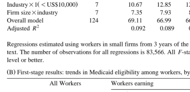
space, we cannot report all of these coefficients. Because of the large number of interactions, reporting selected coefficients is also problematic — the ‘‘main effects’’ of industry, firm size, and income are different for each state and each year, as are interactions among these variables. Therefore, we present our first-stage results in the following way: we report F-statistics for the various groups of variables and their interactions in Table 1A, and selected mean predicted values in Table 1B.
Not all of the state or industry fixed effects and the interactions are significantly different from zero, though F-statistics show that for each year each group of variables or interactions is statistically significant at conventional levels. The R2
statistics, which are 0.08 on average for the individual eligibility equations and 0.09 for the family eligibility equations, are reasonable considering that the first stage equations are estimated as linear probability models.9 Our first stage results
are summarized in a more meaningful way in Table 1B, which reports mean predicted values by year and earnings category for the two measures of Medicaid eligibility. The fitted values capture three important sources of variation in
Ž .
Medicaid eligibility two of which are evident in the table . First, since Medicaid is a joint state–federal program, in any year there are differences across states in the fraction of workers eligible for Medicaid. Second, as shown in the table, there is variation over time coming from the fact that federal and state legislation caused
Ž
Medicaid eligibility to increase over the time period covered by our data 1989 to
.
1995 . However, even in the later years the percentage of workers eligible themselves is quite low: 13.77% in 1995 as compared to 11.15% in 1989.10 The
family-based measure of Medicaid eligibility is higher in all years and has a slightly larger percentage point increase over the period. Third, within any state in any year, MU will vary across firms according to the degree to which they rely on low wage workers. This is seen by a comparison of the second and third column of Table 1B.
While the effect of the Medicaid expansions on employer decisions obviously
Ž
depends on how eligible workers are distributed across firms something that we
.
cannot observe in the CPS, and can only partially observe in our employer data , the low percentage of eligible workers overall gives a reason to suspect that any such effect was small. This is because a firm in which a significant majority of workers are ineligible for Medicaid is unlikely to drop or otherwise alter health benefits in response to the expansions, and low wage firms with a high fraction of
9Morrison 1972 shows that with a binary dependent variable, the RŽ . 2 is bounded below 1. We
investigated using a logit for the first-stage equation, however, the results were extremely similar to those of the linear probability model, and the logit complicated the estimation of the correct standard errors in the second stage.
10
Note that actual eligibility increased by more than the eligibility of this constant population due to
Ž .
workers who gained Medicaid eligibility via the expansions have always been less likely to offer insurance.
Table 1
Ž .A Fit statistics for first-stage regressions predicting Medicaid eligibility Independent variables Degrees of F-statistics
freedom 1989 1990 1991 1993 1995
DependentÕariable: own eligibility
State dummies 50 3.68 2.99 2.70 7.04 4.30
Ž .
State=1-US$10,000 50 9.06 5.53 5.40 8.27 5.74
Industry dummies 7 6.05 6.04 5.71 4.28 3.97
Ž .
Industry=1-US$10,000 7 11.53 17.22 16.94 20.82 19.12
Firm size=industry 7 7.90 10.06 9.80 10.71 9.63
Overall model 124 60.19 62.20 62.47 73.41 67.4
2
Adjusted R 0.081 0.083 0.085 0.097 0.090
DependentÕariable: family eligibility
State dummies 50 11.26 8.51 7.89 18.48 11.51
Ž .
State=1-US$10,000 50 6.64 3.68 3.66 4.02 3.94
Industry dummies 7 9.00 12.15 12.31 14.35 12.86
Ž .
Industry=1-US$10,000 7 10.67 12.85 12.26 14.17 12.14
Firm size=industry 7 7.35 7.93 8.01 8.55 7.63
Overall model 124 69.11 66.99 66.78 74.44 68.42
2
Adjusted R 0.092 0.089 0.089 0.098 0.091
Regressions estimated using workers in small firms from 3 years of the March CPS as described in the text. The number of observations for all regressions is 83,566. All F-statistics are significant at the 1% level or better.
Ž .B First-stage results: trends in Medicaid eligibility among workers, by income category All Workers Workers earning
-US$10,000ryear )US$10,000ryear Percentage of eligible for Medicaid
1989 11.15 19.31 3.85
1990 12.22 21.28 4.12
1991 12.24 21.64 4.23
1993 13.85 23.63 5.11
1995 13.77 23.58 5.01
Percentage in families with eligible members
1989 16.81 26.72 7.96
1990 18.66 29.59 8.90
1991 19.07 30.11 9.20
1993 21.24 32.47 11.22
1995 21.22 32.57 11.08
A final econometric issue with our two-sample technique pertains to the standard errors. In estimating the standard errors we treat the unobservability of
MfU as a missing data problem, and use a multiple imputations approach. A single
ˆ
X Ximputation is done by replacing M with M where M is a draw from the normal
ˆ
Ž .
distribution N M, sMˆ . A consistent estimate of the covariance matrix is TJ
where
˜
TJsVqB .J
Ž .
3˜
Ž .In this equation, V is the original uncorrected estimate of the covariance matrix and B isJ
J
1 X
BJs
Ý
ž
bybj/ ž
bybj/
Ž .
4Jy1js1
Ž .
where b is the coefficient vector from one of our Jj Js100 regressions using
X y1 11
M , a simulated value from the above distribution, and bj sJ Ýjb .j
4. The firm-level data
The firm-level data we use in our analysis were collected in five employer surveys conducted in 1989, 1990, 1991, 1993, and 1995. These surveys have been used individually and in various combinations in a number of published studies, and are perhaps the most widely cited source of information on employer health care costs and benefits. While the pooled cross-section data set we construct with
Ž .
these surveys is not without its weaknesses which we will discuss we are aware of no other available employer data set suitable for examining how employers may have responded to the Medicaid expansions.12
All of the surveys were administered by telephone to a sample of U.S. employers drawn from Dun and Bradstreet’s nationwide list of firms. The surveys
11 Ž .
Schenker and Welsh 1988 show the consistency of the multiple imputations estimator. For an
Ž .
application in a different context, see Brownstone and Valletta 1996 .
12
consist of two groups: the 1989–1991 surveys, sponsored by the Health Insurance
Ž .
Association of America HIAA , and the 1993 and 1995 surveys, sponsored by KPMGrPeat Marwick, the Robert Wood Johnson Foundation, and the Kaiser Family Foundation.13 Each of the HIAA surveys, which were intended to be nationally representative, contains between 2000 and 3300 observations on firms of all sizes. The 1993 and 1995 surveys were divided by firm size, with the large and small firm portions sponsored and conducted separately. Both the large and small firm samples consist of approximately 1000 firms in each year. Unfortu-nately, the large firm surveys from the later years contain data only for firms which offer insurance and do not include important questions pertaining to employee characteristics. In addition, the 1993 and 1995 samples include very few firms with one or two employees. In light of these problems, we restrict our analysis to firms with between 5 and 100 employees. While it would be ideal to have data on firms of all sizes, smaller firms are of particular interest, for three reasons. First, smaller firms are more likely to be making marginal decisions about whether or not to offer health insurance.14 Second, smaller firms are more likely to employ a homogenous workforce, and hence may be more likely to respond to the Medicaid expansions. Third, larger firms are more likely to operate in more than one state, making it difficult to relate Medicaid eligibility rules to firm behavior.
To ensure that our sample is nationally representative of firms in this size range, we obtained a measure of the distribution of firms by size and region from the Census Bureau’s County Business Patterns. To calculate firm-level weights, we divide the observations into categories based on year, Census region and five firm-size categories: 5–9 employees, 10–19, 20–49, and 50–99. The weight assigned to firms in each cell equals Pcrp , where P is the proportion of thec c
population represented by cell c, and p is the corresponding sample proportion.c
We also calculated a second set of weights to make the data nationally representa-tive with respect to employees in small firms. The employee-level weight assigned to an observation is the observation’s firm-level weight multiplied by the number of employees in the firm.
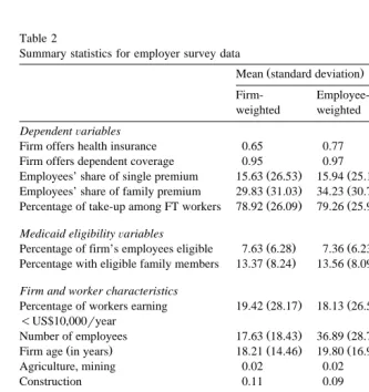
Table 2 presents firm-weighted and employee-weighted summary statistics from our firm level data. The top panel lists our dependent variables. The first is an indicator variable for whether or not the firm offers health insurance to its workers. As shown in Appendix A, the question on which this variable is based was essentially the same in each year. In the pooled sample, the firm-weighted
13 Ž .
The response rates were higher in the surveys conducted by HIAA between 66% and 70% than in
Ž .
the surveys of the two later years 44% and 58% .
14
mean is 0.65 and the employee-weighted mean is 0.77, the difference between the two reflecting the positive relationship between firm size and insurance provision. For firms that offer insurance we also examine various measures of plan generos-ity: whether or not the firm offers dependent coverage and the employee contribu-tions for single and family coverage, expressed as a percentage of the respective
Table 2
Summary statistics for employer survey data
Ž .
Mean standard deviation Minimum Maximum
Firm-
Employee-weighted weighted DependentÕariables
Firm offers health insurance 0.65 0.77 0 1
Firm offers dependent coverage 0.95 0.97 0 1
Ž . Ž .
Employees’ share of single premium 15.63 26.53 15.94 25.12 0 100
Ž . Ž .
Employees’ share of family premium 29.83 31.03 34.23 30.76 0 100
Ž . Ž .
Percentage of take-up among FT workers 78.92 26.09 79.26 25.91 1 100 Medicaid eligibilityÕariables
Ž . Ž .
Percentage of firm’s employees eligible 7.63 6.28 7.36 6.23 y1.69 42.10
Ž . Ž .
Percentage with eligible family members 13.37 8.24 13.56 8.09 y1.75 50.77 Firm and worker characteristics
Ž . Ž .
Percentage of workers earning 19.42 28.17 18.13 26.59 0 100
-US$10,000ryear
Ž . Ž .
Number of employees 17.63 18.43 36.89 28.71 5 100
Ž . Ž . Ž .
Firm age in years 18.21 14.46 19.80 16.96 0 215
Agriculture, mining 0.02 0.02 0 1
Construction 0.11 0.09 0 1
Manufacturing 0.14 0.18 0 1
Transportation, utilities 0.05 0.05 0 1
and communication
Wholesale trade 0.08 0.09 0 1
Retail trade 0.22 0.19 0 1
Finance, insurance, real estate 0.06 0.06 0 1
Services 0.31 0.30 0 1
County-leÕelÕariables
Ž . Ž . Ž .
Per capita income US$1000 20.67 0.61 20.67 0.58 8.12 58.10
Ž . Ž .
Unemployment rate 5.83 2.22 5.86 2.21 1.6 28.8
Ž . Ž .
Percentage of residents in poverty 12.62 5.81 12.70 5.76 2.6 47.5
Ž . Ž .
Percentage of residents in urban area 74.51 26.52 75.71 25.69 0 100
Ž . Ž .
Percentage of workers in manufacturing 17.36 7.51 17.50 7.55 1.1 51.7 Entries are summary statistics from 1989–1991 HIAA surveys and 1993 and 1995 KPMGrPeat MarwickrWayne State surveys. Summary statistics for explanatory variables pertain to the full sample
ŽNs3082 . Sample sizes for analyses limited to firms that offer insurance are smaller, and are.
premiums. As with insurance offers, the questions pertaining to these outcomes are nearly identical across the different surveys.
For firms that offer insurance we also examine the effect of Medicaid eligibility on employee take-up, though here there are some minor data problems. The HIAA surveys provide sufficient information to calculate the take-up rate among full-time employees who are offered benefits. While ideally we would like to know the take-up rate among all workers offered coverage, since part-time workers are seldom offered benefits, the distinction between all eligible workers and eligible full-time workers is not great.15 A second problem is that identical questions
pertaining to eligibility and take-up were not asked in the latter two surveys. It is possible, however, to use information on the total number of workers covered and yesrno questions on whether any part-time workers are offered insurance to
Ž
construct a close proxy for the take-up rate among full-time employees see
.
Appendix A for more details . Because the definition of this variable is not identical across all years, we also estimate a set of take-up regressions on the
Ž
1989–1991 sample only. Table 2 reports summary statistics on the take-up rate
.
for the entire 5 years. A final limitation of our data with respect to take-up is that since the establishment surveys provide no information on the number of workers who are married or have children, we cannot calculate a meaningful take-up rate for dependent coverage.
The next panel of Table 2 contains the Medicaid eligibility variables con-structed by combining coefficients estimated in the CPS with data from the employer surveys. The figures indicate that in the late 1980s to mid 1990s, most firms employed very few workers who either qualified for Medicaid or had family members who did. The firm-weighted sample means for the two variables are 7.63
Ž .
and 13.37, and the 75th percentile values not reported are 9.92 and 17.83, respectively.16
The firm characteristics common to all five employer surveys are firm size, firm age, the percent of workers earning less than US$10,000 per year, and industry. Since the data file for each year’s survey identifies the zip codes of responding firms we were able to determine the county in which each firm is located, and then merge in several county level-variables from the Area Resource File to control for local labor market conditions. Two of these variables — the county’s unemployment rate and per capita income — vary across counties and years, while the other three — the percentage of county residents in urban areas, the percent in poverty, and the percent employed in manufacturing — are based on the 1990 census, and hence vary only across county.
15 Ž .
According to the US Bureau of Labor Statistics 1994 , only 5% of part-time workers in firms with 100 or fewer employees received health benefits in 1992, compared to 71% of full-time workers.
16
5. Regression results
5.1. The firm’s decision to offer insurance
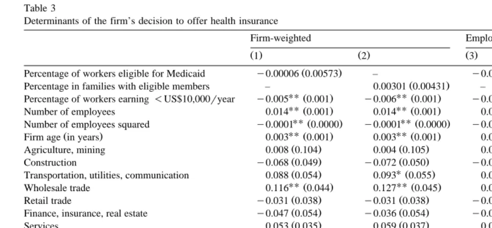
Table 3 presents results from several linear probability models of the firm’s decision to offer health insurance benefits.17 We report models using both
Medicaid eligibility variables and using firm- and employee-level weights. In a fully structural model, a firm’s decision to offer insurance will depend on the premiums it faces in the market. The estimation of such a model is compli-cated by the fact that premiums are observed only for those firms offering
Ž .
coverage see Feldman et al., 1997 . Since our interest is not in the effect of premiums per se, we estimate the model in the reduced form. As a result, the coefficients estimated for some variables combine an indirect effect working through their effect on premiums, as well as more direct effects. For example, our finding of a strong positive effect of firm size is at least partly explained by the fact that, ceteris paribus, smaller firms face higher premiums due to higher per-employee administrative costs.
Our results indicate that the probability of offering insurance increases by one percentage point for every 3 to 5 years that a firm has been in business. As with the firm size effect, this finding is consistent with results from other studies using
Ž .
establishment data Levy, 1997; Feldman et al., 1997 . The estimated coefficients on the county-level variables also conform with our expectations. Insurance provision is more common in counties with higher average income and less common in counties with higher poverty rates, though the latter effect is less precisely estimated. We find that health insurance provision is more common in
Ž
urban areas, a result that has been noted previously Markowitz et al., 1991;
.
Frenzen, 1993; Feldman et al., 1997; Coburn et al., 1998 . These significant county effects increase our confidence that our measures of Medicaid availability are not picking up unobserved factors related to local economic conditions.
Our results imply that firms that make greater use of low wage workers are significantly less likely to offer insurance. The firm-weighted results imply that a 10 percentage point increase in the percentage of workers earning less than US$10,000 per year lowers the offer probability by roughly 5 percentage points. Evaluated at the sample means, this corresponds to an elasticity of y0.15. The employee-weighted results are quite similar, translating to an elasticity ofy0.12. Because Medicaid is a means-tested program, this implies that firms with more Medicaid-eligible workers are less likely to offer insurance. However, this rela-tionship, in and of itself, does not bear directly on the question of crowd-out due
17
()
Determinants of the firm’s decision to offer health insurance
Firm-weighted Employee-weighted
Ž .1 Ž .2 Ž .3 Ž .4
Ž . Ž .
Percentage of workers eligible for Medicaid y0.00006 0.00573 – y0.00080 0.00468 –
Ž . Ž .
Percentage in families with eligible members – 0.00301 0.00431 – 0.00194 0.00349
UUŽ . UUŽ . UUŽ . UUŽ .
Percentage of workers earning-US$10,000ryear y0.005 0.001 y0.006 0.001 y0.005 0.001 y0.006 0.001
UUŽ . UUŽ . UUŽ . UUŽ .
Number of employees 0.014 0.001 0.014 0.001 0.010 0.001 0.010 0.001
UUŽ . UUŽ . UUŽ . UUŽ .
Number of employees squared y0.0001 0.0000 y0.0001 0.0000 y0.0001 0.0000 y0.0001 0.0000
UU UU UU UU
Ž . Ž . Ž . Ž . Ž .
Firm age in years 0.003 0.001 0.003 0.001 0.002 0.0004 0.002 0.0004
Ž . Ž . Ž . Ž .
Agriculture, mining 0.008 0.104 0.004 0.105 0.013 0.072 0.000 0.076
UU UU
Ž . Ž . Ž . Ž .
Construction y0.068 0.049 y0.072 0.050 y0.087 0.034 y0.088 0.034
U
Ž . Ž . Ž . Ž .
Transportation, utilities, communication 0.088 0.054 0.093 0.055 0.036 0.036 0.042 0.038
UUŽ . UUŽ . UUŽ . UUŽ .
Wholesale trade 0.116 0.044 0.127 0.045 0.067 0.028 0.077 0.029
Ž . Ž . Ž . Ž .
Retail trade y0.031 0.038 y0.031 0.038 y0.039 0.029 y0.036 0.029
Ž . Ž . Ž . Ž .
Finance, insurance, real estate y0.047 0.054 y0.036 0.054 y0.018 0.036 y0.007 0.036
Ž . Ž . Ž . Ž .
Services 0.053 0.035 0.059 0.037 0.017 0.022 0.022 0.023
UU UU
Ž . Ž . Ž . Ž . Ž .
Per capita income US$1000 0.006 0.002 0.006 0.002 0.003 0.002 0.003 0.002
Ž . Ž . Ž . Ž .
Unemployment rate 0.006 0.006 0.006 0.006 0.006 0.004 0.006 0.004
Ž . Ž . Ž . Ž .
Percentage of residents in poverty y0.003 0.003 y0.003 0.003 y0.002 0.002 y0.002 0.002
UUŽ . UUŽ . UUŽ . UUŽ .
Percentage of residents in urban area 0.001 0.0005 0.001 0.0005 0.001 0.0004 0.001 0.0004
Ž . Ž . Ž . Ž .
Percentage of workers in manufacturing y0.001 0.002 y0.001 0.002 y0.001 0.001 y0.001 0.001
2
R 0.269 0.269 0.273 0.273
Sample size 3062 3062 3062 3062
Ž .
Standard errors, corrected for two-step estimation method see text are in parentheses. All models include year and state dummy variables. UU
Statistically significant at the 0.05 level. U
to the expansions. Rather, it is the coefficients on our fitted Medicaid eligibility variables that provide tests of the hypothesis that the Medicaid expansions caused a reduction in insurance offers.18
In each of the four models, the estimated coefficient on the Medicaid variable is
Ž .
small and not significantly different from zero. In column 1 , the point estimate of
y0.00006 implies that a 10 percentage point increase in the percentage of a firm’s workers eligible for Medicaid will reduce the firm’s probability of offering insurance by less than one-tenth of one percentage point. At the employer-weighted sample means, this represents an elasticity of y0.0007. However, because the confidence interval around this estimate is fairly wide, we cannot rule out substantially larger effects. With a bootstrapped standard error of 0.0057, the
Ž .
lower bound of our 95% confidence interval i.e., the most negative effect implies that a 10 percentage point increase in Medicaid eligibility would lead to an 11
Ž
percentage point decline in the offer rate and the upper bound is a positive effect
.
of roughly the same magnitude . When we use the family-based measure of
Ž Ž ..
Medicaid eligibility and employer weights column 2 , the point estimate is positive, though the 95% confidence interval includes effects as negative as
y0.0059. The employee-weighted results are slightly more precise, though still statistically insignificant.
The finding that the expansions did not appear to affect the provision of insurance by small firms, although imprecisely estimated, is robust to changes in the way the Medicaid variables enter the regression. For instance, to examine whether there were effects of eligibility levels which were limited to firms with high levels of eligibility, we estimated models in which the percent eligible for Medicaid entered in categorical form.19 We tried a variety of categorizations;
none indicated a significant relationship between the availability of Medicaid for a firm’s employees and the decision to offer insurance. Models including the percent eligible squared also implied that any crowding-out that occurred as a result of the expansions was not caused by employers dropping coverage.
This finding is also robust to the inclusion or exclusion of key control variables. One possible criticism of the specifications reported in Table 3 is that by including a full set of state dummies in addition to the county variables, we may be ‘‘over-controlling’’ for local economic conditions and leaving too little residual variation to be explained by our Medicaid variable. To examine whether this was the case, we tried replacing the state dummies with dummies for the census region or division, which would increase the cross-sectional variation for identifying the crowd-out effect. Again, the results from such models were not qualitatively different from those reported in Table 3.
18
This point is illustrated by the fact that when we drop the percent under US$10,000 variable from the regression we obtain significant negative Medicaid effects.
19
Finally, an argument can be made that any negative effect of Medicaid eligibility on firm offer decisions may be limited to very small firms. To test this, we divided the sample into four equal-sized groups by firm size: firms with 10 or fewer employees, 11 to 25 employees, 26 to 50 employees, and more than 50 employees. We then re-estimated the models separately for each of the four groups, and found similar small, insignificant effects in all of them.
5.2. Measures of health plan generosity
Although we found no evidence that firms reduced their likelihood of offering coverage, some small insurance-providing firms may have responded to Medicaid
Ž
expansions by encouraging workers to enroll their children and perhaps
them-.
selves in the public program. The most direct way to do this is to drop family coverage altogether. A more subtle approach is to increase employee premium
Ž
contributions to encourage workers with Medicaid-eligible dependents and those
.
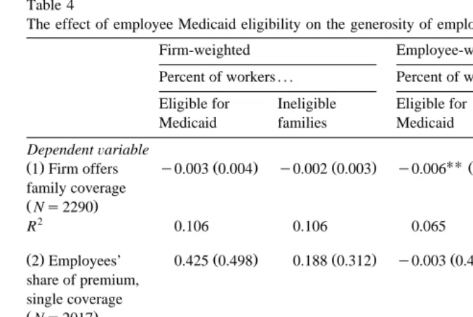
who are eligible themselves to voluntarily drop coverage. Table 4 reports the key results from regressions that attempt to investigate these potential effects. The column layout is similar to Table 3, though for the sake of brevity we do not report any control variable coefficients.20
The first row of Table 4 pertains to models in which the dependent variable equals one if the firm offers dependent coverage, and zero if insurance is offered to workers only. It is here that we find our strongest evidence of crowd-out. All four specifications reported yield a negative relationship between the fraction of a
Ž
firm’s employees estimated to be eligible for Medicaid or in families with eligible
.
members and the decision to offer family coverage. The effects are slightly larger and more precisely estimated when we weigh by the number of employees: the coefficients ofy0.006 andy0.004 in the third and fourth columns have absolute
t-statistics of 2.34 and 2.43, respectively. These effects are substantially larger
than those from the offer equations of Table 3. The point estimate from column 3
Žcolumn 4 implies that a 10 percentage point increase in the Medicaid eligibility. Ž .
variable decreases the probability of offering family coverage by 6 4 percentage
Ž .
points. At the lower most negative bound of our 95% confidence interval, a 10 point increase in Medicaid eligibility would correspond to a 12 percentage point decline in family offers.
The coefficients on most of the other variables in the row 1 model are statistically insignificant. In particular, the percent of low-wage workers in the firm does not affect the likelihood of a firm offering family coverage, conditional on offering coverage at all. The exceptions are that larger firms and ones that have been in business longer are more likely, and firms in urban areas are less likely, to
20
Table 4
The effect of employee Medicaid eligibility on the generosity of employer health benefit programs
Firm-weighted Employee-weighted
Percent of workers . . . Percent of workers . . . Eligible for Ineligible Eligible for Ineligible
Medicaid families Medicaid families
DependentÕariable
UU UU
Ž .1 Firm offers y0.003 0.004Ž . y0.002 0.003Ž . y0.006 Ž0.003. y0.004 Ž0.002.
family coverage
ŽNs2290.
2
R 0.106 0.106 0.065 0.065
Ž .2 Employees’ 0.425 0.498Ž . 0.188 0.312Ž . y0.003 0.402Ž . 0.075 0.268Ž .
share of premium, single coverage
ŽNs2017.
2
R 0.104 0.105 0.104 0.105
Ž .3 Employees’ 0.030 0.618Ž . y0.108 0.424Ž . y0.456 0.518Ž . y0.279 0.354Ž .
share of premium, family coverage
ŽNs1988.
2
R 0.183 0.183 0.177 0.177
UU
Statistically significant at the 0.05 level.
Ž .
Standard errors, corrected for two-step estimation method see text are in parentheses. Table entries are estimated coefficients of imputed Medicaid eligibility levels in regressions on the dependent variables noted above. All models include the same set of controls as in Table 3.
offer dependent coverage. Firms in mining and agriculture and finance, insurance, and real estate are somewhat more likely than manufacturing firms to offer family coverage, while firms in transportation and utilities are somewhat less likely. Differences across states are small and generally not statistically significant.
statisti-cally insignificant, with t-statistics less than one.21 When we use employee weights, the point estimates are much smaller, while the standard errors decline only slightly.
To the extent that employers did increase contributions in response to the availability of Medicaid, we would expect the effect to be greatest for family
Ž .
coverage. However, when we use percent family coverage contributions as our dependent variable, the Medicaid coefficients are substantially smaller than in the corresponding single coverage regressions. In fact, the employee-weighted coeffi-cient estimates are quite large and negative, though, again, insignificant due to large standard errors. Thus, while the imprecision of our results makes any definitive conclusion impossible, it is hard to rationalize the pattern of the point estimates with the hypothesis that employers’ premium contribution policies were influenced by the availability of Medicaid.22
In addition to these models, we also estimated regressions in which the dependent variable is the single or family contribution measured in dollars or as an indicator variable for whether any contribution is required at all. These additional regressions also offer no support for the hypothesis of a positive effect of Medicaid eligibility on the existence or level of employee premium contributions. However, as with the results reported in the table, the standard errors are quite large, which means we cannot rule out the possibility of fairly substantial effects.
5.3. Employee take-up
Regardless of how employers responded to the Medicaid expansions, private insurance may have fallen as a result of newly eligible workers declining coverage
Ž .
offered to them. As noted, the analysis by Cutler and Gruber 1996 using the CPS Employee Benefit Supplement suggests that this was the primary way that the expansions reduced private coverage. To address this possible effect, the final outcome we examine is the take-up rate among full-time employees who were offered insurance by their employers.
Because the take-up rate reflects decisions made by individual employees rather than employers, we estimate employment-weighted regressions only. The first two columns of Table 5 contain results for all firms in our sample that offer insurance. The next two columns contain results for a subsample of 966 firms that have 25 or more employees. There are two arguments for restricting the sample in this way. First, the fact that the take-up rate is observed only for firms that offer insurance
21
It is important to note that the dependent variable in row 1 is an indicator variable, whereas those
Ž .
in rows 2 and 3 range theoretically from 0 to 100. As a result, the coefficients are not directly comparable.
22
Since Medicaid eligibility increased most rapidly in the early part of our sample, we estimated the
Ž .
()
Take-up of private insurance by full-time employees, all years
All firms Firms with)25 employees Employee contribution required
Ž .1 Ž .2 Ž .3 Ž .4 Ž .5 Ž .6
Ž . Ž . Ž .
Percentage of workers y0.099 0.459 – y0.784 0.651 – y0.582 0.562 –
eligible for Medicaid
Ž . Ž . Ž .
Percentage in eligible – y0.218 0.286 – y0.555 0.380 – y0.512 0.339
families
UUŽ . UUŽ . UUŽ . UUŽ . UUŽ . UUŽ .
Employee premium y0.149 0.021 y0.149 0.021 y0.187 0.037 y0.187 0.037 y0.145 0.024 y0.145 0.024
Ž .
contribution single coverage
UUŽ . UUŽ . Ž . UUŽ . UŽ . UUŽ .
Percentage of workers y0.268 0.088 y0.242 0.068 y0.198 0.129 y0.223 0.100 y0.202 0.104 y0.201 0.080
earning-US$10,000ryear
Ž . Ž . Ž . Ž . Ž . Ž .
Number of employees 0.062 0.081 0.063 0.081 0.242 0.237 0.250 0.238 0.064 0.100 0.053 0.099
Ž . Ž . Ž . Ž . Ž . Ž .
Number of employees squared y0.0004 0.001 y0.0004 0.001 y0.002 0.002 y0.002 0.002 y0.001 0.001 y0.001 0.001
Ž . UUŽ . UUŽ . Ž . Ž . UUŽ . UUŽ .
Firm age in years 0.082 0.032 0.081 0.032 y0.033 0.037 y0.031 0.037 0.104 0.037 0.105 0.037
UU UU
Ž . Ž . Ž . Ž . Ž . Ž .
Agriculture, mining 2.879 3.727 4.059 3.979 3.700 5.065 5.243 5.436 10.188 4.676 11.991 4.859
UUŽ . UUŽ . UUŽ . UUŽ . Ž . Ž .
Construction y5.899 2.657 y5.773 2.673 y8.074 3.462 y7.991 3.458 y4.294 3.177 y4.038 3.181
Ž . Ž . Ž . Ž . Ž . Ž .
Transportation, utilities, y1.098 3.121 y1.547 3.120 1.498 4.173 0.952 4.190 0.297 3.826 y0.410 3.852
communication
Ž . Ž . Ž . Ž . Ž . Ž .
Wholesale trade y0.841 1.988 y1.534 2.048 y0.777 2.562 y1.499 2.712 0.636 2.356 y0.347 2.449
UUŽ . UUŽ . Ž . Ž . UUŽ . UUŽ .
Retail trade y5.308 2.755 y5.447 2.748 y7.706 5.339 y7.006 4.988 y7.594 3.514 y7.480 3.487
Ž . Ž . Ž . Ž . Ž . Ž .
Finance, insurance, 1.040 2.457 0.414 2.393 y2.220 3.623 y2.044 3.224 y1.114 3.033 y1.607 3.002
real estate
UUŽ . UUŽ . Ž . Ž . UUŽ . UUŽ .
Services y3.391 1.553 y3.862 1.623 y2.319 2.374 y3.190 2.540 y4.083 2.031 y5.032 2.158
Ž . Ž . Ž . Ž . Ž . Ž .
Per capita income 0.280 0.179 0.285 0.178 0.226 0.264 0.232 0.259 0.443 0.295 0.456 0.292
ŽUS$1000.
U U
Ž . Ž . Ž . Ž . Ž . Ž .
Unemployment rate 0.177 0.387 0.194 0.383 0.474 0.616 0.468 0.603 0.750 0.448 0.756 0.443
U U
Ž . Ž . Ž . Ž . Ž . Ž .
Percentage of y0.100 0.190 y0.104 0.190 y0.406 0.244 y0.404 0.243 y0.192 0.239 y0.186 0.237
residents in poverty
Ž . Ž . Ž . Ž . Ž . Ž .
Percentage of y0.002 0.029 y0.003 0.029 y0.008 0.039 y0.007 0.039 0.015 0.040 0.015 0.040
residents in urban area
Ž . Ž . Ž . Ž . Ž . Ž .
Percentage of 0.026 0.095 0.024 0.095 y0.200 0.141 y0.200 0.141 0.017 0.119 0.016 0.120
workers in manufacturing 2
R 0.200 0.200 0.279 0.280 0.232 0.233
Sample size 2050 2050 966 966 1421 1421
Ž .
Standard errors, corrected for two-step estimation method see text are in parentheses. All models include year and state dummy variables and are run using employee weights, as noted in the text. UU
Statistically significant at the 0.05 level. U
raises the issue of selectivity bias. Since as firm size increases it becomes less and less common for firms not to offer insurance, selectivity bias should be less of a problem for larger firms.23 The second argument is that the percent take-up rate will vary little, and is likely to be measured with substantial error, in very small firms.24 Since few workers will decline coverage when no premium contribution
Ž .
is required even if alternative coverage is available , we also estimate the take-up equation on a sample of 1421 firms that require a monthly premium contribution
Ž .
for either single or family coverage columns 5 and 6 .
The explanatory variables include those used in the other regressions plus the employee premium contribution required for the single coverage plan. While this variable is arguably endogenous, the results from Table 4 suggest that employer contribution policies are orthogonal to the availability of Medicaid. Because of this and the fact that it is an important determinant of employee take-up, we include
Ž
the employee contribution on the right hand side though dropping it has no
.
material effect on any of the other coefficients . As expected, the estimated effect of the premium contribution is negative and significant. Since the dependent variable is scaled from 0 to 100, the column 1 results imply that a US$10 increase in the monthly premium contribution reduces the employee take-up rate by 1.5 percentage points. Evaluated at the sample means for our data, the premium contribution coefficient from the full sample regression corresponds to an elastic-ity of y0.045, which is quite comparable to the take-up elasticity of y0.036
Ž .
calculated by Chernew et al. 1997 using a combined employer–employee data set.
Ž
Consistent with other studies using different types of data Chernew et al.,
.
1997; Cooper and Schone, 1997 the results in Table 5 indicate that the take-up rate declines with the percentage of low wage workers in the firm. Again, while workers earning less than US$10,000 are substantially more likely to qualify for Medicaid, this is not necessarily evidence of a negative impact of Medicaid, since it is difficult to disentangle the effects of Medicaid availability on demand for employer-provided insurance from other factors affecting insurance coverage for low-wage workers. It is, however, relevant to more general policy questions concerning the insurance coverage of low wage workers. For example, this result indicates that requiring firms to offer coverage to low-wage workers may not
23
An alternative approach to the issue of selection is to combine offering and non-offering firms to estimate models of ‘‘percent covered,’’ coding all non-offering firms as zeros. We estimated such models and they generated insignificant Medicaid effects. This result is not surprising given our results for the offer equations.
24
() Employee take-up results for HIAA data 1989 – 1991
All firms Firms with)25 employees Employee contribution required
Ž .1 Ž .2 Ž .3 Ž .4 Ž .5 Ž .6
Ž . Ž . Ž .
Percentage of workers y0.511 0.692 – y1.636 1.346 – y1.217 0.845 –
eligible for Medicaid
Employee premium y0.223 0.046 y0.223 0.046 y0.248 0.079 y0.247 0.080 y0.205 0.054 y0.205 0.054
Ž .
contribution single coverage
Ž . Ž . Ž . Ž . Ž . Ž .
Percentage of workers y0.172 0.119 y0.147 0.101 y0.062 0.232 y0.178 0.155 y0.066 0.148 y0.071 0.115
earning-US$10,000ryear
Ž . Ž . Ž . Ž . Ž . Ž .
Number of employees 0.065 0.101 0.056 0.101 0.227 0.297 0.239 0.299 0.071 0.148 0.046 0.149
Ž . Ž . Ž . Ž . Ž . Ž .
Number of employees squared y0.0004 0.001 y0.0004 0.001 y0.002 0.003 y0.002 0.003 y0.001 0.001 y0.001 0.001
U U UU UU
Ž . Ž . Ž . Ž . Ž . Ž . Ž .
Firm age in years 0.074 0.043 0.073 0.043 y0.051 0.053 y0.050 0.053 0.125 0.053 0.125 0.052
Ž . Ž . Ž . Ž . UŽ . UUŽ .
Agriculture, mining 3.875 4.475 6.089 5.245 4.971 8.128 5.848 9.126 10.409 5.589 13.848 6.211
UU UU
Ž . Ž . Ž . Ž . Ž . Ž .
Construction y3.464 3.136 y3.466 3.128 y6.670 3.193 y7.247 3.171 y3.745 3.887 y3.933 3.949
Ž . Ž . Ž . Ž . Ž . Ž .
Transportation, utilities, y1.202 3.710 0.183 3.879 y1.104 5.267 y1.114 5.538 0.589 5.542 y0.899 5.664
communication
Ž . Ž . Ž . Ž . Ž . Ž .
Wholesale trade y2.186 2.701 y3.347 2.963 y4.328 3.803 y4.003 4.026 y0.462 2.976 y2.028 3.152
U U
Ž . Ž . Ž . Ž . Ž . Ž .
Retail trade y5.043 3.634 y5.027 3.643 y12.465 7.771 y9.754 6.560 y8.077 4.917 y7.513 4.869
Ž . Ž . Ž . Ž . Ž . Ž .
Finance, insurance, y1.859 3.616 y2.537 3.518 y8.884 6.352 y6.540 5.195 y5.128 4.641 y5.434 4.469
real estate
UUŽ . UUŽ . Ž . Ž . UŽ . UUŽ .
Services y4.727 2.286 y5.578 2.490 y5.454 3.444 y5.909 3.825 y5.392 3.113 y6.809 3.381
Ž . Ž . Ž . Ž . Ž . Ž .
Per capita income 0.183 0.368 0.186 0.367 0.341 0.476 0.343 0.478 0.084 0.476 0.098 0.476
ŽUS$1000.
Ž . Ž . Ž . Ž . Ž . Ž .
Unemployment rate 0.313 0.492 0.293 0.493 0.041 0.767 0.043 0.760 0.427 0.744 0.398 0.742
U U
Ž . Ž . Ž . Ž . Ž . Ž .
Percentage of y0.179 0.215 y0.177 0.216 y0.330 0.237 y0.331 0.240 y0.456 0.257 y0.443 0.256
residents in poverty
Ž . Ž . Ž . Ž . Ž . Ž .
Percentage of y0.010 0.040 y0.010 0.040 y0.041 0.057 y0.045 0.057 y0.010 0.059 y0.008 0.060
residents in urban area
Ž . Ž . Ž . Ž . Ž . Ž .
Percentage of 0.057 0.141 0.055 0.141 y0.023 0.244 y0.020 0.223 y0.049 0.187 y0.054 0.187
workers in manufacturing 2
R 0.200 0.246 0.279 0.374 0.232 0.277
Sample size 1313 1313 646 646 874 874
Ž .
Standard errors, corrected for two-step estimation method see text are in parentheses. All models include year and state dummy variables and are run using employee weights, as noted in the text. UU
Statistically significant at the 0.05 level. U
increase coverage as much as desired, since low-wage workers appear less likely to accept coverage that is offered.
As with the other outcomes analyzed, our estimates of the effect of Medicaid eligibility on take-up are plagued by relatively large standard errors. However, for all models estimated, our point estimates imply a negative effect of Medicaid eligibility on the percentage of workers accepting offers of insurance, and the pattern of the results across the various subsamples is consistent with expectations. For example, the Medicaid eligibility coefficients are substantially larger in the sample that excludes very small firms than in the full sample. The column 4 results imply that a 10 percentage point increase in the percentage of workers in Medicaid-eligible families causes take-up to fall by 5.5 percentage points. With an absolute t-statistic of 1.47, this effect is significant at the 15% level. When we restrict the sample to firms that require employees to contribute directly for their
Ž .
coverage column 6 the coefficient on the family-based Medicaid variable is
Ž . Ž
approximately the same size y0.512 , with a similar significance level p-value
.
s0.13 .
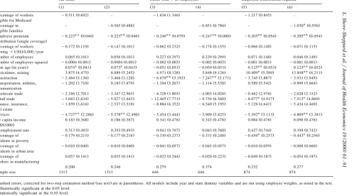
As noted above, our measure of take-up is clearly defined for the 1989, 1990, and 1991 surveys, and less clearly defined in the two later years. Consequently, we estimated the same models reported in Table 5 using only data from the three
Ž .
HIAA surveys 1989 to 1991 . The results from these regressions, which are reported in Table 6, also suggest a negative relationship between the percentage of workers in a firm who are eligible for Medicaid and the percentage of workers in the same firm who accept an offer of private coverage. In all cases, the Medicaid coefficients from these restricted samples are larger than their full-sample counter-parts. For example, when we drop the 1993 and 1995 data, the Medicaid coefficient for the column 2 specification goes fromy0.217 toy0.565. However, because the sample size falls from 2050 to 1313, the standard error on the
Ž .
coefficient also increases from 0.261 to 0.488 , yielding an absolute t-statistic of 1.16. Similarly, when we use only the 1989–1991 data and focus on firms that require premium contributions, we obtain a coefficient ofy1.030 on the
family-Ž .
based Medicaid coefficient standard errors0.556; absolute t-statistics1.85 .
Ž .
Taken together, these results provide some support albeit weak for the hypothesis that the Medicaid expansions crowded out private insurance by inducing some workers to decline offers of employer-sponsored insurance.
6. Conclusions
house-hold surveys have provided estimates of the magnitude of this crowd-out effect, because of the inherent limitations of the data used, they tell us little about the exact mechanisms by which it occurred. In particular, the previous literature sheds little light on the role of employers. A better understanding of this role is especially important as the further expansion of public programs causes more and more workers either to be eligible themselves or to have dependents who are eligible.
In this paper we use firm-level data collected over the period 1989 to 1995 to examine the role of firms in movements from private insurance to Medicaid. While the data we use are the best currently available for this type of investigation, they have important shortcomings which limit our analysis. Since the surveys we use were conducted for a different purpose, they provide no information on the Medicaid-eligibility status of workers employed by responding firms. To over-come this problem, we use a two-sample estimation strategy that combines the employer survey with data from the CPS. The use of this technique combined with a relatively small sample means that many of our estimated policy effects are quite imprecise. It is worth reiterating that the problem of imprecise estimates due to small sample sizes is not unique to our paper. This means that estimates of crowd-out from various papers may that appear to be widely divergent are often not statistically different from one another. Our results should be interpreted in this light.
With this caveat in mind, several results emerge from our analysis. First, while we find strong evidence that firms employing large fractions of low-wage workers are less likely to offer insurance, we find no evidence that the offer decision is affected by the percentage of a firm’s workers eligible for Medicaid. This result,
Ž .
which is consistent with the analysis by Cutler and Gruber 1996 using data from the Employee Benefit Supplement of the CPS, suggests that workers whose families remained ineligible for Medicaid did not lose insurance coverage as a result of the expansions. The absence of such a spillover effect implies that the cost of Medicaid crowd-out, whatever it may be, was not borne by employees of low wage firms who, for reasons of income or family status, do not qualify for Medicaid.