Sobolev Spaces on Lie Manifolds and
Regularity for Polyhedral Domains
Bernd Ammann, Alexandru D. Ionescu, Victor Nistor
Received: January 4, 2006 Revised: June 8, 2006
Communicated by Heinz Siedentop
Abstract. We study some basic analytic questions related to dif-ferential operators on Lie manifolds, which are manifolds whose large scale geometry can be described by a a Lie algebra of vector fields on a compactification. We extend to Lie manifolds several classical results on Sobolev spaces, elliptic regularity, and mapping properties of pseudodifferential operators. A tubular neighborhood theorem for Lie submanifolds allows us also to extend to regular open subsets of Lie manifolds the classical results on traces of functions in suitable Sobolev spaces. Our main application is a regularity result on poly-hedral domainsP⊂R3using the weighted Sobolev spacesKm
a(P). In
particular, we show that there is no loss ofKm
a –regularity for solutions
of strongly elliptic systems with smooth coefficients. For the proof, we identifyKm
a (P) with the Sobolev spaces onPassociated to the metric
r−P2gE, where gE is the Euclidean metric and rP(x) is a smoothing of the Euclidean distance from x to the set of singular points of P. A suitable compactification of the interior ofPthen becomes a regular open subset of a Lie manifold. We also obtain the well-posedness of a non-standard boundary value problem on a smooth, bounded do-main with boundaryO ⊂ Rn using weighted Sobolev spaces, where the weight is the distance to the boundary.
2000 Mathematics Subject Classification: 35J40 (Primary) 33J55, 35J70, 35J25, 47G30 (Secondary)
Contents
Introduction 162
1. Lie manifolds 166
1.1. Definition of Lie manifolds 166
1.2. Riemannian metric 168
1.3. Examples 168
1.4. V-differential operators 169
1.5. Regular open sets 169
1.6. Curvilinear polygonal domains 171
2. Submanifolds 173
2.1. General submanifolds 173
2.2. Second fundamental form 174
2.3. Tame submanifolds 175
3. Sobolev spaces 177
3.1. Definition of Sobolev spaces using vector fields and connections 178 3.2. Definition of Sobolev spaces using partitions of unity 180
4. Sobolev spaces on regular open subsets 184
5. A regularity result 190
6. Polyhedral domains in three dimensions 192
7. A non-standard boundary value problem 195
8. Pseudodifferential operators 197
8.1. Definition 197
8.2. Properties 198
8.3. Continuity onWs,p(M
0) 199
References 202
Introduction
We study some basic analytic questions on non-compact manifolds. In order to obtain stronger results, we restrict ourselves to “Lie manifolds,” a class of manifolds whose large scale geometry is determined by a compactification to a manifold with corners and a Lie algebra of vector fields on this compactification (Definition 1.3). One of the motivations for studying Lie manifolds is the loss of (classical Sobolev) regularity of solutions of elliptic equations on non-smooth domains. To explain this loss of regularity, let us recall first that the Poisson problem
(1) ∆u=f ∈Hm−1(Ω), m∈N∪ {0}, Ω⊂Rn bounded,
has a unique solutionu∈Hm+1(Ω),u= 0 on∂Ω, provided that∂Ωis smooth.
This well-posedness result is especially useful in practice for the numerical ap-proximation of the solution uof Equation (1) [8]. However, in practice, it is only rarely the case that Ω is smooth. The lack of smoothness of the domains interesting in applications has motivated important work on Lipschitz domains, see for instance [23, 40] or [65]. These papers have extended to Lipschitz do-mains some of the classical results on the Poisson problem on smooth, bounded domains, using the classical Sobolev spaces
Hm(Ω) :={u, ∂αu∈L2(Ω), |α| ≤m}.
It turns out that, if∂Ω isnotsmooth, then the smoothness off on Ω (i. e., up to the boundary) does not imply that the solutionuof Equation (1) is smooth as well on Ω. This is theloss of regularityfor elliptic problems on non-smooth domains mentioned above.
The loss of regularity can be avoided, however, by a conformal blowup of the singular points. This conformal blowup replaces a neighborhood of each con-nected component of the set of singular boundary points by a complete, but non-compact end. (Here “complete” means complete as a metric space, not geodesically complete.) It can be proved then that the resulting Sobolev spaces are the “Sobolev spaces with weights” considered for instance in [25, 26, 35, 46]. Letf >0 be a smooth function on a domain Ω, we then define themth Sobolev space with weight f by
(2) Km
a (Ω;f) :={u, f|α|−a∂αu∈L2(Ω), |α| ≤m}, m∈N∪ {0}, a∈R.
Indeed, if Ω =P⊂R2 is a polygon, and if we choose
(3) f(x) =ϑ(x) = thedistance to the non-smooth boundary points of P, then there is no loss of regularity in the spacesKm
a (Ω) :=Kma(Ω;ϑ) [26,
Theo-rem 6.6.1]. In this paper, we extend this regularity result to polyhedral domains in three dimensions, Theorem 6.1, with the same choice of the weight (in three dimensions the weight is the distance to the edges). The analogous result in arbitrary dimensions leads to topological difficulties [9, 66].
Our regularity result requires us first to study the weighted Sobolev spaces
Km
a(Ω) := Kma (Ω;ϑ) where ϑ(x) is the distance to the set of singular points
on the boundary. Our approach to Sobolev spaces on polyhedral domains is to show first that Km
a(Ω) is isomorphic to a Sobolev space on a certain
non-compact Riemannian manifold M with smooth boundary. This non-compact manifoldM is obtained from our polyhedral domain by replacing the Euclidean metricgE with
(4) r−P2gE, rP a smoothing ofϑ,
which blows up at the faces of codimension two or higher, that is, at the set of singular boundary points. (The metricrP−2gEis Lipschitz equivalent toϑ−2gE,
elements are vector fields onM. The spaceV must satisfy a number of axioms, in particular,V is required to be closed under the Lie bracket of vector fields. This property is the origin of the nameLie manifold. TheC∞(M)-moduleV
can be identified with the sections of a vector bundle Aover M. Choosing a metric on Adefines a complete Riemannian metric on the interior ofM. See Section 1 or [4] for details.
The framework of Lie manifolds is quite convenient for the study of Sobolev spaces, and in this paper we establish, among other things, that the main results on the classical Sobolev spaces remain true in the framework of Lie manifolds. The regular open sets of Lie manifolds then play in our framework the role played by smooth, bounded domains in the classical theory.
LetP⊂Rn be a polyhedral domain. We are especially interested in describing
the spacesKma−−1/21/2(∂P) of restrictions to the boundary of the functions in the weighted Sobolev space Km
a (P;ϑ) = Kam(P;rP) on P. Using the conformal change of metric of Equation (4), the study of restrictions to the boundary of functions in Km
a (P) is reduced to the analogous problem on a suitable regular
open subset ΩPof some Lie manifold. More precisely,Kam(P) =r a−n/2
P Hm(ΩP). A consequence of this is that
(5) Kma−−1/21/2(∂P) =Km−1/2
a−1/2(∂P;ϑ) =r a−n/2
P H
m−1/2(∂Ω
P). (In what follows, we shall usually simply denote Km
a(P) := Kma(P;ϑ) = Km
a(P;rP) and Kam(∂P) := Kam(∂P;ϑ) = Kma (∂P;rP), where, we recall, ϑ(x) is the distance from x to the set of non-smooth boundary points andrP is a smoothing ofϑthat satisfiesrP/ϑ∈[c, C],c, C >0.)
Equation (5) is one of the motivations to study Sobolev spaces on Lie manifolds. In addition to the non-compact manifolds that arise from polyhedral domains, other examples of Lie manifolds include the Euclidean spaces Rn, manifolds that are Euclidean at infinity, conformally compact manifolds, manifolds with cylindrical and polycylindrical ends, and asymptotically hyperbolic manifolds. These classes of non-compact manifolds appear in the study of the Yamabe problem [32, 48] on compact manifolds, of the Yamabe problem on asymptoti-cally cylindrical manifolds [2], of analysis on loasymptoti-cally symmetric spaces, and of the positive mass theorem [49, 50, 67], an analogue of the positive mass theo-rem on asymptotically hyperbolic manifolds [6]. Lie manifolds also appear in Mathematical Physics and in Numerical Analysis. Classes of Sobolev spaces on non-compact manifolds have been studied in many papers, of which we mention only a few [15, 18, 27, 30, 34, 36, 39, 37, 38, 51, 52, 53, 63, 64] in addition to the works mentioned before. Our work can also be used to unify some of the various approaches found in these papers.
Let us now review in more detail the contents of this paper. A large part of the technical material in this paper is devoted to the study of Sobolev spaces on Lie manifolds (with or without boundary). IfM is acompactmanifold with corners, we shall denote by ∂M the union of all boundary faces of M and by M0 :=
of a structural Lie algebra of vector fields V on a manifold with corners M. This Lie algebra of vector fields will provide the derivatives appearing in the definition of the Sobolev spaces. Then we define a Lie manifold as a pair (M,V), where M is a compact manifold with corners and V is a structural Lie algebra of vector fields that is unrestricted in the interior M0 of M. We
will explain the above mentioned fact that the interior ofM carries a complete metricg. This metric is unique up to Lipschitz equivalence (or quasi-isometry). We also introduce in this section Lie manifolds with (true) boundary and, as an example, we discuss the example of a Lie manifold with true boundary corresponding to curvilinear polygonal domains. In Section 2 we discuss Lie submanifolds, and most importantly, the global tubular neighborhood theorem. The proof of this global tubular neighborhood theorem is based on estimates on the second fundamental form of the boundary, which are obtained from the properties of the structural Lie algebra of vector fields. This property distinguishes Lie manifolds from general manifolds with boundary and bounded geometry, for which a global tubular neighborhood is part of the definition. In Section 3, we define the Sobolev spaces Ws,p(M
0) on the interior M0 of a
Lie manifold M, where either s ∈ N∪ {0} and 1 ≤ p ≤ ∞ or s ∈ R and 1< p <∞. We first define the spaces Ws,p(M
0),s∈N∪ {0}and 1≤p≤ ∞,
by differentiating with respect to vector fields in V. This definition is in the spirit of the standard definition of Sobolev spaces on Rn. Then we prove that there are two alternative, but equivalent ways to define these Sobolev spaces, either by using a suitable class of partitions of unity (as in [54, 55, 62] for example), or as the domains of the powers of the Laplace operator (for p= 2). We also consider these spaces on open subsets Ω0 ⊂M0. The spaces
Ws,p(M
0), for s ∈ R, 1 < p < ∞ are defined by interpolation and duality
or, alternatively, using partitions of unity. In Section 4, we discuss regular open subsets Ω⊂M. In the last two sections, several of the classical results on Sobolev spaces on smooth domains were extended to the spacesWs,p(M
0).
These results include the density of smooth, compactly supported functions, the Gagliardo-Nirenberg-Sobolev inequalities, the extension theorem, the trace theorem, the characterization of the range of the trace map in the Hilbert space case (p= 2), and the Rellich-Kondrachov compactness theorem.
In Section 5 we include as an application a regularity result for strongly el-liptic boundary value problems, Theorem 5.1. This theorem gives right away the following result, proved in Section 6, which states that there is no loss of regularity for these problems within weighted Sobolev spaces.
Theorem0.1. LetP⊂R3be a polyhedral domain andP be a strongly elliptic,
second order differential operator with coefficients in C∞(P). Letu∈ K1 a+1(P),
u= 0 on ∂P, a ∈R. If P u ∈ Km−1
a−1(P), then u∈ K m+1
a+1(P) and there exists
C >0 independent ofusuch that
kukKm+1 a+1(P)≤C
¡
kP ukKm−1
a−1(P)+kukK 0 a+1(P)
¢
, m∈N∪ {0}.
Note that the above theorem does not constitute a Fredholm (or normal solv-ability) result, because the inclusionKm+1
a+1(P)→ K0a+1(P) isnot compact. See
also [25, 26, 35, 46] and the references therein for similar results.
In Section 7, we obtain a “non-standard boundary value problem” on a smooth domainOin weighted Sobolev spaces with weight given by the distance to the boundary. The boundary conditions are thus replaced by growth conditions. Finally, in the last section, Section 8, we obtain mapping properties for the pseudodifferential calculus Ψ∞
V(M) defined in [3] between our weighted Sobolev
spacesρsWr,p(M). We also obtain a general elliptic regularity result for elliptic
pseudodifferential operators in Ψ∞ V(M).
Acknowledgements: We would like to thank Anna Mazzucato and Robert Lauter for useful comments. The first named author wants to thank MSRI, Berkeley, CA for its hospitality.
1. Lie manifolds
As explained in the Introduction, our approach to the study of weighted Sobolev spaces on polyhedral domains is based on their relation to Sobolev spaces on Lie manifolds with true boundary. Before we recall the definition of a Lie manifold and some of their basic properties, we shall first look at the following example, which is one of the main motivations for the theory of Lie manifolds.
Example 1.1. Let us take a closer look at the local structure of the Sobolev spaceKm
a (P) associated to a polygonP(recall (2)). Consider Ω :={(r, θ)|0<
θ < α}, which models an angle of P. Then the distance to the vertex is simplyϑ(x) =r, and theweighted Sobolev spacesassociated to Ω,Km
a (Ω), can
alternatively be described as (6) Km
a (Ω) =Kam(Ω;ϑ) :={u∈L2loc(Ω), r−a(r∂r)i∂θju∈L2(Ω), i+j≤m}.
The point of the definition of the spaces Km
a (Ω) was the replacement of the
local basis{r∂x, r∂y}with the local basis{r∂r, ∂θ} that is easier to work with
on the desingularization Σ(Ω) := [0,∞)×[0, α]∋(r, θ) of Ω. By further writing r =et, the vector field r∂
r becomes ∂t. Sincedt =r−1dr, the space K1m(Ω)
then identifies withHm(R
t×(0, α)). The weighted Sobolev spaceKm1(Ω) has
thus become a classical Sobolev space on the cylinder R×(0, α), as in [25]. The aim of the following definitions is to define such a desingularisation in general. The desingularisation will carry the structure of a Lie manifold, defined in the next subsection.
We shall introduce a further, related definition, namely the definition of a “Lie submanifolds of a Lie manifold” in Section 4.
1.1. Definition of Lie manifolds. At first, we want to recall the definition of manifolds with corners. A manifold with corners is a closed subset M of a differentiable manifold such that every point p ∈ M lies in a coordinate chart whose restriction toM is a diffeomorphism to [0,∞)k×Rn−k, for some
that the transition map of two different charts are smooth up to the boundary. Ifk= 0 for allp∈M, we shall say thatM is asmooth manifold. Ifk∈ {0,1}, we shall say thatM is a smooth manifold with smooth boundary.
LetM be acompactmanifold with corners. We shall denote by∂M the union of all boundary faces ofM, that is,∂M is the union of all points not having a neighborhood diffeomorphic toRn. Furthermore, we shall writeM0:=Mr∂M for the interiorof M. In order to avoid confusion, we shall use this notation and terminology only whenM is compact. Note that our definition allows∂M to be a smooth manifold, possibly empty.
As we shall see below, a Lie manifold is described by a Lie algebra of vector fields satisfying certain conditions. We now discuss some of these conditions. Definition 1.2. A subspaceV ⊆Γ(M;T M) of the Lie algebra of all smooth vector fields onM is said to be astructural Lie algebra of vector fields onM provided that the following conditions are satisfied:
(i) V is closed under the Lie bracket of vector fields;
(ii) everyV ∈ V is tangent to all boundary hyperfaces ofM; (iii) C∞(M)V=V; and
(iv) each pointp∈M has a neighborhoodUp such that VUp:={X|Up|X∈ V} ≃C∞(Up)k
in the sense ofC∞(U
p)-modules.
The condition (iv) in the definition above can be reformulated as follows: (iv’) For every p∈M, there exist a neighborhoodUp ⊂M of pand vector
fields X1, X2, . . . , Xk ∈ V with the property that, for any Y ∈ V, there
exist functions f1, . . . , fk ∈ C∞(M), uniquely determined on Up, such
that
(7) Y =
k
X
j=1
fjXj onUp.
We now have defined the preliminaries for the following important definition. Definition1.3. ALie structure at infinityon a smooth manifoldM0is a pair
(M,V), where M is a compact manifold with interiorM0 andV ⊂Γ(M;T M)
is a structural Lie algebra of vector fields onM with the following property: If p∈M0, then any local basis ofV in a neighborhood of pis also a local basis
of the tangent space to M0.
It follows from the above definition that the constantkof Equation (7) equals to the dimensionnofM0.
A manifold with a Lie structure at infinity (or, simply, a Lie manifold) is a manifoldM0together with a Lie structure at infinity (M,V) onM0. We shall
sometimes denote a Lie manifold as above by (M0, M,V), or, simply, by (M,V),
becauseM0is determined as the interior ofM. (In [4], only the term “manifolds
Example 1.4. IfF ⊂T M is a sub-bundle of the tangent bundle of a smooth manifold (so M has no boundary) such that VF := Γ(M;F) is closed under
the Lie bracket, thenVF is a structural Lie algebra of vector fields. Using the
Frobenius theorem it is clear that such vector bundles are exactly the tangent bundles of k-dimensional foliations on M,k= rankF. However,VF does not
define a Lie structure at infinity, unlessF =T M.
Remark 1.5. We observe that Conditions (iii) and (iv) of Definition 1.2 are equivalent to the condition that V be a projectiveC∞(M)-module. Thus, by
the Serre-Swan theorem [24], there exists a vector bundleA→M, unique up to isomorphism, such that V = Γ(M;A). Since V consists of vector fields, that is V ⊂ Γ(M;T M), we also obtain a natural vector bundle morphism ̺M :A→T M, called theanchor map. The Condition (ii) of Definition 1.3 is
then equivalent to the fact that ̺M is an isomorphism A|M0 ≃ T M0 on M0.
We will take this isomorphism to be an identification, and thus we can say that Aisan extension ofT M0 toM (that is,T M0⊂A).
1.2. Riemannian metric. Let (M0, M,V) be a Lie manifold. By definition, a
Riemannian metric on M0 compatible with the Lie structure at infinity (M,V)
is a metric g0 on M0 such that, for any p ∈ M, we can choose the basis
X1, . . . , Xk in Definition 1.2 (iv’) (7) to be orthonormal with respect to this
metric everywhere on Up∩M0. (Note that this condition is a restriction only
for p ∈ ∂M := M rM0.) Alternatively, we will also say that (M0, g0) is a
Riemannian Lie manifold. Any Lie manifold carries a compatible Riemannian metric, and any two compatible metrics are bi-Lipschitz to each other.
Remark 1.6. Using the language of Remark 1.5,g0 is a compatible metric on
M0if, and only if, there exists a metricg on the vector bundleA→M which
restricts tog0 onT M0⊂A.
The geometry of a Riemannian manifold (M0, g0) with a Lie structure (M,V)
at infinity has been studied in [4]. For instance, (M0, g0) is necessarily complete
and, if ∂M 6= ∅, it is of infinite volume. Moreover, all the covariant deriva-tives of the Riemannian curvature tensor are bounded. Under additional mild assumptions, we also know that the injectivity radius is bounded from below by a positive constant, i. e., (M0, g0) is of bounded geometry. (Amanifold with
bounded geometry is a Riemannian manifold with positive injectivity radius and with bounded covariant derivatives of the curvature tensor, see [54] and references therein).
On a Riemannian Lie manifold (M0, M,V, g0), the exponential map exp :
T M0 → M0 is well-defined for all X ∈ T M0 and extends to a differentiable
map exp :A→M. A convenient way to introduce the exponential map is via the geodesic spray, as done in [4]. Similarly, any vector fieldX ∈ V = Γ(M;A) is integrable and will map any (connected) boundary face ofM to itself. The resulting diffeomorphism ofM0 will be denotedψX.
Examples 1.7.
(a) TakeVbto be the set of all vector fields tangent to all faces of a manifold
with corners M. Then (M,Vb) is a Lie manifold. This generalizes
Example 1.1. See also Subsection 1.6 and Section 6. Letr≥0 to be a smooth function onM that is equal to the distance to the boundary in a neighborhood of∂M, and is>0 outside∂M (i. e., onM0). Let hbe
a smooth metric onM, theng0=h+ (r−1dr)2 is a compatible metric
onM0.
(b) Take V0 to be the set of all vector fields vanishing on all faces of a
manifold with cornersM. Then (M,V0) is a Lie manifold. If∂M is a
smooth manifold (i. e., ifM is a smooth manifold with boundary), then
V0=rΓ(M;T M), where ris as in (a).
1.4. V-differential operators. We are especially interested in the analysis of the differential operators generated using only derivatives inV. Let Diff∗V(M)
be the algebra of differential operators onM generated by multiplication with functions in C∞(M) and by differentiation with vector fields X ∈ V. The
space of ordermdifferential operators in Diff∗V(M) will be denoted DiffmV(M).
A differential operator in Diff∗V(M) will be called a V-differential operator.
We can defineV-differential operators acting between sections of smooth vector bundlesE, F →M,E, F ⊂M×CN by
(8) Diff∗V(M;E, F) :=eFMN(Diff∗V(M))eE,
whereMN(Diff∗V(M)) is the algebra ofN×N-matrices over the ring Diff∗V(M),
and whereeE, eF ∈MN(C∞(M)) are the projections ontoEand, respectively,
ontoF. It follows that Diff∗V(M;E) := Diff∗V(M;E, E) is an algebra. It is also
closed under taking adjoints of operators inL2(M
0), where the volume form is
defined using a compatible metricg0 onM0.
1.5. Regular open sets. We assume from now on thatrinj(M0), the
injec-tivity radius of(M0, g0), is positive.
One of the main goals of this paper is to prove the results on weighted Sobolev spaces on polyhedral domains that are needed for regularity theorems. We shall do that by reducing the study of weighted Sobolev spaces to the study of Sobolev spaces on “regular open subsets” of Lie manifolds, a class of open sets that plays in the framework of Lie manifolds the role played by domains with smooth boundaries in the framework of bounded, open subsets ofRn. Regular open subsets are defined below in this subsection.
LetN ⊂M be a submanifold of codimension one of the Lie manifold (M,V). Note that this implies thatN is a closed subset ofM. We shall say that N is aregularsubmanifold of (M,V) if we can choose a neighborhoodV ofN inM and a compatible metric g0 on M0 that restricts to a product-type metric on
V ∩M0 ≃(∂N0)×(−ε0, ε0), N0=Nr∂N =N∩M0. Such neighborhoods
will be calledtubular neighborhoods.
and sufficient condition for the regularity of a codimension one submanifold of M. This is relevant, since the study of manifolds with boundary and bounded geometry presents some unexpected difficulties [47].
In the following, it will be important to distinguish properly between the bound-ary of a topological subset, denoted by∂top, and the boundary in the sense of
manifolds with corners, denoted simply by∂.
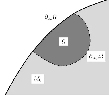
Definition1.8. Let (M,V) be a Lie manifold and Ω⊂M be an open subset. We shall say that Ω is a regular open subset in M if, and only if, Ω is con-nected, Ω and Ω have the same boundary,∂topΩ (in the sense of subsets of the
topological spaceM), and∂topΩ is a regular submanifold ofM.
Let Ω ⊂ M be a regular open subset. Then Ω is a compact manifold with corners. The reader should be aware of the important fact that∂topΩ =∂topΩ is
contained in∂Ω, but in general∂Ω and∂topΩ are not equal. The set∂topΩ will
be called thetrue boundaryof Ω. Furthermore, we introduce∂∞Ω :=∂Ω∩∂M,
and call it theboundary at infinityof Ω. Obviously, one has∂Ω =∂topΩ∪∂∞Ω.
The true boundary and the boundary at infinity intersect in a (possibly empty) set of codimension ≥2. See Figure 1. We will also use the notation ∂Ω0 :=
∂topΩ∩M0=∂Ω∩M0.
Ω
∂topΩ
∂∞Ω
M0
Figure 1. A regular open set Ω. Note that the interior of ∂∞Ω is contained in Ω, but the true boundary∂topΩ =∂topΩ
is not contained in Ω
The space of restrictions to Ω or Ω of ordermdifferential operators in Diff∗V(M)
will be denoted DiffmV(Ω), respectively DiffmV(Ω). Similarly, we shall denote by
V(Ω) the space of restrictions to Ω of vector fields in V, the structural Lie algebra of vector fields onM.
vector fields in V toF are tangent toF. However, ifF ⊂∂topΩ the regularity
of the boundary implies that there are vector fields in V whose restriction to F is not tangent toF. In particular, the true boundary∂topΩ of Ω is uniquely
determined by (Ω,V(Ω)), and hence so is Ω = Ωr∂topΩ. We therefore obtain a one-to-one correspondence between Lie manifolds with true boundary and regular open subsets (of some Lie manifoldM).
Assume we are given Ω, Ω (the closure inM), andV(Ω), with Ω a regular open subset of some Lie manifold (M,V). In the cases of interest, for example if ∂topΩ is a tame submanifold ofM (see Subsection 2.3 for the definition of tame
submanifolds), we can replace the Lie manifold (M,V) in which Ω is a regular open set with a Lie manifold (N,W) canonically associated to (Ω,Ω,V(Ω)) as follows. LetN be obtained by gluing two copies of Ω along∂topΩ, the so-called
double of Ω, also denoted Ωdb = N. A smooth vector field X on Ωdb will be in W, the structural Lie algebra of vector fields W on Ωdb if, and only if, its restriction to each copy of Ω is in V(Ω). Then Ω will be a regular open set of the Lie manifold (N,W). For this reason, the pair (Ω,V(Ω)) will be called a Lie manifold with true boundary. In particular, the true boundary of a Lie manifold with true boundary is a tame submanifold of the double. The fact that the double is a Lie manifold is justified in Remark 2.10.
1.6. Curvilinear polygonal domains. We conclude this section with a dis-cussion of a curvilinear polygonal domain P, an example that generalizes Ex-ample 1.1 and is one of the main motivations for considering Lie manifolds. To study function spaces onP, we shall introduce a “desingularization” (Σ(P), κ) of P (or, rather, of P), where Σ(P) is a compact manifold with corners and κ: Σ(P)→P is a continuous map that is a diffeomorphism from the interior of Σ(P) toPand maps the boundary of Σ(P) onto the boundary ofP.
Let us denote byBk the open unit ball inRk.
Definition 1.9. An open, connected subset P ⊂ M of a two dimensional manifoldM will be called acurvilinear polygonal domainif, by definition,Pis compact and for every pointp∈∂Pthere exists a diffeomorphismφp:Vp→B2, φp(p) = 0, defined on a neighborhoodVp⊂M such that
(9) φj(Vp∩P) ={(rcosθ, rsinθ), 0< r <1,0< θ < αp}, αp∈(0,2π).
A pointp∈∂Pfor whichαp6=πwill be called avertex of P. The other points of ∂Pwill be called smooth boundary points. It follows that every curvilinear polygonal domain has finitely many vertices and its boundary consists of a finite union of smooth curves γj (called the edgesof P) which have no other
common points except the vertices. Moreover, every vertex belongs to exactly two edges.
Let{P1, P2, . . . , Pk} ⊂Pbe the vertices of P. The casesk= 0 and k= 1 are
also allowed. Let Vj :=VPj andφj :=φPj :Vj →B2 be the diffeomorphisms
defined by Equation (9). Let (r, θ) : R2r{(0,0)} → (0,∞)×[0,2π) be the polar coordinates. We can assume that the sets Vj are disjoint and define
ThedesingularizationΣ(P) ofPwill replace each of the verticesPj,j= 1, . . . , k of P with a segment of length αj = αPj >0. Assume that P ⊂R2. We can realize Σ(P) inR3as follows. Letψjbe smooth functions supported onVjwith ψj= 1 in a neighborhood ofPj.
Φ :P r{P1, P2, . . . , Pk} →R2×R, Φ(p) =¡p ,X
j
ψj(p)θj(p)
¢
.
Then Σ(P) is (up to a diffeomorphism) the closure of Φ(P) inR3. The
desin-gularization map isκ(p, z) =p.
The structural Lie algebra of vector fieldsV(P) on Σ(P) is given by (the lifts of) the smooth vector fieldsX onP r{P1, P2, . . . , Pk}that, onVj, can be written as
X=ar(rj, θj)rj∂rj +aθ(rj, θj)∂θj,
witharandaθsmooth functions of (rj, θj),rj≥0. Then (Σ(P),V(P)) is a Lie
manifold with true boundary.
To define the structural Lie algebra of vector fields on Σ(P), we now choose a smooth function rP :P→[0,∞) with the following properties
(i) rP is continuous onP, (ii) rP is smooth onP,
(iii) rP(x)>0 on P r{P1, P2, . . . , Pk},
(iv) rP(x) =rj(x) ifx∈Vj.
Note that rP lifts to a smooth positive function on Σ(P). Of course, rP is determined only up to a smooth positive function ψon Σ(P) that equals to 1 in a neighborhood of the vertices.
Definition 1.10. A function of the formψrP, withψ∈ C∞(Σ(P)),ψ >0 will be called acanonical weight function of P.
In what follows, we can replacerPwith any canonical weight function. Canon-ical weight functions will play an important role again in Section 6. Canoni-cal weights are example of “admissible weights,” which will be used to define weighted Sobolev spaces.
Then an alternative definition ofV(P) is
(10) V(P) :={rP(ψ1∂1+ψ2∂2)}, ψ1, ψ2∈ C∞(Σ(P)).
Here∂1denotes the vector field corresponding to the derivative with respect to
the first component. The vector field∂2 is defined analogously. In particular,
(11) rP(∂jrP) =rP ∂rP ∂xj
∈ C∞(Σ(P)),
which is useful in establishing thatV(P) is a Lie algebra. Also, let us notice that both{rP∂1, rP∂2}and{rP∂rP, ∂θ}are local bases forV(P) onVj. The transition functions lift to smooth functions on Σ(P) defined in a neighborhood ofκ−1(Pj), but cannot be extended to smooth functions defined in a neighborhood of Pj
Then∂topΣ(P), the true boundary of Σ(P), consists of the disjoint union of the
edges ofP(note that the interiors of these edges have disjoint closures in Σ(P)). Anticipating the definition of a Lie submanifold in Section 2, let us notice that ∂topΣ(P) is a Lie submanifold, where the Lie structure consists of the vector
fields on the edges that vanish at the end points of the edges. The functionϑused to define the Sobolev spacesKm
a (P) :=Kma (P;ϑ) in
Equa-tion (2) is closely related to the funcEqua-tionrP. Indeed,ϑ(x) is the distance from x to the vertices of P. Therefore ϑ/rP will extend to a continuous, nowhere vanishing function on Σ(P), which shows that
(12) Km
a (P;ϑ) =Kma (P;rP).
If P is an order m differential operator with smooth coefficients on R2 and P ⊂ R2 is a polygonal domain, thenrm
P P ∈ Diff
m
V(Σ(P)), by Equation (10).
However, in general, rm
P P will not define a smooth differential operator onP. 2. Submanifolds
In this section we introduce various classes of submanifolds of a Lie manifold. Some of these classes were already mentioned in the previous sections.
2.1. General submanifolds. We first introduce the most general class of submanifolds of a Lie manifold.
We first fix some notation. Let (M0, M,V) and (N0, N,W) be Lie manifolds.
We know that there exist vector bundles A → M and B → N such that
V ≃ Γ(M;A) andW ≃ Γ(N;B), see Remark 1.5. We can assume that V = Γ(M;A) andW= Γ(N;B) and write (M, A) and (N, B) instead of (M0, M,V)
and (N0, N,W).
Definition 2.1. Let (M, A) be a Lie manifold with anchor map ̺M : A →
T M. A Lie manifold (N, B) is called aLie submanifoldof (M, A) if
(i) N is a closed submanifold ofM (possibly with corners, no transversality at the boundary required),
(ii) ∂N =N∩∂M (that is,N0⊂M0,∂N ⊂∂M), and
(iii) B is a sub vector bundle ofA|N, and
(iv) the restriction of ̺M toB is the anchor map ofB→N.
Remark 2.2. An alternative form of Condition (iv) of the above definition is (13) W= Γ(N;B) ={X|N|X∈Γ(M;A) andX|N tangent toN}
={X ∈Γ(N;A|N)|̺M ◦X ∈Γ(N;T N)}.
We have the following simple corollary that justifies Condition (iv) of Defini-tion 2.1.
Corollary 2.3. Let g0 be a metric onM0 compatible with the Lie structure
at infinity on M0. Then the restriction of g0 toN0 is compatible with the Lie
Proof. Letgbe a metric onAwhose restriction toT M0 defines the metricg0.
Theng restricts to a metric honB, which in turn defines a metrich0 onN0.
By definition,h0 is the restriction ofg0 toN0. ¤
We thus see that any submanifold (in the sense of the above definition) of a Riemannian Lie manifold is itself a Riemannian Lie manifold.
2.2. Second fundamental form. We define theA-normal bundleof the Lie submanifold (N, B) of the Lie manifold (M, A) as νA = (A|
N)/B which is a
bundle over N. Then the anchor map̺M defines a map νA →(T M|N)/T N,
called theanchor map of νA, which is an isomorphism overN 0.
We denote the Levi-Civita-connection onAby∇Aand the Levi-Civita
connec-tion onB by∇B [4]. LetX, Y, Z∈ W= Γ(N;B) and ˜X,Y ,˜ Z˜∈ V = Γ(M;A)
be such thatX = ˜X|N, Y = ˜Y|N, Z = ˜Z|N. Then∇AX˜Y˜|N depends only on
X, Y ∈ W= Γ(N;B) and will be denoted∇A
XY in what follows. Furthermore,
the Koszul formula gives 2g( ˜Z,∇A
˜
YX˜) =∂̺M( ˜X)g( ˜Y ,Z˜) +∂̺M( ˜Y)g( ˜Z,X˜)−∂̺M( ˜Z)g( ˜X,Y˜) −g([ ˜X,Z˜],Y˜)−g([ ˜Y ,Z],˜ X)˜ −g([ ˜X,Y˜],Z),˜ 2g(Z,∇BYX) =∂̺M(X)g(Y, Z) +∂̺M(Y)g(Z, X)−∂̺M(Z)g(X, Y)
−g([X, Z], Y)−g([Y, Z], X)−g([X, Y], Z).
As this holds for arbitrary sectionsZof Γ(N;B) with extensions ˜Zon Γ(M;A), we see that ∇B
XY is the tangential part of∇AXY|N.
The normal part of ∇A then gives rise to the second fundamental form II
defined as
II :W × W →Γ(νA), II(X, Y) :=∇AXY − ∇BXY.
The Levi-Civita connections∇A and∇B are torsion free, and hence II is
sym-metric because
II(X, Y)−II(Y, X) = [ ˜X,Y˜]|N−[X, Y] = 0.
A direct computation reveals also that II(X, Y) is tensorial in X, and hence, because of the symmetry, it is also tensorial in Y. (“Tensorial” here means II(f X, Y) = fII(X, Y) = II(X, f Y), as usual.) Therefore the second funda-mental form is a vector bundle morphism II :B⊗B→νA, and the
endomor-phism at p∈M is denoted by IIp : Bp⊗Bp → Ap. It then follows from the
compactness of N that
kIIp(Xp, Yp)k ≤CkXpk kYpk,
with a constant C independent of p∈ N. Clearly, on the interiorN0 ⊂M0
the second fundamental form coincides with the classical second fundamental form.
Corollary 2.4. Let (N, B) be a submanifold of (M, A) with a compatible metric. Then the (classical) second fundamental form ofN0inM0is uniformly
2.3. Tame submanifolds. We now introduce tame manifolds. Our main in-terest in tame manifolds is the global tubular neighborhood theorem, Theorem 2.7, which asserts that a tame submanifold of a Lie manifold has a tubular neighborhood in a strong sense. In particular, we will obtain that a tame sub-manifold of codimension one is regular. This is interesting because being tame is an algebraic condition that can be easily verified by looking at the structural Lie algebras of vector fields. On the other hand, being a regular submanifold is an analytic condition on the metric that may be difficult to check directly. Definition 2.5. Let (N, B) be a Lie submanifold of the Lie manifold (M, A) with anchor map̺M :A→T M. Then (N, B) is called atame submanifold of
M ifTpN and̺M(Ap) spanTpM for allp∈∂N.
Let (N, B) be a tame submanifold of the Lie manifold (M, A). Then the anchor map̺M :A→T M defines an isomorphism fromAp/Bp toTpM/TpN for any
p∈N. In particular, the anchor map̺M mapsB⊥, the orthogonal complement
ofB in A, injectively into̺M(A)⊂T M. For any boundary faceF andp∈F
we have̺M(Ap)⊂TpF. Hence, for anyp∈N∩F, the spaceTpM is spanned
byTpNandTpF. As a consequence,N∩Fis a submanifold ofF of codimension
dimM−dimN. The codimension ofN∩F in F is therefore independent of F, in particular independent of the dimension ofF.
Examples 2.6.
(1) Let M be any compact manifold (without boundary). Fix ap∈M. Let (N, B) be a manifold with a Lie structure at infinity. Then (N0× {p}, N× {p}, B) is a tame submanifold of (N0×M, N×M, B×T M).
(2) If ∂N 6= ∅, the diagonal N is a submanifold of N ×N, but not a tame submanifold.
(3) LetN be a submanifold with corners ofM such thatN is transverse to all faces ofM. We endow these manifolds with theb-structure at infinityVb
(see Example 1.7 (i)). Then (N,Vb) is a tame Lie submanifold of (M,Vb).
(4) A regular submanifold (see section 1) is a also a tame submanifold. We now prove the main theorem of this section. Note that this theorem is not true for a general manifold of bounded geometry with boundary (for a mani-fold with bounded geometry and boundary, the existence of a global tubular neighborhood of the boundary is part of the definition, see [47]).
Theorem 2.7 (Global tubular neighborhood theorem). Let (N, B) be a tame submanifold of the Lie manifold(M, A). For ǫ >0, let (νA)
ǫ be the set of all
vectors normal to N of length smaller than ǫ. If ǫ > 0 is sufficiently small, then the normal exponential map expν defines a diffeomorphism from(νA)
ǫ to
an open neighborhood Vǫ of N in M. Moreover, dist(expν(X), N) = |X| for |X|< ǫ.
Proof. Recall from [4] that the exponential map exp :T M0→M0 extends to
a map exp :A→M. The definition of the normal exponential function expνis
This gives
expν: (νA)ǫ→M.
The differentialdexpν at 0
p∈νpA,p∈N is the restriction of the anchor map
toB⊥ ∼=νA, hence any pointp∈N has a neighborhood U(p) andτ
p>0 such
that
(14) expν : (νA)τp|Up→M
is a diffeomorphism onto its image. By compactness τp ≥τ >0. Hence, expν
is a local diffeomorphism of (νA)
τ to a neighborhood ofN inM. It remains to
show that it is injective for smallǫ∈(0, τ).
Let us assume now that there is no ǫ >0 such that the theorem holds. Then there are sequences Xi, Yi ∈νA, i ∈N, Xi 6=Yi such that expνXi = expνYi
with|Xi|,|Yi| →0 fori→ ∞. After taking a subsequence we can assume that
the basepointspi ofXiconverge top∞and the basepointsqiofYiconverge to
q∞. As the distance inM ofpi andqi converges to 0, we conclude thatp∞=
q∞. However, expν is a diffeomorphism from (νA)τ|U(p∞)into a neighborhood
of U(p∞). Hence, we see that Xi = Yi for large i, which contradicts the
assumptions. ¤
We now prove that every tame codimension one Lie submanifold is regular. Proposition 2.8. Let (N, B) be a tame submanifold of codimension one of
(M, A). We fix a unit length section X of νA. Theorem 2.7 states that
expν : (νA)ǫ∼=N×(−ǫ, ǫ) → {x|d(x, N)< ǫ}=:Vǫ
(p, t) 7→ exp¡tX(p)¢
is a diffeomorphism for small ǫ > 0. Then M0 carries a compatible metric
g0 such that (expν)∗g0 is a product metric, i. e., (expν)∗g0 = gN +dt2 on
N×(−ǫ/2, ǫ/2).
Proof. Choose any compatible metricg1onM0. Letg2be a metric onUǫsuch
that (expν)∗g
2=g1|N +dt2 onN×(−ǫ, ǫ). Let d(x) :=dist(x, N). Then
g0= (χ◦d)g1+ (1−χ◦d)g2,
has the desired properties, where the cut-off function χ : R → [0,1] is 1 on (−ǫ/2, ǫ/2) and has support in (−ǫ, ǫ), and satisfiesχ(−t) =χ(t). ¤
The above definition shows that any tame submanifold of codimension 1 is a regular submanifold. Hence, the concept of a tame submanifold of codimen-sion 1 is the same as that of a regular submanifolds. We hence obtain a new criterion for deciding that a given domain in a Lie manifold is regular. Proposition 2.9. Assume the same conditions as the previous proposition. Thendexpν¡∂
∂t
¢
defines a smooth vector field on Vǫ/2. This vector field can be
extended smoothly to a vector field Y inV. The restriction of A toVǫ/2 splits
in the sense of smooth vector bundles as A=A1⊕A2 where A1|N =νA and
Levi-Civita connection of the product metric g0, i.e. if Z is a section of Ai,
then∇YZ is a section ofAi as well.
Proof. Because of the injectivity of the normal exponential map, the vector fieldY1:=dexpν
¡∂
∂t
¢
is well-defined, and the diffeomorphism property implies smoothness onVǫ. At first, we want to argue thatY1∈ V(Vǫ). Letπ:S(A)→
M be the bundle of unit length vectors inA. Recall from [4], section 1.2 that S(A) is naturally a Lie manifold, whose Lie structure is given by the thick pullback π#(A) of A. Now the flow lines of Y
1 are geodesics, which yield in
coordinates solutions to a second order ODE int. In [4], section 3.4 this ODE was studied on Lie manifolds. The solutions are integral lines of the geodesic spray σ:S(A)→f#(A). As the integral lines of this flow stay inS(A)⊂A
and as they depend smoothly on the initial data and ont, we see thatY1 is a
smooth section of constant length one ofA|Vǫ.
Multiplying with a suitable cutoff-function with support inVǫone sees that we
obtain the desired extensionY ∈ V. Using parallel transport in the direction of Y, the splitting A|N =νA⊕T N extends to a small neighborhood ofN. This
splitting is clearly parallel in the direction ofY. ¤
Remark 2.10. LetN ⊂M be a tame submanifold of the Lie manifold (M,V) and Y ∈ V as above. If Y has length one in a neighborhood of N and is orthogonal to N, then V := S|t|<ǫφt(N) will be a tubular neighborhood of
N. According to the previous proposition the restriction ofA→M toV has a natural product type decomposition. This justifies, in particular, that the double of a Lie manifold with boundary is again a Lie manifold, and that the Lie structure defined on the double satisfies the natural compatibility conditions with the Lie structure on a Lie manifold with boundary.
3. Sobolev spaces
In this section we study Sobolev spaces on Lie manifolds without boundary. These results will then be used to study Sobolev spaces on Lie manifolds with true boundary, which in turn, will be used to study weighted Sobolev spaces on polyhedral domains. The goal is to extend to these classes of Sobolev spaces the main results on Sobolev spaces on smooth domains.
Conventions. Throughout the rest of this paper, (M0, M,V) will be a fixed
Lie manifold. We also fix a compatible metricg onM0, i. e., a metric
compat-ible with the Lie structure at infinity on M0, see Subsection 1.2. To simplify
notation we denote the compatible metric by g instead of the previously used
g0. ByΩwe shall denote an open subset ofM andΩ0= Ω∩M0. The lettersC
and c will be used to denote possibly different constants that may depend only on (M0, g)and its Lie structure at infinity(M,V).
We shall denote the volume form (or measure) on M0 associated to g by
dvolg(x) or simply by dx, when there is no danger of confusion. Also, we
shall denote byLp(Ω
0) the resultingLp-space on Ω0 (i. e., defined with respect
compatible metric g onM0, but their norms, denoted byk · kLp, do depend
upon this choice, although this is not reflected in the notation. Also, we shall use the fixed metricg onM0 to trivialize all density bundles. Then the space D′(Ω
0) of distributions on Ω0 is defined, as usual, as the dual ofCc∞(Ω0). The
spacesLp(Ω
0) identify with spaces of distributions on Ω0 via the pairing hu, φi=
Z
Ω0
u(x)φ(x)dx, where φ∈ Cc∞(Ω0) and u∈Lp(Ω0).
3.1. Definition of Sobolev spaces using vector fields and connec-tions. We shall define the Sobolev spacesWs,p(Ω
0) in the following two cases: • s∈N∪ {0}, 1≤p≤ ∞, and arbitrary open sets Ω0or
• s∈R, 1< p <∞, and Ω0=M0. We shall denote Ws,p(Ω) = Ws,p(Ω
0) and Ws,p(M) = Ws,p(M0). If Ω is
a regular open set, then Ws,p(Ω) = Ws,p(Ω
0). In the case p = 2, we shall
often writeHsinstead ofWs,2. We shall give several definitions for the spaces
Ws,p(Ω
0) and show their equivalence. This will be crucial in establishing the
equivalence of various definitions of weighted Sobolev spaces on polyhedral domains. The first definition is in terms of the Levi-Civita connection ∇ on T M0. We shall denote also by ∇ the induced connections on tensors (i. e., on
tensor products ofT M0 andT∗M0).
Definition 3.1 (∇-definition of Sobolev spaces). The Sobolev space Wk,p(Ω
0),k∈N∪ {0}, is defined as the space of distributionsuon Ω0⊂M0
such that
(15) kukp∇,Wk,p:= k
X
l=1
Z
Ω0
|∇lu(x)|pdx <∞, 1≤p <∞.
For p = ∞ we change this definition in the obvious way, namely we require that,
(16) kuk∇,Wk,∞ := sup|∇lu(x)|<∞, 0≤l≤k.
We introduce an alternative definition of Sobolev spaces.
Definition 3.2 (vector fields definition of Sobolev spaces). Let again k ∈
N∪ {0}. Choose a finite set of vector fields X such that C∞(M)X =V. This condition is equivalent to the fact that the set {X(p), X ∈ X } generatesAp
linearly, for anyp∈M. Then the systemX provides us with the norm (17) kukpX,Wk,p:=
X
kX1X2. . . XlukpLp, 1≤p <∞,
the sum being over all possible choices of 0 ≤l ≤ k and all possible choices of not necessarily distinct vector fields X1, X2, . . . , Xl ∈ X. For p = ∞, we
change this definition in the obvious way:
(18) kukX,Wk,∞ := maxkX1X2. . . XlukL∞,
In particular,
(19) Wk,p(Ω0) ={u∈Lp(Ω0), P u∈Lp(Ω0), for allP ∈DiffkV(M)}
Sometimes, when we want to stress the Lie structure V onM, we shall write Wk,p(Ω
0;M,V) :=Wk,p(Ω0).
Example 3.3. Let P be a curvilinear polygonal domain in the plane and let Σ(P)dbbe the “double” of Σ(P), which is a Lie manifold without boundary (see Subsection 1.6). ThenP identifies with a regular open subset of Σ(P)db, and
we have
Km
1 (P) =Wm,2(P) =Wm,2(P; Σ(P)db,V(P)).
The following proposition shows that the second definition yields equivalent norms.
Proposition 3.4. The norms k · kX,Wk,p and k · k∇,Wk,p are equivalent
for any choice of the compatible metricg onM0 and any choice of a system of
the finite set X such that C∞(M)X =V. The spaces Wk,p(Ω
0) are complete
Banach spaces in the resulting topology. Moreover, Hk(Ω
0) :=Wk,2(Ω0) is a
Hilbert space.
Proof. As all compatible metricsg are bi-Lipschitz to each others, the equiv-alence classes of thek · kX,Wk,p-norms are independent of the choice ofg. We
will show that for any choiceX andg,k · kX,Wk,p andk · k∇,Wk,p are
equiv-alent. It is clear that then the equivalence class of k · kX,Wk,p is independent
of the choice of X, and the equivalence class of k · k∇,Wk,p is independent of
the choice ofg.
We argue by induction in k. The equivalence is clear for k = 0. We assume now that the Wl,p-norms are already equivalent for l= 0, . . . , k−1. Observe
that ifX, Y ∈ V, then the Koszul formula implies∇XY ∈ V [4]. To simplify
notation, we define inductivelyX0:=X, andXi+1=Xi∪{∇
XY |X, Y ∈ Xi}.
By definition any V ∈ Γ(M;T∗M⊗k) satisfies (∇∇V)(X, Y) = ∇
X∇YV − ∇∇XYV.This implies forX1, . . . , Xk∈ X
(∇. . .∇f
| {z }
k-times
)(X1, . . . , Xk) =X1. . . Xkf+ k−1
X
l=0
X
Yj∈Xk−l
aY1,...,YlY1. . . Ylf,
for appropriate choices ofaY1,...,Yl∈N∪ {0}. Hence,
k(∇. . .∇f
| {z }
k-times
)kLp≤C
X
By induction, we know that kY1, . . . , YlfkLp ≤ Ckfk∇,Wl,p for Yi ∈ Xk−l,
0≤l≤k−1, and hence
kX1. . . XkfkLp ≤ k∇. . .∇fkLpkX1kL∞· · · kX
kkL∞
| {z }
≤Ckfk∇,W k,p
+
k−1
X
l=0
X
Y1,...,Yl∈Xk−l
aY1,...,YlY1. . . Ylf
| {z }
≤Ckfk∇,W k−1,p
.
This implies the equivalence of the norms.
The proof of completeness is standard, see for example [16, 60]. ¤
We shall also need the following simple observation. Lemma 3.5. Let Ω′ ⊂ Ω ⊂ M be open subsets, Ω
0 = Ω∩M0, and Ω′0 =
Ω′∩M
0,Ω′6=∅. The restriction then defines continuous operatorsWs,p(Ω0)→
Ws,p(Ω′
0). If the various choices (X, g, xj) are done in the same way onΩand
Ω′, then the restriction operator has norm 1.
3.2. Definition of Sobolev spaces using partitions of unity. Yet an-other description of the spaces Wk,p(Ω
0) can be obtained by using suitable
partitions of unity as in [54, Lemma 1.3], whose definition we now recall. See also [13, 18, 51, 52, 55, 62].
Lemma 3.6. For any 0< ǫ < rinj(M0)/6 there is a sequence of points{xj} ⊂
M0, and a partition of unityφj ∈ C∞c (M0), such that, for someN large enough depending only on the dimension of M0), we have
(i) supp(φj)⊂B(xj,2ǫ);
(ii) k∇kφ jkL∞
(M0)≤Ck,ǫ, with Ck,ǫ independent ofj; and
(iii) the setsB(xj, ǫ/N)are disjoint, the setsB(xj, ǫ)form a covering ofM0,
and the sets B(xj,4ǫ)form a covering ofM0 of finite multiplicity, i. e.,
sup
y∈M0
#{xj|y∈B(xj,4ǫ)}<∞.
Fix ǫ ∈ (0, rinj(M0)/6). Let ψj : B(xj,4ǫ) → BRn(0,4ǫ) normal coordinates
around xj (defined using the exponential map expxj : TxjM0 → M0). The
uniform bounds on the Riemann tensorR and its derivatives∇kR imply
uni-form bounds on∇kdexp
xj, which directly implies that all derivatives ofψjare
uniformly bounded.
Proposition 3.7. Let φi and ψi be as in the two paragraphs above. Let
Uj =ψj(Ω0∩B(xj,2ǫ))⊂Rn. We define
νk,∞(u) := sup
j
k(φju)◦ψj−1kWk,∞(Uj) and, for 1≤p <∞,
νk,p(u)p:=
X
j
k(φju)◦ψj−1k p
Thenu∈Wk,p(Ω
0)if, and only if,νk,p(u)<∞. Moreover, νk,p(u)defines an
equivalent norm on Wk,p(Ω 0).
Proof. We shall assume p <∞, for simplicity of notation. The casep=∞
is completely similar. Consider then µ(u)p = P
jkφjukpWk,p(Ω
0). Then there
existsCk,ε>0 such that
(20) Ck,ε−1kukWk,p(Ω0)≤µ(u)≤Ck,εkukWk,p(Ω0),
for allu∈Wk,p(Ω
0), by Lemma 3.6 (i. e., the norms are equivalent). The fact
that all derivatives of expxj are bounded uniformly in j further shows thatµ
andνk,p are also equivalent. ¤
The proposition gives rise to a third, equivalent definition of Sobolev spaces. This definition is similar to the ones in [54, 55, 62, 61] and can be used to define the spaces Ws,p(Ω
0), for any s ∈ R, 1 < p < ∞, and Ω0 =M0. The cases
p= 1 orp=∞are more delicate and we shall not discuss them here.
Recall that the spaces Ws,p(Rn), s ∈ R, 1 < p < ∞ are defined using the powers of 1 + ∆, see [56, Chapter V] or [60, Section 13.6].
Definition 3.8 (Partition of unity definition of Sobolev spaces). Let s∈R, and 1< p <∞. Then we define
(21) kukpWs,p(M0):=
X
j
k(φju)◦ψj−1k p
Ws,p(Rn), 1< p <∞.
By Proposition 3.7, this norm is equivalent to our previous norm onWs,p(M 0)
whensis a nonnegative integer. Proposition 3.9. The space C∞
c (M0)is dense in W
s,p(M
0), for1< p <∞
ands∈R, or 1≤p <∞ ands∈N∪ {0}.
Proof. For s ∈ N∪ {0}, the result is true for any manifold with bounded geometry, see [7, Theorem 2] or [19, Theorem 2.8], or [20]. For Ω0 = M0,
s ∈R, and 1< p < ∞, the definition of the norm onWs,p(M0) allows us to reduce right away the proof to the case of Rn, by ignoring enough terms in the sum defining the norm (21). (We also use a cut-off function 0 ≤χ ≤ 1, χ∈ C∞
c (BRn(0,4ǫ)),χ= 1 onBRn(0,4ǫ).) ¤
We now give a characterization of the spaces Ws,p(M
0) using interpolation,
s∈R. Letk∈N∪ {0} and let fW−k,p(M0) be the set of distributions onM0 that extend by continuity to linear functionals on Wk,q(M
0), p−1+q−1 = 1,
using Proposition 3.9. That is, let Wf−k,p(M
0) be the set of distributions on
M0that define continuous linear functionals onWk,q(M0),p−1+q−1= 1. We
let
f
Wθk,k,p(M
0) := [fW0,p(M0), Wk,p(M0)]θ, 0≤θ≤1,
be the complex interpolation spaces. Similarly, we define
f
W−θk,k,p(M
(See [12] or [58, Chapter 4] for the definition of the complex interpolation spaces.)
The following proposition is an analogue of Proposition 3.7. Its main role is to give an intrinsic definition of the spaces Ws,p(M
0), a definition that is
independent of choices.
Proposition 3.10. Let 1< p <∞and k >|s|. Then we have a topological equality Wfs,k,p(M
0) =Ws,p(M0). In particular, the spacesWs,p(M0), s∈R,
do not depend on the choice of the covering B(xj, ǫ) and of the subordinated
partition of unity and we have
[Ws,p(M0), W0,p(M0)]θ=Wθs,p(M0), 0≤θ≤1.
Moreover, the pairing between functions and distributions defines an isomor-phism Ws,p(M
0)∗≃W−s,q(M0), where1/p+ 1/q= 1.
Proof. This proposition is known if M0 = Rn with the usual metric
[60][Equation (6.5), page 23]. In particular, Wfs,p(Rn) = Ws,p(Rn). As in
the proof of Proposition 3.7 one shows that the quantity
(22) νs,p(u)p:=
X
j
k(φju)◦ψ−j1k p
˜ Ws,p(Rn),
is equivalent to the norm on ˜Ws,p(M
0). This implies ˜Ws,p(M0) =Ws,p(M0).
Chooseklarge. Then we have
[Ws,p(M0), W0,p(M0)]θ= [Ws,k,p(M0), W0,k,p(M0)]θ
=Wθs,k,p(M0) =Wθs,p(M0).
The last part follows from the compatibility of interpolation with taking duals.
This completes the proof. ¤
The above proposition provides us with several corollaries. First, from the interpolation properties of the spacesWs,p(M
0), we obtain the following
corol-lary.
Corollary 3.11. Let φ∈Wk,∞(M
0), k ∈N∪ {0}, p∈ (1,∞), and s∈ R
withk≥ |s|. Then multiplication byφdefines a bounded operator onWs,p(M 0)
of norm at most CkkφkWk,∞
(M0). Similarly, any differential operator P ∈
DiffmV(M)defines continuous maps P :Ws,p(M0)→Ws−m,p(M0).
Proof. For s ∈ N∪ {0}, this follows from the definition of the norm on Wk,∞(M
0) and from the definition of DiffmV(M) as the linear span of
differ-ential operators of the form f X1. . . Xk, (f ∈ C∞(M)⊂Wk,∞, Xj ∈ V, and
0≤k≤m), and from the definition of the spacesWk,p(Ω 0).
For s ≤m, the statement follows by duality. For the other values of s, the
result follows by interpolation. ¤
Next, recall that an isomorphismφ:M →M′ of the Lie manifolds (M
0, M,V)
and (M′
then have the following invariance property of the Sobolev spaces that we have introduced.
Corollary 3.12. Let φ : M → M′ be an isomorphism of Lie manifolds,
Ω0 ⊂ M0 be an open subset and Ω′ =φ(Ω). Let p∈ [1,∞] if s ∈ N∪ {0},
and p ∈ (1,∞) if s 6∈ N∪ {0}. Then f → f ◦φ extends to an isomorphism φ∗:Ws,p(Ω′)→Ws,p(Ω) of Banach spaces.
Proof. Fors∈N∪ {0}, this follows right away from definitions and Proposi-tion 3.4. For−s∈N∪ {0}, this follows by duality, Proposition (3.10). For the other values of s, the result follows from the same proposition, by
interpola-tion. ¤
Recall now that M0 is complete [4]. Hence the Laplace operator ∆ =∇∗∇is
essentially self-adjoint onC∞
c (M0) by [17, 45]. We shall define then (1 + ∆)s/2
using the spectral theorem.
Proposition 3.13. The space Hs(M
0) := Ws,2(M0), s ≥0, identifies with
the domain of(1 + ∆)s/2, if we endow the latter with the graph topology.
Proof. Fors∈N∪ {0}, the result is true for any manifold of bounded geom-etry, by [7, Proposition 3]. For s ∈ R, the result follows from interpolation, because the interpolation spaces are compatible with powers of operators (see, for example, the chapter on Sobolev spaces in Taylor’s book [58]). ¤
The well known Gagliardo–Nirenberg–Sobolev inequality [7, 16, 19] holds also in our setting.
Proposition 3.14. Denote by n the dimension ofM0. Assume that 1/p =
1/q−m/n, 1 < q ≤ p <∞, where m ≥0. Then Ws,q(M
0) is continuously
embedded inWs−m,p(M 0).
Proof. Ifs andm are integers, s≥m≥0, the statement of the proposition is true for manifolds with bounded geometry, [7, Theorem 7] or [19, Corol-lary 3.1.9]. By duality (see Proposition 3.10), we obtain the same result when s ≤ 0,s ∈ Z. Then, for integer s, m, 0 < s < m we obtain the correspond-ing embeddcorrespond-ing by composition Ws,q(M
0)→W0,r(M0)→Ws−m,p(M0), with
1/r= 1/q−s/n. This proves the result for integral values ofs. For non-integral values ofs, the result follows by interpolation using again Proposition 3.10. ¤
The Rellich-Kondrachov’s theorem on the compactness of the embeddings of Proposition 3.14 for 1/p > 1/q−m/n is true if M0 is compact [7, Theorem
9]. This happens precisely whenM =M0, which is a trivial case of a manifold
with a Lie structure at infinity. On the other hand, it is easily seen (and well known) that this compactness cannot be true for M0 non-compact. We will
4. Sobolev spaces on regular open subsets
Let Ω ⊂M be an open subset. Recall that Ω is a regular open subset inM if, and only if, Ω and Ω have the same boundary in M, denoted∂topΩ,, and
if ∂topΩ is a regular submanifold of M. Let Ω0 = Ω∩M0. Then ∂Ω0 :=
(∂Ω)∩M0 =∂topΩ∩M0 is a smooth submanifold of codimension one ofM0
(see Figure 1). We shall denote Ws,p(Ω) =Ws,p(Ω) =Ws,p(Ω
0). Throughout
this section Ω will denote a regular open subset of M.
We have the following analogue of the classical extension theorem.
Theorem 4.1. Let Ω ⊂ M be a regular open subset. Then there exists a linear operatorEmapping measurable functions onΩ0to measurable functions
on M0 with the properties:
(i) E mapsWk,p(Ω
0)continuously into Wk,p(M0)for every p∈[1,∞] and
every integerk≥0, and
(ii) Eu|Ω0 =u.
Proof. Since∂Ω0is a regular submanifold we can fix a compatible metricgon
M0 and a tubular neighborhood V0 of∂Ω0 such thatV0 ≃(∂Ω0)×(−ε0, ε0),
ε0 > 0. Let ε = min(ε0, rinj(M0))/20, where rinj(M0) > 0 is the injectivity
radius ofM0. By Zorn’s lemma and the fact that M0 has bounded geometry
we can choose a maximal, countable set of disjoint ballsB(xi, ε),i∈I. Since
this family of balls is maximal we have M0 =∪iB(xi,2ε). For eachi we fix
a smooth function ηi supported inB(xi,3ε) and equal to 1 inB(xi,2ε). This
can be done easily in local coordinates around the point xi; since the metric
g is induced by a metric g on A we may also assume that all derivatives of order up tokofηi are bounded by a constantCk,εindependent ofi. We then
set ˜ηi := ¡ Pj∈Iηj2
¢−1/2
ηi. ThenPi∈Iη˜i2 = 1, ˜ηi equals 1 on B(xi, ǫ) and is
supported inB(xi,3ǫ).
Following [56, Ch. 6] we also define two smooth cutoff functions adapted to the set Ω0. We start with a functionψ :R→[0,1] which is equal to 1 on [−3,3]
and which has support in [−6,6]
Let ϕ = (ϕ1, ϕ2) denote the isomorphism between V0 and ∂Ω0×(−ε0, ε0),
whereϕ1:V0→∂Ω0andϕ2:V0→(−ε0, ε0). We define
Λ+(x) :=
(
0 if x∈M0\V0
ψ(ϕ2(x)/ε) if x∈V0,
and Λ−(x) := 1−Λ+(x). Clearly Λ+and Λ− are smooth functions onM0and
Λ+(x) + Λ−(x) = 1. Obviously, Λ+ is supported in a neighborhood of∂Ω0and
Λ− is supported in the complement of a neighborhood of∂Ω0.
Let ∂Ω0 = A1∪A2 ∪. . . denote the decomposition of ∂Ω0 into connected
components. LetV0 =B1∪B2∪. . . denote the corresponding decomposition
of V0 into connected components, namely, Bj = ϕ−1(Aj ×(−ε0, ε0)). Since
∂Ω0=∂Ω0, we haveϕ(Ω0∩Bj) =Aj×(−ε0,0) orϕ(Ω0∩Bj) =Aj×(0, ε0).
components of V0 in such a way that
We look now at the points xi defined in the first paragraph of the proof. Let
J1={i∈I:d(xi, ∂Ω0)≤10ε}andJ2={i∈I:d(xi, ∂Ω0)>10ε}. For every
point xi, i∈J1, there is a point yi ∈∂Ω0 with the property that B(xi,4ε)⊂
B(yi,15ε). Let B∂Ω0(yi,15ε) denote the ball in ∂Ω0 of center yi and radius
15ε (with respect to the induced metric on ∂Ω0). Let hi : B∂Ω0(yi,15ε) →
BRn−1(0,15ε) denote the normal system of coordinates around the point yi.
Finally let gi : BRn−1(0,15ε)×(−15ε,15ε) → V0 denote the map gi(v, t) =
+ = u. The existence of this extension operator is a classical fact,
for instance, see [56, Chapter 6]. For anyu∈Wk,p(Ω
This formula impliesEu|Ω0 =u. It remains to verify that kEukWk,p(M
0)≤CkkukWk,p(Ω0).
This follows as in [56] using (24), the fact that the extensionERn satisfies the
same bound, and the definition of the Sobolev spaces using partitions of unity
Proof. For any u∈Wk,p(Ω
0) letEu denote its extension from Theorem 4.1,
Eu ∈ Wk,p(M
0). By Proposition 3.9, there is a sequence of functions fj ∈
C∞
c (M0) with the property that
lim
j→∞fj =Eu inW
k,p(M 0).
Thus limj→∞fj|Ω0=uinW k,p(Ω
0), as desired. ¤
Theorem 4.3. The restriction mapC∞
c (Ω0)→ C ∞
c (∂Ω0)extends to a contin-uous mapT :Wk,p(Ω
0)→Wk−1,p(∂Ω0), for 1≤p≤ ∞.
Proof. The casep=∞is obvious. In the case 1≤p < ∞, we shall assume that the compatible metric on M0 restricts to a product type metric on V0,
our distinguished tubular neighborhood of∂Ω0. As the curvature ofM0 and
the second fundamental form of ∂Ω0 in M0 are bounded (see Corollary 2.4),
there is an ǫ1 >0 such that, in normal coordinates, the hypersurface∂Ω0 is
the graph of a function on balls of radius≤ǫ1.
We use the definitions of the Sobolev spaces using partitions of unity, Proposi-tion 3.7 and Lemma 3.6 withε= min(ǫ1, ǫ0, rinj(M0))/10. LetB(xj,2ε) denote
the balls in the cover of M0 in Lemma 3.6, let ψj :B(ǫ, xj)→B(ǫ,0) denote
normal coordinates based inxj, and let 1 =Pjφj be a corresponding partition
of unity. Thenφej=φj|∂Ω0 form a partition of unity on∂Ω0.
Start with a functionu∈Wk,p(Ω
0) and letuj = (uφj)◦ψj−1,uj ∈Wk,p(ψj(Ω0∩
B(xj,4ε))). In additionuj ≡0 outside the setψj(Ω0∩B(xj,2ε)). IfB(xj,4ε)∩
∂Ω0=∅ letTe(uj) = 0. Otherwise notice that B(xj,4ε) is included inV0, the
tubular neighborhood of∂Ω0, thus the setψj(∂Ω0∩B(xj,4ε)) is the intersection
of a graph and the ballBRn(0,4ε). We can then letTe(uj) denote the Euclidean
restriction ofuj toψj(∂Ω0∩B(xj,4ε)) (see [16, Section 5.5]). ClearlyT(ue j) is
supported inψj(∂Ω0∩B(xj,2ε)) and kTe(uj)◦ψejkWk−1,p(∂Ω
0)≤CkujkWk,p(ψj(Ω0∩B(xj,4ε))),
whereψej=ψj|Ω0 and the constantC is independent ofj (recall thatψj(∂Ω0∩
B(xj,4ε)) is the intersection of a hyperplane and the ballBRn(0,4ε)). Let
T u=X
j
e
T(uj)◦ψej.
Since the sum is uniformly locally finite,T u is well-defined and we have
kT ukpWk−1,p(∂Ω0)≤C
X
j
kTe(uj)◦ψejkpWk−1,p(∂Ω0)
≤CX
j
kujkpWk,p(ψj(Ω
0∩B(xj,4ε)))≤Ckuk p Wk,p(Ω0),
with constants C independent of u. The fact that T u|C∞
c (Ω0) is indeed the