C
-Integrability Test for Discrete Equations
via Multiple Scale Expansions
Christian SCIMITERNA and Decio LEVI
Dipartimento di Ingegneria Elettronica, Universit`a degli Studi Roma Tre and Sezione INFN, Roma Tre, Via della Vasca Navale 84, 00146 Roma, Italy
E-mail: [email protected], [email protected]
Received May 29, 2010, in final form August 20, 2010; Published online August 31, 2010
doi:10.3842/SIGMA.2010.070
Abstract. In this paper we are extending the well known integrability theorems obtained by multiple scale techniques to the case of linearizable difference equations. As an example we apply the theory to the case of a differential-difference dispersive equation of the Burgers hierarchy which via a discrete Hopf–Cole transformation reduces to a linear differential difference equation. In this case the equation satisfies the A1, A2 and A3 linearizability conditions. We then consider its discretization. To get a dispersive equation we substitute thetimederivative by its symmetric discretization. When we apply to this nonlinear partial difference equation the multiple scale expansion we find out that the lowest order non-secularity condition is given by a non-integrable nonlinear Schr¨odinger equation. Thus showing that this discretized Burgers equation is neither linearizable not integrable.
Key words: linearizable discrete equations; linearizability theorem; multiple scale expansion; obstructions to linearizability; discrete Burgers
2010 Mathematics Subject Classification: 34K99; 34E13; 37K10; 37J30
1
Introduction
Calogero in 1991 [3] introduced the notion of S and C integrable equations to denote those nonlinear partial differential equations which are solvable through an inverseSpectral transform or linearizable through a Change of variables. Using the multiple scale reductive technique he was able to show that the Nonlinear Schr¨odinger Equation (NLSE)
i∂tf+∂xxf =ρ2|f|2f, f =f(x, t), (1.1)
appears as a universal equation governing the evolution of slowly varying packets of quasi-monochromatic waves in weakly nonlinear media featuring dispersion. Calogero and Eckhaus then showed that a necessary condition for the S-integrability of a dispersive nonlinear partial differential equation is that its multiple scale expansion around a slowly varying packet of quasi-monochromatic wave should provide at the lowest order in the perturbation parameter an integrable NLSE. Then, by a paradox, they showed that a C-integrable equation must reduce to a linear equation or anotherC-integrable equation as the Eckhaus equation [4,22].
In the case of discrete equations it has been shown [26, 1, 16, 18, 17, 19, 10, 11, 12] that a similar situation is also true. One presents the equivalent of the Calogero–Eckhaus theorem stating that a necessary condition for a nonlinear dispersive partial difference equation to be
S-integrable is that the lowest order multiple scale expansion on C(∞)
functions give rise to integrable NLSE. The nonlinear dispersive partial difference equation will be C-integrable if its multiple scale expansion on C(∞) functions will give rise at the lowest order to a linear or a C-integrable differential equation.
and to prove the integrability of new nonlinear equations [8,9,15]. Probably the most important example of such nonlinear PDE is the Degasperis–Procesi equation [7]. Up to our knowledge higher order expansions for nonlinear linearizable equations have not been considered in details. The purpose of this paper is to show that the integrability theorem, stated in [11], can be extended to the case of linearizable difference equations, providing a way to discriminate between S-integrable, C-integrable and non–integrable lattice equations. The continuous (and thus discrete) higher orderC-integrability conditions are, up to our knowledge, presented here for the first time. We apply here the resulting linearizability conditions to a differential-difference dispersive nonlinear equation of the discrete Burgers hierarchy [21] and its difference-difference analogue.
In Section 2 we present the differential-difference linearizable nonlinear dispersive Burgers and its partial difference analogue and discuss the tools necessary to carry out the multiple scale
C-integrability test. In Section 3 we apply them to the two equations previously introduced, leaving to the Appendix all details of the calculation, and present in Section 4 some conclusive remarks.
2
Multiple scale perturbation reduction of Burgers equations
The Burgers equation, the simplest nonlinear equation for the study of gas dynamics with heat conduction and viscous effect, was introduced by Burgers in 1948 [2, 27]. Explicit solutions of the Cauchy problem on the infinite line for the Burgers equation may be obtained by the Hopf– Cole transform, introduced independently by Hopf and Cole in 1950 [5,14]. This transformation linearize the equation and the solution of the linearized equation provide solutions of the Burgers equation.
Bruschi, Levi and Ragnisco [21] extended the Hopf–Cole transformation to construct hier-archies of linearizable nonlinear matrix PDE’s, nonlinear differential-difference equations and difference-difference equations.
The simplest differential–difference nonlinear dispersive equation of the Burgers hierarchy is given by
∂tun(t) =
1 2h
[1 +hun(t)] [un+1(t)−un(t)]−
un−1(t)−un(t)
1 +hun−1(t)
, (2.1)
where the functionun(t) and the lattice parameterhare all supposed to be real. Equation (2.1)
has a nonlinear dispersion relation ω=−sin(hκh).
When h → 0 and n → ∞ in such a way that x = nh is finite, the Burgers equation (2.1) reduces to the one dimensional wave equation ∂tu−∂xu=O(h3).
Through the discrete Cole–Hopf transformation
un(t) =
φn+1(t)−φn(t)
hφn(t)
(2.2)
equation (2.1) linearizes to the discrete linear wave equation
∂tφn(t) =
φn+1(t)−φn−1(t)
2h . (2.3)
The transformation (2.2) can be inverted and gives
φn=φn0
j=n−1
Y
j=n0
φn=
φn0
j=n0−1 Q
j=n
(1 +huj)
, n≤n0−1, (2.4b)
where φn0 =φn0(t) is the function φn calculated at a given initial point n = n0. When un(t) satisfies equation (2.1), the function φn(t) will satisfy the discrete wave equation (2.3) if φn0 satisfies the ordinary differential equation
˙
φn−
1 2h
1 +hun−
1 (1 +hun−1)
φn
n=n0 = 0,
whose solution is given by
φn0(t) =φn0(t0) exp
1 2h
Z t
t0
1 +hun−
1 (1 +hun−1)
n=n0
dt′
,
and t0 is an initial time. If lim
n→−∞un(t) =u−∞ is finite equations (2.4) reduce to
φn=α(t) (1 +hu−∞)n γ=n−1
Y
γ=−∞
1 +huγ
1 +hu−∞
,
where α(t) is a t-dependent function,
α(t) =α0exp
1 2
1 + 1
1 +hu−∞
u−∞t
.
AC-integrable discretization of equation (2.1) is given by the partial difference equation
un,m+1−un,m
σ =
1 2h
(1 +hun,m)(un+1,m−un,m+1)−
un−1,m−un,m+1
1 +hun−1,m
, (2.5)
where σ is the constant lattice parameter in the time variable. Equation (2.5) is dissipative as it has a complex dispersion relation ω = σi ln
1 +iσhsin (κh)
. As we are not able to con-struct a dispersive counterpart of equation (2.1) we consider a straightforward discretization of equation (2.1)
un,m+1−un,m−1
2σ =
1 2h
(1 +hun,m) (un+1,m−un,m)−
(un−1,m−un,m)
1 +hun−1,m
, (2.6)
whose nonlinear dispersion relation is
sin (ωσ) =−sin (κh)σ
h .
In the remaining part of this section we will present the tools necessary to carry out the multiple scale expansion of equations (2.1), (2.6) and construct the conditions which they must satisfy to beC-integrable equation ofjorder, withj= 1,2,3, i.e. such that asymptotically they reduce to a linear equation up to terms respectively of the third, fourth and fifth order in the perturbation paramether. These conditions up to our knowledge have been presented for the first time by Dr. Scimiterna in his PhD Thesis [25] and are published here for the first time.
2.1 Expansion of real dispersive partial dif ference equations
2.1.1 From shifts to derivatives
Let us consider a function un:Z→Rdepending on an indexn∈Z and let us suppose that:
• The dependence of un on n is realized through the slow variable n1 =. ǫn ∈ R, ǫ ∈ R,
0< ǫ≪1, that is to say un=. u(n1).
• The function u(n1)∈ C(∞)(D), whereD ∈R is a region containing the pointn1.
Under these hypotheses one can write the action of the shift operator Tn such that Tnun =.
un+1 =u(n1+ǫ) as the following (formal) series
Tnu(n1) =u(n1) +ǫu,n1(n1) +
ǫ2
2u,2n1(n1) +· · ·+
ǫk
k!u,k n1(n1) +· · ·
=
+∞
X
k=0
ǫk
k!u,k n1(n1), (2.7)
where u,k n1(n1)
.
=dku(n
1)/dnk1
.
=dk
n1u(n1), being dn1 the total derivative operator. The last expression suggests the following formal expansion for the differential operator Tn:
Tn=
+∞
X
k=0
ǫk
k!d
k n1
.
=eǫdn1
valid only when the series in equation (2.7) is converging. So we must require that the radius of convergence of the series starting at n1 is wide enough to include as an inner point at least
the point n1+ǫ.
Let us introduce more complicated dependencies of un on n. For example one can assume
a simultaneous dependence on thefast variable nand on the slow variablen1, i.e.un=. u(n, n1).
The action of the total shift operatorTn will now be given by Tnun =. un+1 =u(n+ 1, n1+ǫ)
so that we can write Tn=. Tn(1)Tn(1ǫ),where thepartial shift operators T
(1)
n and Tn(1ǫ) are defined respectively by
Tn(1)u(n, n1) =u(n+ 1, n1) =
∞
X
k=0
1
k!∂
k
nu(n, n1) =e∂nu(n, n1),
and
T(ǫ)
n1 u(n, n1) =u(n, n1+ǫ) =
∞
X
k=0
ǫk k!∂
k
n1u(n, n1) =e
ǫ∂n1u(n, n
1). (2.8)
The dependence ofunon ncan be easily extended to the case of one fast variablenandK slow
variables nj =. ǫjn,ǫj ∈R, 1≤j≤K each of them being defined by its own parameterǫj. The
action of the total shift operator Tn will now be given in terms of the partial shifts Tn(1),Tn(jǫ),
asTn=. Tn(1) K
Q
j=1 T(ǫj)
nj .
Let us now consider a nonlinear partial difference equation
F
{un+k,m+j}
j=(−K(−),K(+))
k=(−N(−),N(+))
= 0, N(±),K(±)
≥0, (2.9)
for a function un,m : Z2 → R which now depends on two indexes n and m ∈Z which we will
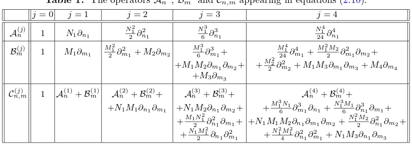
Table 1. The operatorsA(nj),Bm(j) andC(n,mj) appearing in equations (2.10).
hypothesis on the C(∞) property of the function u
n,m and on the radius of convergence of its
Taylor expansion for all shifts in the indices n andm involved in the difference equation (2.9), we can write a series representation of un+k,m+j around un,m. We choose the slow variables as
nk=. ǫnkn,mj
where the various constants Nk,Mj and ǫare all real numbers. In this presentation we assume
Kn= 1 and Km=K (eventually K= +∞) so that
sions (2.10) of the shift operators into equation (2.9), this turns into a PDE of infinite order. So we will assume for the function un,m =u(n, m, n1,{mj}Kj=1, ǫ) a double expansion in harmonics
and in the perturbative parameter ǫ
un,m=
in order to ensure the reality of un,m. The index γ is chosen ≥1 so that the nonlinear terms
of equation (2.9) enter as a perturbation in the multiple scale expansion. For simplicity we will setN1 =Mj = 1,j ≥1. Moreover we will assume that the functionsu(
θ)
γ satisfy the asymptotic
conditions lim
n1→±∞
u(γθ)= 0, ∀γ and θ to provide a meaningful expansion.
2.1.2 From derivatives to shifts
We can rewrite the so obtained partial differential equation as a partial difference equa-tion inverting the expansion of the partial shift operator in term of partial derivatives (2.8). From (2.8) we have
∂n1 = 1
ǫlnT
(ǫ)
n1 = 1
ǫln 1 +ǫ∆
(+)
n1 .
=
+∞
X
k=1
(−ǫ)k−1
k
∆(+)n1 k
, (2.12)
where ∆(+)n1
.
= (Tn(1ǫ) −1)/ǫ is the first forward difference operator with respect to the slow-variablen1. This is just one of the possible inversion formulae for the operatorTn(1ǫ). For example an expression similar to equation (2.12) can be written for the firstbackward difference operator ∆(n−1)
.
= 1−
Tn(1ǫ) −1
/ǫ. For the firstsymmetricdifference operator ∆(ns1)
.
= Tn(1ǫ)−
Tn(1ǫ) −1
/2ǫ
we get
∂n1 = sinh
−1ǫ∆(s)
n1
.
=
+∞
X
k=1
Pk−1(0)ǫk
k
∆(ns1)k ,
where Pk(0) is thek-thLegendre polynomial evaluated at x= 0.
Only when we impose that the function un is a slow-varying function of order ℓ in the
variable n1, i.e. that ∆ℓn+11 un = 0, we can see that the ∂n1 operator, which is given by formal series containing in general infinite powers of the ∆n1, reduces to polynomial of order at mostℓ. In [17], choosing ℓ = 2 for the indexes n1 and m1 and ℓ = 1 for m2, it was shown that the
integrablelattice potential KdV equation [20] reduces to a completely discrete and local nonlinear Schr¨odinger equation which has been proved to be not integrable by singularity confinement and algebraic entropy [13,23]. Consequently, if one passes from derivatives to shifts, one ends up in general with a nonlocal partial difference equation in the slow variables nκ and mδ.
2.2 The orders beyond the Schr¨odinger equation and the C-integrability conditions
The multiple scale expansion of an equation of the Burgers hierarchy on functions of infinite order will thus give rise to PDE’s. So a multiple scale integrability test will require that a dis-persive equation like equation (2.1) is C-integrable if its multiple scale expansion will go into the hierarchy of the Schr¨odinger equation
i∂tψ+∂x2ψ= 0.
To be able to verify the C-integrability we need to consider in principle all the orders beyond the Schr¨odinger equation. This in general will not be possible but already a few orders beyond the Schr¨odinger equation might be sufficient to verify if the equation is linearizable or not. In the case of S-integrable nonlinear PDE’s the first attempt to go beyond the NLSE order has been presented by Degasperis, Manakov and Santini in [8]. These authors, starting from an
S-integrable model, through a combination of an asymptotic functional analysis and spectral methods, succeeded in removing all the secular terms from the reduced equations order by order. Their results could be summarized as follows:
1. The number of slow-time variables required for the amplitudes u(jθ) appearing in (2.11) coincides with the number of nonvanishing coefficients of the Taylor expansion of the dispersion relation, ωj(κ) = j1!d
jω(k)
dkj .
2. The amplitudeu(1)1 evolves at the slow-times ms,s≥2 according to thes-th equation of
3. The amplitudes of the higher perturbations of the first harmonicu(1)j ,j≥2 evolve, taking into account some asymptotic boundary conditions, at the slow-timesms,s≥2 according
to certain linear, nonhomogeneous equations.
Then they concluded that the cancellation at each stage of the perturbation process of all the secular terms is a sufficient condition to uniquely fix the evolution equations followed by everyu(1)j ,j≥1 for each slow-timems. Point 2 implies that a hierarchy of integrable equations
provide for a function u always compatible evolutions, i.e. the equations in its hierarchy are generalized symmetriesof each other. In this way this procedure providesnecessary and sufficient conditions to get secularity-free reduced equations [8].
We apply the present procedure to the case of C-integrable partial difference equations. Following Degasperis and Procesi [9] we state the following theorem:
Theorem 1. If equation (2.9) is C-integrable then, after a multiple scale expansion, the func-tions u(1)j , j≥1 satisfy the equations
∂msu
(1)
1 −(−i)s
−1B
s∂ns1u
(1) 1
.
=Msu(1)1 = 0, (2.13a)
Msu(1)j =fs(j), (2.13b)
∀j, s≥2, where Bs∂ns1u
(j)
1 is the s-th f low in the linear Schr¨odinger hierarchy and Bs are real
constants. All the other u(jκ),κ≥2 are expressed as differential monomials ofu(1)r , r≤j−1.
In equation (2.13b)fs(j) is a nonhomogeneousnonlinear forcing written in term of differential
monomials ofu(1)r ,r≤j. From Theorem1it follows that a nonlinear partial difference equation
is said to be C-integrable if its asymptotic multiple scale expansion is given by a uniform asymptotic series whose leading harmonic u(1) possesses an infinity of generalized symmetries
evolving at different times and given by commuting linear equations. Equations (2.13) are a necessary condition for C-integrability.
It is worthwhile to stress here the non completely obvious fact that, in contrast to the first order wave equation, ∂tu = ∂xu, all the symmetries of the Schr¨odinger equation commuting
with it are given by the equations (2.13a) and only by them. This implies that all the equations appearing in the multiple scale expansion for aC-integrable equation are uniquely defined.
It is obvious that the operatorsMs defined in equation (2.13a) commute among themselves.
However the compatibility of equations (2.13b) is not always guaranteed but is subject to some compatibility conditions among their r.h.s. terms fs(j). Once we fix the indexj ≥2 in the set
of equations (2.13b), this commutativity condition implies the compatibility conditions
Msfs′(j) =Ms′fs(j), ∀s, s′≥2, (2.14)
where, as fs(j) and fs′(j) are functions of the different perturbations u(1)r of the fundamental
harmonic up to degreej−1, the time derivatives∂ms,∂ms′ appearing respectively inMsandMs′ have to be eliminated using the evolution equations (2.13) up to the index j−1. These last commutativity conditions turn out to be a linearizability test.
Following [8] we conjecture that the relations (2.13) are a sufficient condition for the C -integrability or that theC-integrability is anecessary condition to have a multiple scale expan-sion where equations (2.13) are satisfied. To characterize the functions fs(j) we introduce the
following definitions:
Definition 1. A differential monomialM u(1)j
,j≥1 in the functionsu(1)j , its complex conju-gate and itsn1-derivatives is a monomial of “gauge” 1 if it possesses the transformation property
M
˜
u(1)j
=eiθM u(1)j
Definition 2. A finite dimensional vector spacePν,ν ≥2 is the set of all differential
polyno-mials of gauge 1 in the functions u(1)j , j≥1, their complex conjugates and theirn1-derivatives
such that their total order in ǫisν, i.e.
order ∂nµ1u(1)j
= order ∂nµ1u¯(1)j
=µ+j=ν, µ≥0.
Definition 3. Pν(µ), µ ≥ 1 and ν ≥ 2 is the subspace of Pν whose elements are differential
polynomials of gauge 1 in the functionsu(1)j , their complex conjugates and theirn1-derivatives
such that their total order is ν and 1≤j≤µ.
From Definition 3 it follows that Pν = Pν(ν−2). Moreover in general fs(j) ∈ Pj+s(j−1)
where j, s ≥ 2. The basis monomials of the spaces Pν(µ) in which we can express the
func-tionsfs(j) can be found, for example, in [25].
Proposition 1. If for each fixed j≥2 the equation (2.14) withs= 2 and s′ = 3, namely
M2f3(j) =M3f2(j), (2.15)
is satisfied, then there exist unique differential polynomials fs(j) ∀s ≥ 4 such that the flows
Msu(1)j =fs(j) commute for anys≥2 [24,6].
Hence among the relations (2.14) only those with s= 2 and s′ = 3 have to be tested.
Proposition 2. The homogeneous equation Msu= 0 has no solution u in the vector space Pµ,
i.e. Ker (Ms)∩ Pµ=∅.
Consequently the multiple scale expansion (2.13) is secularity-free. This does not mean that, in solving equation (2.13b), we have to set to zero all the contributions to the solution coming from the homogeneous equation but only that part of it which is present in the forcing terms. Finally:
Definition 4. If the relations (2.14) are satisfied up to the index j, j ≥ 2, we say that our equation is asymptotically C-integrable of degreej orAj C-integrable.
2.2.1 Integrability conditions for the Schr¨odinger hierarchy
Here we present the conditions for the asymptoticC-integrability of orderkorAkC-integrability
conditions with k= 1,2,3. To simplify the notation, we will use foru(1)j the concise formu(j). TheA1C-integrability condition is given by the absence of the coefficientρ2 of the nonlinear
term in the NLSE (1.1).
The A2 integrability conditions are obtained choosing j = 2 in the compatibility
condi-tions (2.14) with s = 2 and s′ = 3 as in (2.15). In this case we have that f2(2) ∈ P4(1)
and f3(2) ∈ P5(1) where P4(1) contains 2 different differential monomials and P5(1) contains
5 different differential monomials, so that f2(2) and f3(2) will be respectively identified by 2
and 5 complex constants
f2(2)=. au,n1(1)|u(1)|
2+bu¯
,n1(1)u(1)
2, (2.16)
f3(2)=. α|u(1)|4u(1) +β|u,n1(1)|
2u(1) +γu
,n1(1)
2u¯(1) +δu¯
,2n1(1)u(1)
2+ε|u(1)|2u
,2n1(1).
In this way, eliminating from equation (2.15) the derivatives of u(1) with respect to the slow-times m2 and m3 using the evolutions (2.13a) with s = 2,3 and equating term by term, we
appearing in f2(2). The expression of the coefficientsα,β, γ,δ,ε appearing inf3(2) in terms
of aand bare
α= 0, β=−3iB3b
B2
, γ =−3iB3a 2B2
, δ= 0, ε=γ.
The A3 C-integrability conditions are derived in a similar way settingj = 3 in equation (2.15).
In this case we have that f2(3) ∈ P5(2) and f3(3) ∈ P6(2) where P5(2) contains 12 different
differential monomials and P6(2) contains 26 different differential monomials, so that f2(3)
and f3(3) will be respectively identified by 12 and 26 complex constants
f2(3)=. τ1|u(1)|4u(1) +τ2|u,n1(1)|
2u(1) +τ
3|u(1)|2u,2n1(1) +τ4u¯,2n1(1)u(1)
2
+τ5u,n1(1)
2u¯(1) +τ
6u,n1(2)|u(1)|
2+τ
7u¯,n1(2)u(1)
2+τ
8u(2)2u¯(1) (2.17)
+τ9|u(2)|2u(1) +τ10u(2)u,n1(1)¯u(1) +τ11u(2)¯u,n1(1)u(1) +τ12u¯(2)u,n1(1)u(1),
f3(3)=. γ1|u(1)|4u,n1(1) +γ2|u(1)|
2u(1)2u¯
,n1(1) +γ3|u(1)|
2u
,3n1(1) +γ4u(1)
2u¯
,3n1(1)
+γ5|u,n1(1)|
2u
,n1(1) +γ6u¯,2n1(1)u,n1(1)u(1) +γ7u,2n1(1)¯u,n1(1)u(1) +γ8u,2n1(1)u,n1(1)¯u(1) +γ9|u(1)|
4u(2) +γ
10|u(1)|2u(1)2u¯(2) +γ11u¯,n1(1)u(2)
2
+γ12u,n1(1)|u(2)|
2+γ
13|u,n1(1)|
2u(2) +γ
14|u(2)|2u(2) +γ15u,n1(1)
2u¯(2)
+γ16|u(1)|2u,2n1(2) +γ17u(1)
2u¯
,2n1(2) +γ18u(2)¯u,2n1(1)u(1) +γ19u(2)u,2n1(1)¯u(1) +γ20u¯(2)u,2n1(1)u(1) +γ21u(2)u,n1(2)¯u(1) +γ22u¯(2)u,n1(2)u(1) +γ23u,n1(2)u,n1(1)¯u(1) +γ24u,n1(2)¯u,n1(1)u(1) +γ25u¯,n1(2)u,n1(1)u(1) +γ26u¯,n1(2)u(2)u(1).
Let us eliminate from equation (2.15) withj= 3 the derivatives ofu(1) with respect to the slow-times m2 and m3 using the evolutions (2.13a) with s = 2,3 and the same derivatives of u(2)
using the evolutions (2.13b) withs= 2,3. Equating the remaining terms term by term, theA3
C-integrability conditions turn out to be:
τ1 =−
i
4B2
[b(τ11−2τ6) + ¯aτ7], ¯bτ7 =
1
2(b−a) (τ11+τ10−τ6) + ¯aτ7,
aτ8 =bτ8 = 0, aτ9 =bτ9 = 0, ¯aτ12=a(τ10−τ11) +bτ6+ ¯aτ7,
¯b−¯a
τ12= (b−a)τ10. (2.18)
Sometimesaandbturn out to be both real. In this case the conditions given in equations (2.18) becomes:
R1=
1 4B2
[b(I11−2I6) +aI7], I1 =−
1 4B2
[b(R11−2R6) +aR7],
(b−a) (R11+R10−R6−2R7) = 0, (b−a) (I11+I10−I6−2I7) = 0,
(b−a)R8= 0, (b−a)I8 = 0, (b−a)R9= 0, (b−a)I9 = 0,
a(R12+R11−R10−R7) =bR6, a(I12+I11−I10−I7) =bI6,
(b−a) (R12−R10) = 0, (b−a) (I12−I10) = 0, (2.19)
where τi=Ri+iIi for i= 1, . . . ,12. The expressions of theγj as functions of theτi are:
γ1=
3B3
4B22 aτ6−4iB2τ1+ ¯bτ12
, γ2=
3B3
4B22(bτ6+ ¯aτ7),
γ3=−
3iB3τ3
2B2
, γ4 = 0, γ5 =−
3iB3τ2
2B2
, γ6 =−
3iB3τ4
B2
γ7=γ5, γ8=γ3−3iB3τ5
B2
, γ9=γ10=γ11= 0,
γ12=−3iB3τ9
2B2
, γ13=−3iB3τ11
2B2
, γ14= 0, γ15=−3iB3τ12
2B2
,
γ16=−
3iB3τ6
2B2
, γ17=γ18= 0, γ19=−
3iB3τ10
2B2
, γ20=γ15,
γ21=−
3iB3τ8
B2
, γ22=γ12, γ23=γ16+γ19, γ24=γ13,
γ25=−
3iB3τ7
B2
, γ26= 0.
The conditions given in equations (2.18), (2.19) appear to be new. Their importance resides in the fact that a C-integrable equation must satisfy those conditions.
3
Linearizability of the equations of the Burgers hierarchy
Taking into account the results of the previous section we can carry out the multiple scale expansion of the equations of the Burgers hierarchy. To do so we substitute the definition (2.11) into equations (2.1), (2.6) and write down the coefficients of the various harmonicsθand of the various orders j of ǫ. When we deal with the differential-difference equation (2.1), we have to make the substitutions σm → t, σmi → ti. This transformation implies that in this case the
corresponding coefficientsρ2 andB2 will turn out to beσ-independent. In Appendix we present
all relevant equations and here we just present their results.
Proposition 3. The differential-difference equation (2.1) of the Burgers hierarchy satisfies the A1 (and consequently also the A2) and also the A3 C-integrability conditions.
Proposition 4. The partial difference Burgers-like equation (2.6) reduces for j= 3 and α= 1 to a NLSE with a nonlinear complex coefficient ρ2 given by equation (A.9c). Thus the equation
is neither S-integrable norC-integrable.
4
Conclusions
In the present paper we have presented all the steps necessary to apply the perturbative multiple scale expansion to dispersive nonlinear differential-difference or partial difference equations which may be linearizable. These passages involve the representation of the lattice variables in terms of an infinite set of derivative with respect to the lattice index and the analysis of the higher order of the perturbation which give rise to a set of compatible higher order linear PDE’s belonging to the hierarchy of the Schr¨odinger equation. The compatibility of these equations give rise to a linearizability test. We applied the so obtained test to the case of a differential-difference dispersive Burgers equation and its discretization. It turns out that the Burgers is linearizable (as it should be) but its discretization is neither S-integrable nor C-integrable. So, effectively this procedure is able to distinguish between linearizable and non-linearizable equations.
A
Appendix
Let us now start performing a multiple scale analysis of the partial difference equation (2.6). We present here the equations we get at the various orders of ǫand for the different harmonicsθ.
• Order ǫ and θ= 1: If one requires that u(1)1 6= 0, one obtains the dispersion relation
which implies that u(1)1 has the form
u(1)1 =g(ξ, mj, j≥2) exp
hence it is a secular term. As a consequence we have to require that
∂m1u
Solving equation (A) taking into account equation (A.4), we obtain
u(0)2 =f(ρ, mj, j≥2)−hδcos (ωσ)
arbitrary value of the variableξ. Let us restrict ourselves for simplicity to the case where there is no dependence at all on ρ. If one wants that the harmonic u(0)1 depends onξ and not on ρ, from equation (A.2) one has that ∂ξu(0)1 = 0, so that u(0)1 depends on the slow
variables mj,j ≥2 only. Similarly we have that ∂ξf = 0. In this case, in order to satisfy
the asymptotic conditions lim
ξ→±∞u
(0)
γ = 0, γ = 1, 2, one has to take u(0)1 =f = 0 (unless
we take the fully continuous limit h → 0, hn1 =. x1, σ → 0, σm1 =. t1 in which ρ → ξ).
Equation (A.7) then becomes
• Order ǫ3 and θ = 1: Taking into account the dispersion relation (A.1) and the equa-tionsu(0)1 = 0, (A.3), (A.5), (A.8), we have
∂m1u
(1) 2 −
σcos (κh)
hcos (ωσ)∂n1u
(1)
2 =−∂m2u
(1)
1 −iB2∂ξ2u
(1) 1 −iρ2
u(1)1
2
u(1)1 , (A.9a)
B2 =.
hσ h2−σ2
sin (κh) 2
σ2sin2(κh)−h2
cos (ωσ), (A.9b)
ρ2=. −
2hσsin2(ωσ/2) [2 cos (κh/2)−cos (3κh/2)] sin (κh/2) [cos (κh)−cos (ωσ)] cos (ωσ)
−2ihσsin
2(ωσ/2) sin (κh/2) sin (κh/2)
[cos (κh)−cos (ωσ)] cos (ωσ) . (A.9c)
As a consequence of equation (A.3) with u(0)1 = 0, the right hand side of equation (A.9a) is secular. Hence we have to require that
∂m1u
(1) 2 −
σcos (κh)
hcos (ωσ)∂n1u
(1)
2 = 0, (A.10a)
i∂m2u
(1)
1 =B2∂ξ2u
(1) 1 +ρ2
u
(1) 1
2
u(1)1 . (A.10b)
Equation (A.10a) implies thatu(1)2 also depends onξ while equation (A.10b) is a nonintegrable nonlinear Schr¨odinger equation, as from the definition (A.9c) we can see that ρ2 is a complex
coefficient. So we can conclude that equation (2.6) is notA1-integrable.
Let us perform the multiple scale reduction of the Burgers equation (2.1). Equation (2.1) can be always obtained as a semicontinuous limit of equation (2.6) defining the slow timestj =. σmj,
j≥1. In such a way we can use in the present calculation the results presented up above.
• Order ǫ and θ= 0: In this case the resulting equation is automatically satisfied.
• Order ǫ and θ = 1: Taking the semi continuous limit of equation (A.1), one obtains the dispersion relation
ω=−sin (κh)
h . (A.11)
• Order ǫ2 and θ= 0: Taking the semi continuous limit of equation (A.2), one obtains
∂t1u
(0) 1 −
1
h∂n1u
(0)
1 = 0, (A.12)
which implies that u(0)1 depends on the variableρ=. hn1+t1.
• Order ǫ2 and α= 1: Taking the semi continuous limit of equation (A.3), one obtains
∂t1u
(1) 1 −
cos (κh)
h ∂n1u
(1)
1 + 2 sin2(κh/2)u (0) 1 u
(1)
1 = 0, (A.13)
which implies that u(1)1 has the form
u(1)1 =g(1)(ξ, tj, j ≥2) exp
−
Z ρ
ρ0
u(0)1 ρ′ dρ′
, (A.14)
whereξ =. hn1+ cos (κh)t1,g(1) is an arbitrary function of its arguments going to zero as
• Order ǫ2 and θ= 2: Taking the semi continuous limit of equation (A.5), one obtains
u(2)2 = h 1−eiκhu
(1)2
1 . (A.15)
• Order ǫ3 and θ= 0: Taking the semi continuous limit of equation (A.6), one obtains
∂t1u
1 is a solution of the left hand side of equation (A.16),
hence it is a secular term. As a consequence we have to require that
∂t1u
Solving equation (A.17) taking into account equation (A.14), we obtain
u(0)2 =f(ρ, tj, j ≥2) +h
wheref is an arbitrary function of its arguments going to zeroρ→ ±∞.
• Order ǫ3 and θ= 1: For simplicity, from now on we require no dependence onρ1 so that, in order to satisfy the asymptotic conditions, it necessarily follows that
u(0)1 =f = 0. (A.19)
Taking the semi continuous limit of equations (A.9a), (A.9b), one obtains
∂t1u is secular. Hence we have to require that
∂t1u
Equation (A.21a) implies thatu(1)2 depends also onξ while, contrary to equation (A.10b), equation (A.21b) now is a linear Schr¨odinger equation, reflecting the C-integrability of equation (2.1).
• Order ǫ3 and α = 2: Taking into account the dispersion relation (A.11), the fact that
u(0)1 = 0 and the equations (A.13), (A.15), we have
• Orderǫ3andθ= 3: Taking into account the dispersion relation (A.11) and equation (A.15),
Solving equation (A.24), we obtain
u(0)3 =τ(ρ, tj, j≥2) +h u(1)2 u(
where τ is an arbitrary function of its arguments going to zero as ρ → ±∞. As usually, if we don’t want any dependence at all from ρ but only on ξ, in order to satisfy the asymptotic conditions lim
ξ→±∞u
(0)
3 = 0, we have to take
τ = 0 (A.26)
(unless we take the fully continuous limit).
• Order ǫ4 and θ = 1: Taking into account the dispersion relation (A.11) and equations (A.15), (A.18), (A.19), (A.22), (A.25), (A.26), we get equation (A.27) is secular, so that
∂t1u
The first relation implies thatu(1)3 also depends onξwhile the second one, as a consequence of equation (A.21b), implies that the right hand side is secular, so that
i∂t2u
• Order ǫ4 and θ = 2: Taking into account the dispersion relation (A.11) and the
• Order ǫ4 and θ = 3: Taking into account the dispersion relation (A.11) and the
equa-• Order ǫ4 and θ = 4: Taking into account the dispersion relation (A.11) and the
equa-tions (A.15), (A.23), we get
Solving equation (A.31), we obtain
u(0)4 = Θ (ρ, tj, j ≥2) +h u(1)1 u
where Θ is an arbitrary function of its arguments going to zero as ρ→ ±∞. As usually, if we don’t want any dependence fromρ but only on ξ, in order to satisfy the asymptotic conditions lim
ξ→±∞u
(0)
4 = 0, we have to take
Θ = 0
(unless we take the fully continuous limit).
• Order ǫ5 and θ = 1: Taking into account the dispersion relation (A.11) and equations
u(0)1 =f =τ = Θ = 0, together with the equations (A.15), (A.18), (A.22), (A.23), (A.25), side of equation (A.33) is secular, so that
∂t2u
(1)
3 +iB2∂2ξu
(1)
3 =−∂t4u
(1) 1 −∂t3u
(1)
2 −B3∂ξ3u
(1) 2
+iB4∂ξ4u
(1) 1 +ζ
h u(1)1
∂n1u
(1) 1
2
+u(1−1) ∂n1u
(1) 1
2
+u(1)21 ∂n21u(1−1)i. (A.34)
The first relation tells us that u(1)4 depends on ξ too while in the second one, as a con-sequence of equations (A.21b), (A.29a), the first our terms in the right hand side of equation (A.34) are secular, so that
∂t2u
(1)
3 +iB2∂2ξu
(1) 3 =ζ
h u(1)1
∂n1u
(1) 1
2
+u(1−1) ∂n1u
(1) 1
2
+u(1)21 ∂n21u(1−1)i, (A.35a)
∂t3u
(1)
2 +B3∂ξ3u
(1)
2 =−∂t4u
(1)
1 +iB4∂ξ4u
(1)
1 . (A.35b)
As a consequence of equation (A.29b), the right hand side of equation (A.35b) is secular so that
∂t3u
(1)
2 +B3∂ξ3u
(1)
2 = 0, ∂t4u
(1)
1 −iB4∂ξ4u
(1) 1 = 0.
Equation (A.35a), as one can see from the definition (2.17) and taking into account that a = b = 0, has a forcing term f2(3) that respects all the A3 C-integrability
con-ditions (2.18).
Acknowledgements
The authors have been partly supported by the Italian Ministry of Education and Research, PRIN “Nonlinear waves: integrable finite dimensional reductions and discretizations” from 2007 to 2009 and PRIN “Continuous and discrete nonlinear integrable evolutions: from water waves to symplectic maps” from 2010.
References
[1] Agrotis M., Lafortune S., Kevrekidis P.G., On a discrete version of the Korteweg–de Vries equation,Discrete Contin. Dyn. Syst.(2005), suppl., 22–29.
[2] Burgers J.M., A mathematical model illustrating the theory of turbulence, Adv. Appl. Mech. 1 (1948),
171–199.
[3] Calogero F., Why are certain nonlinear PDEs both widely applicable and integrable?, in What is Integra-bility?, Editor V.E. Zakharov,Springer Ser. Nonlinear Dynam., Springer, Berlin, 1991, 1–62.
[4] Calogero F., Eckhaus W., Necessary conditions for integrability of nonlinear PDEs, Inverse Problems 3
(1987), L27–L32.
Calogero F., Eckhaus W., Nonlinear evolution equations, rescalings, model PDEs and their integrability. I,
Inverse Problems3(1987), 229–262.
Calogero F., Eckhaus W., Nonlinear evolution equations, rescalings, model PDEs and their integrability. II,
Inverse Problems4(1987), 11–33.
Calogero F., Degasperis A., Ji X-D., Nonlinear Schr¨odinger-type equations from multiple scale reduction of PDEs. I. Systematic derivation,J. Math. Phys.41(2000), 6399–6443.
Calogero F., Degasperis A., Ji X-D., Nonlinear Schr¨odinger-type equations from multiple scale reduction of PDEs. II. Necessary conditions of integrability for real PDEs,J. Math. Phys.42(2001), 2635–2652.
Calogero F., Maccari A., Equations of nonlinear Schr¨odinger type in 1 + 1 and 2 + 1 dimensions obtained from integrable PDEs, in Inverse Problems: an Interdisciplinary Study (Montpellier, 1986),Adv. Electron. Electron Phys., Suppl. 19, Editors C.P. Sabatier, Academic Press, London, 1987, 463–480.
[5] Cole J.D., On a quasi-linear parabolic equation occurring in aerodynamics, Quart. Appl. Math.9(1951),
225–236.
[6] Degasperis A., Private communication.
[7] Degasperis A., Holm D.D., Hone A.N.I., A new integrable equation with peakon solutions,Teoret. Mat. Fiz.
[8] Degasperis A., Manakov S.V., Santini P.M., Multiple-scale perturbation beyond the nonlinear Schr¨odinger equation. I,Phys. D100(1997), 187–211.
[9] Degasperis A., Procesi M., Asymptotic integrability, in Symmetry and Perturbation Theory, SPT98 (Rome, 1998), Editors A. Degasperis and G. Gaeta, World Sci. Publ., River Edge, NJ, 1999, 23–37.
Degasperis A., Multiscale expansion and integrability of dispersive wave equations, in Integrability, Editor A.V. Mikhailov, Springer, Berlin, 2009, 215–244.
[10] Hernandez Heredero R., Levi D., Petrera M., Scimiterna C., Multiscale expansion of the lattice potential KdV equation on functions of an infinite slow-varyness order,J. Phys. A: Math. Theor. 40(2007), F831–
F840,arXiv:0706.1046.
[11] Hernandez Heredero R., Levi D., Petrera M., Scimiterna C., Multiscale expansion on the lattice and integra-bility of partial difference equations,J. Phys. A: Math. Theor.41(2008), 315208, 12 pages,arXiv:0710.5299.
[12] Hernandez Heredero R., Levi D., Petrera M., Scimiterna C., Multiscale expansion and integrability pro-perties of the lattice potential KdV equation, J. Nonlinear Math. Phys. 15 (2008), suppl. 3, 323–333,
arXiv:0709.3704.
[13] Hietarinta J., Viallet C., Singularity confinement and chaos in discrete systems,Phys. Rev. Lett.81(1998),
325–328,solv-int/9711014.
[14] Hopf E., The partial differential equationut+uux=uxx,Comm. Pure Appl. Math.3(1950), 201–230. [15] Kodama Y., Mikhailov A.V., Obstacles to asymptotic integrability, in Algebraic Aspects of Integrable
Sys-tems,Progr. Nonlinear Differential Equations Appl., Vol. 26, Birkh¨auser Boston, Boston, MA, 1997, 173–204. Hiraoka Y., Kodama Y., Normal form and solitons, in Integrability, Editor A.V. Mikhailov, Springer, Berlin, 2009, 175–214,nlin.SI/0206021.
[16] Leon J., Manna M., Multiscale analysis of discrete nonlinear evolution equations, J. Phys. A: Math. Gen. 32(1999), 2845–2869,solv-int/9902005.
[17] Levi D., Multiple-scale analysis of discrete nonlinear partial difference equations: the reduction of the lattice potential KdV,J. Phys. A: Math. Gen.38(2005), 7677–7689,nlin.SI/0505061.
[18] Levi D., Hernandez Heredero R., Multiscale analysis of discrete nonlinear evolution equations: the reduction of the dNLS,J. Nonlinear Math. Phys.12(2005), suppl. 1, 440–448.
[19] Levi D., Petrera M., Discrete reductive perturbation technique,J. Math. Phys.47(2006), 043509, 20 pages,
math-ph/0510084.
[20] Levi D., Petrera M., Continuous symmetries of the lattice potential KdV equation,J. Phys. A: Math. Theor. 40(2007), 4141–4159,math-ph/0701079.
[21] Levi D., Ragnisco O., Bruschi M., Continuous and discrete matrix Burgers’ hierarchies, Nuovo Ci-mento B (11)74(1983), 33–51.
[22] Levi D., Scimiterna C., The Kundu–Eckhaus equation and its discretizations,J. Phys. A: Math. Theor.42
(2009), 465203, 8 pages,arXiv:0904.4844.
[23] Ramani A., Grammaticos B., Tamizhmani K.M., Painlev´e analysis and singularity confinement: the ultimate conjecture,J. Phys. A: Math. Gen.26(1993), L53–L58.
[24] Santini P.M., The multiscale expansions of difference equations in the small lattice spacing regime, and a vicinity and integrability test. I,J. Phys. A: Math. Theor.43(2010), 045209, 27 pages,arXiv:0908.1492.
[25] Scimiterna C., Multiscale techniques for nonlinear difference equations, Ph.D. Thesis, Roma Tre University, 2009.
[26] Schoombie S.W., A discrete multiscales analysis of a discrete version of the Korteweg–de Vries equation,
J. Comp. Phys.101(1992), 55–70.