getdoc8d6a. 381KB Jun 04 2011 12:04:39 AM

El e c t ro n ic

Jo ur

n a l o

f P

r o

b a b i_{l i t y}

Vol. 13 (2008), Paper no. 53, pages 1479–1526. Journal URL

http://www.math.washington.edu/~ejpecp/

Large Deviations for One Dimensional Diffusions

with a Strong Drift

Jochen Voss

∗

(

Jochen.Voss@warwick.ac.uk

₎

Abstract

We derive a large deviation principle which describes the behaviour of a diffusion process with additive noise under the influence of a strong drift. Our main result is a large deviation theorem for the distribution of the end-point of a one-dimensional diffusion with drift ϑb where b is a drift function andϑa real number, whenϑconverges to∞. It transpires that the problem is governed by a rate function which consists of two parts: one contribution comes from the Freidlin-Wentzell theorem whereas a second term reflects the cost for a Brownian motion to stay near a equilibrium point of the drift over long periods of time.

Key words: large deviations, diffusion processes, stochastic differential equations. AMS 2000 Subject Classification:Primary 60F10,60H10.

Submitted to EJP on April 28, 2005, final version accepted November 15, 2006.

1

Introduction

The Freidlin-Wentzell theorem and its generalisations are well-known large deviation results. This theorem provides a large deviation principle (LDP) on the path space for solutions of the SDEd X =

b(X)d t+pǫd Bwhenǫconverges to 0. The related, but different, problem of the large deviation behaviour of a diffusion process under the influence of a strong drift is less studied. In this article we derive an LDP for the behaviour of the endpoint Xϑ_t of solutions of the R_{-valued stochastic}

differential equation

d X_sϑ=ϑb(X_sϑ)ds+d B_s for alls_∈[0,t]

X₀ϑ=z_∈R (1.1)

when the parameterϑconverges to infinity.

For comparison with the Freidlin-Wentzell result one can convert the case of strong drift into the case of weak noise with the help of the following scaling argument: Define ˜X_sϑ=X_sϑ_/ϑ and ˜B_s=pϑB_s/ϑ

for alls_∈[0,ϑt]. Then the process ˜Xϑ is a solution of the SDE

dX˜_sϑ=b(X˜_sϑ)ds+_p1

ϑd Bs for alls∈[0,ϑt] ˜

X₀ϑ=z

and we have

P(Xϑ_{t ∈}A) =P X˜ϑ_{∈ {}ω|ωϑt∈A}

.

The rescaled problem looks more similar to the situation from the Freidlin-Wentzell theory, but now the event in question depends on the parameterϑ. Thus the Freidlin-Wentzell theorem still does not apply easily. Therefore a more sophisticated proof will be required.

The text is structured as follows: In section 2 we state our main result and two corollaries. Since the proof of the theorem is quite long we give an overview of the proof of our theorem in section 3. The proof itself is spread over sections 4, 5 and 6.

The result presented in this text was originally derived as part of my PhD-thesis[Vos04].

2

Results

Recall that a family(Xϑ)_ϑ>0 of random variables with values in some topological space_X satisfies the LDP with rate functionI:_{X →}[0,_∞], if it satisfies the estimates

lim inf

ϑ→∞ 1

ϑlogP(X

ϑ

∈O)_{≥ −}inf

x∈OI(x)

for every open setO⊆ X and

lim sup

ϑ→∞ 1

ϑlogP(X

ϑ

∈A)_{≤ −}inf

x∈AI(x)

for every closed setA_{⊆ X}. The family(Xϑ)_ϑ>0 satisfies the weak LDP if the upper bound holds for every compact (instead of closed) set A⊆ X. For details about the theory of large deviations we refer to[DZ98].

Theorem 1. Let b:R_→R _{be a globally Lipschitz C}2_{-function with lim inf}

|x|→∞|b(x)|> 0. Assume

that there is an m∈R_{with b}(x) =0if and only if x=m and with b′(m)₆=0. Furthermore let z∈R_, t>0and for everyϑ >0let Xϑ be the solution of the SDE

d X_sϑ=ϑb(X_sϑ)ds+d Bs for s∈[0,t], and

X₀ϑ=z. (2.1)

Then the family(Xϑ_t)_ϑ>0satisfies the weak LDP onR_{with rate function}

J_t(x) =V_zm(Φ)₋Φ(z) +t(Φ′′(m))−+V_mx(Φ) + Φ(x) (2.2)

for all x _∈ R_{, where Φ satisfies b = −Φ}′_{, V}b

a(Φ) is the total variation ofΦ between a and b, and (Φ′′(m))− denotes the negative part of Φ′′(m), i.e. (Φ′′(m))− = 0 if Φ′′(m) _≥ 0 and (Φ′′(m))− = |Φ′′(m)_|ifΦ′′(m)<0.

Note that the condition b=₋Φ′ definesΦonly up to a constant, but the rate functionJ_t does not depend on the choice of this constant.

In the theorem V_ab(Φ) can be interpreted as the “cost” for the process of going froma to b. Using

b=₋Φ′we find

V_ab(Φ) =¯¯ Z b

a

|b(x)_|d x¯¯

for anya,b∈R_{. The term}(Φ′′(m))−can be interpreted as the “cost” of staying nearmfor a unit of time. This term only occurs, if the equilibrium pointmis unstable.

Given the sign of b′(m) the rate function from the theorem can be simplified because the drift b

has only one zero. The following corollary describes the case of b′(m)<0, which corresponds to attracting drift. In this case the weak LDP from the theorem can be strengthend to the full LDP.

Corollary 2. Under the conditions of theorem 1 with b′(m)<0the following claims hold.

a) For every t>0the family(X_tϑ)ϑ>0 satisfies the weak LDP onRwith rate function

J_t(x) =2 Φ(x)₋Φ(m)

for all x_∈R_{. (2.3)}

b) If b is monotonically decreasing, then the family(Xϑ_t)_ϑ>0satisfies the full LDP with rate function J_t.

In the situation of corollary 2 the rate function is independent of the interval length t and of the initial pointz. This makes sense, because for strong drift we would expect the process to reach the equilibrium very quickly. Because we have lim inf_|x|→∞|b(x)_|>0 the potentialΦconverges to+_∞

for|x| → ∞andJt is a good rate function. In fact the rate function coincides with the rate function

of the LDP for the stationary distribution as given in theorem 3 (This is an easy application of the Laplace principle, see e.g.[Vos04]for details).

Theorem 3. LetΦ:Rd _→R _{be differentiable and such thatexp}(₋2Φ(x))is a probability density on Rd_{. LetΦbe bounded from below withΦ∗=inf{Φ(x)| x ∈}Rd_{}>−∞. Finally let b=−gradΦbe} Lipschitz continuous.

Then for everyϑ≥1the stochastic differential equation

has a stationary distributionµϑand for every measurable set A⊆Rd we have

lim

ϑ→∞ 1

ϑlogµϑ(A) =−ess infx∈A2 Φ(x)−Φ∗

.

Proof. (of corollary 2) a) Since we assume thatmis the only zero of the drift b, for b′(m)<0 the pointmis the minimum ofΦ. In this case we haveV_zm(Φ) = Φ(z)₋Φ(m), V_mx(Φ) = Φ(x)₋Φ(m)

andΦ′′(m)>0, so the rate function simplifies to the expression given in formula (2.3).

b) To strengthen the weak LDP to the full LDP we have to check exponential tightness, i.e. we have to show that for everyc>0 there is ana>0 with

lim sup

ϑ→∞ 1

ϑlogP |X

ϑ

t −m|>a

<−c

(for reference see lemma 1.2.18 from [DZ98]). We use a comparison argument to obtain this estimate.

Using the assumption lim inf_|x|→∞|b(x)| >0 we find that exp(−2ϑΦ)is integrable and SDE (2.1) has a stationary distribution with density proportional to exp(₋2ϑΦ). LetXϑ be a solution of (2.1) with start in z and Yϑ be a stationary solution, both with respect to the same Brownian motion. Then we get the deterministic differential equation

d d t(X

ϑ

t −Y

ϑ

t ) =ϑ b(X

ϑ

t)−b(Y

ϑ

t )

for the difference between the processes. First assumeX₀ϑ₋Y₀ϑ _≥0. Because for X_tϑ₋Y_tϑ =0 the right hand side vanishes, the processX_tϑ−Y_tϑcan never change its sign and stays positive. Since b

is decreasing we haveb(X_tϑ)₋b(Y_tϑ)_≤0 and we can conclude 0_≤Xϑ_{t −}Y_tϑ_≤X₀ϑ₋Y₀ϑ.

For the caseX₀ϑ₋Y₀ϑ_≤0 we can interchange the roles ofX andY to obtain the estimate 0≤Y_tϑ−Xϑ_t ≤Y₀ϑ−X₀ϑ.

Combining these two cases gives

|Y_tϑ₋X_tϑ_{| ≤ |}Y₀ϑ₋X₀ϑ_|=_|Y₀ϑ₋z_|.

Using

|Xϑ_t −m| ≤ |X_tϑ−Y_tϑ|+_|Y_tϑ−m| ≤ |z−Y₀ϑ|+_|Y_tϑ−m|

≤ |z−m|+_|Y₀ϑ−m|+_|Y_tϑ−m|

we can conclude

P |Xϑ_t −m|>a

≤P |Y₀ϑ−m|+_|Y_tϑ−m|>a− |z−m|

≤P_|Y₀ϑ₋m_|> a− |z−m| 2

+P_|Y_tϑ₋m_|> a− |z−m| 2

=2P_|Y₀ϑ₋m_|> a− |z−m| 2

Now letc>0. Then using theorem 3 we can find ana>0 with

lim

ϑ→∞ 1 ϑlogP

|Y₀ϑ₋m_|> a− |z−m| 2

≤ −c

and using the above estimate we get

lim

ϑ→∞ 1

ϑlogP |X

ϑ

t −m|>a

≤ −c.

Since this is the required exponential tightness condition, the proof is complete.

The case of repelling drift, i.e. of b′(m)>0, is described in the following corollary.

Corollary 4. Under the conditions of theorem 1 with b′(m)>0, for every t >0the family(Xϑ_t)_ϑ>0

satisfies the weak LDP onR_{with constant rate function}

Jt(x) =2 Φ(m)−Φ(z)

−tΦ′′(m). (2.4)

Proof. (of corollary 4) In the case b′(m) > 0 the point m is the maximum of Φ and because of

V_zm(Φ) = Φ(m)₋Φ(z),V_mx(Φ) = Φ(m)₋Φ(x)andΦ′′(m)<0 we get

J_t(x) = Φ(m)₋Φ(z)

−Φ(z)₋tΦ′′(m) + Φ(m)₋Φ(x)

+ Φ(x)

=2 Φ(m)₋Φ(z)

−tΦ′′(m)

for allx ∈R.

The corollary shows that in the case of repelling drift the rate function does not depend on x. In particular it is not a good rate function. Here it is impossible to strengthen the weak LDP to the full LDP because we have

lim

ϑ→∞ 1

ϑlogP(X

ϑ

t ∈R) =0 6= 2 Φ(m)−Φ(z)

−tΦ′′(m).

3

Overall Structure of the Proof

The remaining part of this text contains the proof of theorem 1. Since the proof is quite long, we use this section to give an overview of the proof. All the technical details are contained in sections 4, 5, and 6.

Let Xϑ be a solution of the SDE (1.1). From the Girsanov formula we know the density of the distribution ofXϑ_t w.r.t. the Wiener measureW_{: assumingX}ϑ

0 =0 andb=−∇Φwe get

P(X_tϑ_∈A) =

Z

1_A(ωt)exp ϑF(ω)−ϑ2G(ω)

dW_{(ω) (3.1)}

where

F(ω) = Φ(ω0)−Φ(ωt) +

1 2

Z t

0

Φ′′(ω_s)ds and

G(ω) = 1

2

Z t

0

For large values ofϑ theϑ2G term dominates over theϑF term and we show that the only paths which contribute for the large deviations behaviour ofX_tϑare those, which correspond to very small values of G. These paths run quickly to the equilibrium point mof the drift b, stay close to this point for most of the time, and shortly before time t move quickly into the setA. Assuming for the momentA=B(a,δ)with a smallδ >0, we get

P(Xϑ_t ≈a)_≈exp ϑ(Φ(0)₋Φ(a) + t

2Φ ′′_(m))

Z

1_{ωt≈a}exp −ϑ

2_G(ω)

dW(ω)

and thus

lim

ϑ→∞ 1

ϑlogP(X

ϑ

t ≈a)

≈Φ(0)₋Φ(a) + t

2Φ

′′_{(m) + lim}

ϑ→∞ 1 ϑlog

Z

1_{ω

t≈a}exp −

ϑ2

2

Z t

0

b2(ωs)ds

dW_(ω).

(3.2)

Lemma 26 in section 6 resolves the technical details which are hidden in the_≈-signs here and also gives the required upper and lower limits for (3.2).

To evaluate the integral on the right hand side of (3.2) we use the following result about upper and lower limits in Tauberian theorems of exponential type. The theorem is proved in[Vos04]. It is a generalisation of de Bruijn’s theorem (see theorem 4.12.9 in[BGT87]).

Theorem 5. Let X ≥ 0be a random variable and A an event with P(A) > 0. Define the upper and lower limits

¯

r =lim sup

λ→∞ 1

p

λlogE(e −λX₁

A) and r

¯=lim infλ→∞ 1

p

λlogE(e −λX₁

A)

as well as

¯

s=lim sup

ǫ→0

ǫlogP(X ≤ǫ,A) and s

¯=lim infǫ→0 ǫlogP(X ≤ǫ,A). Then₋¯r2/4=¯s and for the lower limits we have the sharp estimates₋r

¯ 2

≤s ¯≤ −¯r

2_/4.

Using theorem 5 we can reduce the original problem to the calculation of exponential rates like

lim

ǫ↓0ǫlogP Z t

0

b2(B_s)ds_≤ǫ,B_{t ≈}a.

In section 4 we examine the situation that during a short time interval the process runs from 0 tom

or frommtoarespectively while still keepingR b2(ωs)dssmall. This will be used for the initial and

the final section of the path. As indicated in section 1 we can rescale the problem in these domains and apply the known results for weak noise. The problem here is to identify the infimum of the rate function.

In section 5 we examine the situation thatR b2(ωs)ds is small over a long interval of time. This

will be used to study the middle section of the path. We will use theorem 5 again to deduce the probability for this case from the known Laplace transform ofRt

0B 2

s ds.

Finally, in section 6, we fit these two results together to complete the proof of theorem 1. This part of the proof is modelled after the proof of proposition 6 which we give below. We want to useX1,X2,X3=

R

the path respectively. Since these random variables are not independent, we cannot directly apply proposition 6 but have to use an enhanced version of the proof. This is provided in lemma 27.

We give the full prove of proposition 6 here, because we will need the proposition itself in the proof of lemma 23, and also because we hope that reading the proof of proposition 6 might make it easier to follow the proof of lemma 27 below.

Proposition 6. Let X₁, . . . ,X_nbe independent, positive random variables with

lim inf

ǫ↓0 ǫlogP Xk≤ǫ

=₋b2_k and lim sup

ǫ↓0

ǫlogP Xk≤ǫ

=₋c_k2

where b_k,c_k≥0for k=1, . . . ,n. Then we have

lim inf

ǫ↓0 ǫlogP X1+· · ·+Xn≤ǫ

≥ −(b₁+_{· · ·}+b_n)2

and

lim sup

ǫ↓0

ǫlogP X1+· · ·+Xn≤ǫ

≤ −(c1+· · ·+cn)2.

Proof. Letδ >0. Since the simplex

Sǫ_n=

(ǫ1, . . . ,ǫn)∈Rn_≥0 ¯

¯ǫ₁+· · ·+ǫ_n≤ǫ

is compact and covered by the open sets

(ǫ1, . . . ,ǫn) ∈ Rn

¯

¯ ǫ_j < α_jǫforj=1, . . . ,n for

α1, . . . ,αn>0 withα1+· · ·+αn=1+δ, we can find a finite set

Dδ_n ⊆

α∈Rn

>0 ¯

¯α₁+· · ·+α_n=1+δ (3.3)

with

S_nǫ⊆ [

α∈Dδ

n

(ǫ1, . . . ,ǫn)∈R_≥n0 ¯

¯ǫ_j≤α_jǫfor j=1, . . . ,n

for allǫ >0. This gives

P X₁+_{· · ·}+X_n≤ǫ

≤ X

α∈Dδ

n

P X_1≤α1ǫ, . . . ,Xk≤αkǫ

.

and for the individual terms in the sum we can use the relation

lim sup

ǫ↓0

ǫlogP X_1≤α1ǫ, . . . ,Xk≤αkǫ

=lim sup

ǫ↓0

ǫlog

n

Y

k=1

P Xk≤αkǫ

=₋

n

X

k=1 c_k2

αk

.

Let a=Pn_k=1αk, pk= αk/a, anddk= ck/pk fork=1, . . . ,n. Applying Jensen’s inequality to the

random variable which takes valuedk with probabilitypk gives

c₁2

α1

+_{· · ·}+ c

2

n

αn

≥(c1+· · ·+cn)

2

Pn k=1αk

where equality holds if and only if there is aλ∈R_{withλαk=ck fork=1, . . . ,n. Thus we get}

lim sup

ǫ↓0

ǫlogP X_1≤α1ǫ, . . . ,Xn≤αnǫ

≤ −(c1+· · ·+cn)

2

1+δ

for everyα∈Dδ_n. Using lemma 1.2.15 of[DZ98]we can conclude lim sup

ǫ↓0

ǫlogP X1+· · ·+Xn≤ǫ

≤max

α∈Dδ

n

lim sup

ǫ↓0

ǫlogP X1≤α1ǫ, . . . ,Xn≤αnǫ

≤ −(c1+· · ·+cn)

2

1+δ

for everyδ >0 and thus

lim sup

ǫ↓0

ǫlogP X₁+_{· · ·}+X_n≤ǫ

≤ −(c₁+_{· · ·}+c_n)2.

From (3.4) we know that we should chooseαkproportional tobkin order to get the optimal lower

bound. This leads to the estimate

lim inf

ǫ↓0 ǫlogP X1+· · ·+Xn≤ǫ

≥lim inf

ǫ↓0 ǫlogP Xk≤

bk

b1+· · ·+bn

ǫ,k=1, . . . ,n

=lim inf

ǫ↓0 ǫlog

n

Y

k=1

P Xk≤

b_k b₁+_{· · ·}+b_nǫ

≥ n

X

k=1

b₁+_{· · ·}+b_n

b_k lim infǫ↓0 ǫlogP Xk≤ǫ

=₋

n

X

k=1

b₁+_{· · ·}+b_n b_k b

2

k

=₋(b1+· · ·+bn)2

which completes the proof.

4

Reaching the Final Point

The results of this section help to estimate the probability that the path travels quickly between the equilibrium point of the drift and the final resp. initial point. Here Schilder’s theorem (see theorem 5.2.1 in[DZ98]) can be applied and we will reduce the evaluation of the rate function to a variational problem.

The main result of this section is the following proposition which describes the large deviation behaviour of the event

1 2

Z tǫ

0

whenǫ ↓0, where the final point B_tǫ stays in a fixed, compact set. Evaluating the rate for fixed

t>0 is difficult, but it transpires that there is an explicit representation for the limit of the rate ast

tends to infinity.

Proposition 7. Let Pz be the distribution of a Brownian motion with start in z and B be the canonical

process. Let b:R_→R _{be a C}2_{-function withlim inf|x|→∞|b(x)|>0. Assume that there is an m∈}R

The modulus of the integrals is taken to properly handle the cases m<z anda<m. The proof of proposition 7 is based on the following two lemmas. Lemma 8 evaluates the infimum of the rate function from Schilder’s theorem. Since the proof of lemma 8 is quite long, we defer the proof until the end of the section. We will writeC₀([0,t],R_{) =}

Consider the rate function

I_t(ω) =

(₁ 2

Rt 0|ω˙|

2_{ds, ifωis absolutely continuous, and}

Lemma 9. Let M_ta,z,β be as in lemma 8. Then for every pair K1,K2⊆Rof compact sets the set

M= [ z∈K1

[

a∈K2 [

0≤β≤1 M_ta,z,β

is closed in C₀([0,t],R_).

Proof. By definition of the setsM_ta,z,β we have

M = [ z∈K1

n

ω∈C[0,t]

¯ ¯

¯ω0=0,ωt+z∈K2,

1 2

Z t

0

v(ωr+z)d r≤1

o

.

Assume thatω∈C0([0,t],R)\M. Then eitherωt+z ∈/ K2 for all z∈K1, i.e.ωt lies outside the

compact setK₂₋K₁, or

1 2

Z t

0

v(ωr+z)d r>1

for everyz∈K2, i.e.

inf

z∈K2

1 2

Z t

0

v(ωr+z)d r >1

becauseK₂ is compact and v and the integral are continuous. In both cases we can find anǫ >0, such that the ballB(ω,ǫ)also lies inC₀([0,t],R_{)\M. ThusMis the complement of an open set.}

With these preparations in place we can now give the proof for proposition 7.

Proof. (of proposition 7) We want to apply Schilder’s theorem[DZ98, theorem 5.2.1]and to eval-uate the rate function using lemma 8. LetK₁,K_{2 ⊆}R_{be compact. Define the process ˜B by setting}

˜

Br= (Brǫ−z)/pǫfor everyr>0. Then ˜Bis a Brownian motion with start in 0 and we get

P_z1

2

Z tǫ

0

b2(B_s)ds_≤ǫ,B_tǫ∈K2

s=rǫ

= Pz

1

2

Z t

0

b2(Brǫ)d r≤1,Btǫ∈K2,

=P

1

2

Z t

0

b2(pǫ_B˜_r+z)d r≤1,pǫ_B˜_t+z∈K2

=PpǫB˜_∈ [

a∈K2 [

β≤1

M_ta,z,β

and thus

sup

z∈K1 Pz

Btǫ∈K2,

1 2

Z tǫ

0

b2(Bs)ds≤ǫ

≤P

p

ǫB˜∈ [ z∈K1

[

a∈K2 [

β≤1 M_ta,z,β

.

Since from lemma 9 we know that the set S_z∈K

t is closed in the path space

C0[0,t],k · k∞

, we can apply Schilder’s theorem to get

lim sup

for everyη >0. Together with the relation (4.2) this proves the upper bound.

For the lower bound we follow the same procedure. Without loss of generality we can assume that

Ois bounded. Here we get

is open in C₀[0,t],_{k · k∞}

. So we can use the lower bound from Schilder’s theorem and lemma 8 to complete the proof.

Corollary 10. Under the assumptions of proposition 7 we have

lim

η↓0lim inft→∞ lim infǫ↓0 ǫlogm−η≤infz≤m+ηPz

1

2

Z tǫ

0

b2(Bs)ds≤ǫ,Btǫ∈O

≥ −1₄ inf

a∈O

Z a

m

|b(x)_|d x 2

for every open set O⊆R_.

Proof. Forz∈R_define

M_tz=nω∈C[0,t]

¯ ¯

¯ω0=0,ωt+z∈O,

1 2

Z t

0

b2(ωs+z)ds<1

o

.

Let δ > 0. Choose an ˜ω ∈ M_tm with I_t(ω˜) < inf_{I_t(ω) _| ω ∈ M_tm_}+δ. Because O is open and b and the integral are continuous we can find an E > 0, such that for every η < E the ball

Bη(ω˜)⊆C0([0,t],R)is contained in all of the setsMtz form−η <z<m+η. This gives

lim inf

ǫ↓0 ǫlogm−η≤infz≤m+ηPz

1

2

Z tǫ

0

b2(Bs)ds≤ǫ,Btǫ∈O

=lim inf

ǫ↓0 ǫlogm−η≤infz≤m+ηPz

p

ǫB_∈M_tz

≥lim inf

ǫ↓0 ǫlogm−η≤infz≤m+ηPz

p

ǫB_∈B_η(ω˜).

and using Schilder’s theorem and the relation

−inf

I_t(ω)¯¯ω∈B_η(ω˜) ≥ −I_t(ω˜)>−inf

I_t(ω)¯¯ω∈Mm

t −δ

we find

lim inf

ǫ↓0 ǫlogm−η≤infz≤m+ηPz

1

2

Z tǫ

0

b2(B_s)ds_≤ǫ,B_tǫ∈O

≥ −inf

I_t(ω)¯¯ω∈B_η(ω˜)

>−inf

I_t(ω)¯¯ω∈Mm

t −δ.

Now we can evaluate the infimum on the right hand side as we did in proposition 7. We get

lim inf

t→∞ lim infǫ↓0 ǫlogm−η≤infz≤m+ηPz

1

2

Z tǫ

0

b2(B_s)ds_≤ǫ,B_tǫ∈O

≥ −1

4ainf∈O

Z a

m

|b(x)_|d x2₋δ

The only thing which remains to be done in this section is to give a proof for lemma 8. Before we do so we need some preparations. For the remaining part of this section we assume throughout that

vis non-negative and two times continuously differentiable and thata,z∈R_{are fixed.}

Notation: For x,y ∈R _{we will write}[x,y] for the closed interval between x and y; in the case

x < y this is to be read as[y,x]instead.

As a first step towards the proof of lemma 8 we get rid of the parameterβ.

Lemma 11. Let_{0_{} ⊂}B_⊆R

+be bounded. Assume that

lim

t→∞inf

I_t(ω)¯¯ω∈M_ta,z,1 =J(a,z)

locally uniform in a,z_∈R_{. Then the relation(4.1)holds.}

Proof. Letβ >0. Forω∈M_ta,z,β define ˜ωby

˜

ωr=ωrβ for allr∈[0,t/β].

Then we have ˜ω0=0, ˜ωt/β=ωt, and

1 2

Z t/β

0

v(ω˜r+z)d r s=rβ

= 1

β 1 2

Z t

0

v(ωs+z)ds.

Thusω7→ω˜ is a one-to-one mapping fromM_ta,z,β onto M_ta_/β,z,1. Because of

It/β(ω˜) =

1 2

Z t/β

0

˙ ˜

ω2_rd r= β

2

2

Z t/β

0

˙

ω2_rβd r s==rβ β

2

Z t

0

˙

ω2_s ds=βIt(ω)

we find

inf

I_t(ω)¯¯ω∈M

a,z,β

t =

1 βinf

I_t/β(ω)

¯

¯ω∈Ma,z,1

t/β .

Now letz_∈K₁ anda_∈K₂. Sincem∈/K_1∩K₂ every continuous pathωwithω0=0 andωt=a−z

has

1 2

Z t

0

v(ωs+z)ds>0,

the setM_ta,z,0is empty and we find

infnI_t(ω)

¯ ¯ ¯ω∈

[

β∈B

M_ta,z,βo= inf

β∈B\{0}inf

I_t(ω)¯¯ω∈Ma,z,

β

t

= inf

β∈B\{0} 1 βinf

I_t/β(ω)¯¯ω∈Ma,z,1

t/β .

Now letK1,K2⊆Rbe compact. Letη >0 and choose a t0>0 with

¯ ¯ ¯inf

I_t(ω)¯¯ω∈M_ta,z,1 −J(a,z) ¯ ¯

for allt>t₀,z_∈K₁, anda_∈K₂. Then for everyt>t₀supBand everyβ >0 we have

solve the Euler-Lagrange equations (see section 12 of[GF63]) for extremal values of I_t under the constraint

and with the boundary conditions

ω0=z and ωt=a.

Because of v ∈ C2(R) we can use theorem 1 from section 12.1 of [GF63] to find that for every extremal point ω of I, under the given constraints, there is a constant λ, such thatω solves the equations

Existence of solutions: the autonomous second order equation (4.3a) describes the motion of a classical particle on the real line in the potential₋λv. The differential equation can be reduced to an autonomous first order equation in the plane with the usual trick: defining x(s) = (ωs, ˙ωs)and

F(x₁,x₂) = x₂,λv′(x₁)

the equation becomes

˙

x(s) =F(x(s)) for alls∈[0,t].

See e.g. section 5.3 of[BR89]for details. Becausev′and thus F is locally Lipschitz continuous, for every pairω0=z, ˙ω0=v0of initial conditions and every bounded region we find a unique solution

There are two degrees of freedom in (4.3a) because we can choose ˙ω0 andλ. In the following we

will show, that the two additional conditions (4.3b) and (4.3c) guarantee the existence of a unique solution to the system (4.3).

Forλ=0 the only solution of (4.3a) and (4.3c) is given byω_s =z+ (a−z)s/t for 0≤s≤ t and consequently in this case we have

1 2

Z t

0

v(ωs)ds=th(z,a)

with

h(z,a) =

( ₁

2(a−z) Ra

z v(x)d x, if a6=z, and

1

2v(z) else.

Sincem₆= K_1∩K₂, z _∈K₁, anda _∈K₂ we have h(z,a)> 0 for everyz _∈K₁,a _∈K₂ and because

K_1×K₂ is compact we findc=inf_(z,a)∈K

1×K2h(z,a)>0. In the following assume t>1/c. Then we

know from (4.3b) that every solution of (4.3) hasλ6=0.

The interpretation as the motion of a classical particle helps us to determine the behaviour of the solutions. We can use conservation of energy: Because of

∂s

1 2ω˙

2

s −λv(ωs)

=ω˙sω¨s−λv′(ωs)ω˙s=ω˙s ω¨s−λv′(ωs)

(4.3a)

= 0

we have

1 2ω˙

2

s −λv(ωs) =

1 2ω˙

2

0−λv(ω0) =:E for alls∈[0,t]. (4.4)

This conservation law describes the speed for any point of the path: the speed of the path at pointωs

is

|ω˙s|=p2(E+λv(ωs)). (4.5)

Thus the rate functionIt can be expressed as a function of Eandλas follows.

I_t(ω) =1

2

Z t

0

˙ ω2_s ds=

Z t

0

E+λv(ωs)ds

=t E+2λ, (4.6)

whereλandEare determined by equations (4.3b) and (4.3c).

Because of relation (4.4) we find that wheneverωis a solution of (4.3a) we have E_{≥ −}λv(ωs)for

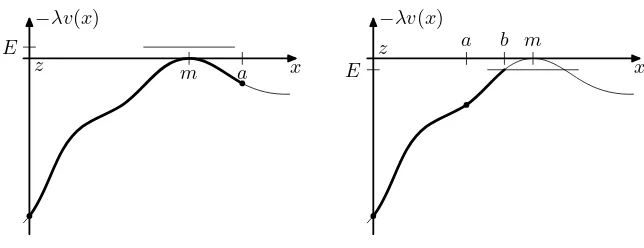
alls∈[0,t]and the path can only stop and turn at points x with₋λv(x) =E. Let x ∈R be such a point and assume v′(x) =0. Thenη with η_s = x for alls ≥ 0 is the unique solution of (4.3a) withη0 = x and ˙η0 = 0. Now assume thatωs = x for somes > 0. Then (ωs−r)r∈[0,s] is also a

solution of (4.3a) with start in x and initial speed 0, so we have ωs−r =ηr = x for all r ∈[0,s].

This shows that a point x 6=z withE=₋λv(x)and v′(x) =0 cannot be reached by a solutionω of (4.3a). Thus whenever a non-constant path reaches an x _∈R _{with E= −λv(x)then we have}

¨

ωs = λv′(ωs) 6=0 and the path always changes direction there. Figure 1 illustrates two different

kinds of solution, one whereωs moves monotonically and one where the path reaches a point b

x z

−λv(x)

E

m a x

z

−λv(x)

E

m

a b

Figure 1:This figure illustrates two types of solution for equation(4.3a). Here we only consider the case

λ >0. The curved line is the graph of the function x _{7→ −}λv(x). The bold part of the lines corresponds to the points visited by the path ω. The thick dots are ω0,−λv(ω0)

and ωt,−λv(ωt)

. Both solutions start at z∈K1, head towards a neighbourhood of the zero m, and finally reach a point a∈K2. The left hand image shows a free solution, i.e. one with E >0, the right hand image shows a bound solution, i.e. one with E_≤0where the pathωturns at the point b with₋λv(b) =E.

Since the differential equation (4.3a) is autonomous and since a solutionωchanges direction every time is reaches a pointx with₋λv(x) =E, the path can reach at most two distinct points of these nature. In this case the solution oscillates between these points periodically. Thus every solution of (4.3a) changes direction only a finite number of times before timet.

In order to find the path which minimises the rate functionI_t we need to keep track of the different possible traces of the path. For the remaining part of this section we use the following notation. The path(ωs)0≤s≤t is said to have traceT = (x0,x1, . . . ,xn)whenω0= x0,ωt = xn, and the path

ω moves monotonically in either direction from x_i−1 to x_i for i = 1, . . . ,n in order and changes direction only at the points x₁, . . . ,x_n−1. We use the abbreviation

|T|= n

X

i=1

|xi−xi−1|

for the length of the trace and sometimes identifyT with the setSn_i=1[x_i−1,x_i]of covered points to write minT, maxT, v|T, or inf_x∈T v(x). For positive functions f:R_→Rwe use the notation

Z

T

f(x)d x:= n

X

i=1 ¯ ¯

Z xi

xi−1

f(x)d x¯¯.

The absolute values are taken to make the integral positive even when xi < xi−1. If a solutionω

of (4.3a) has trace T = (x0,x1, . . . ,xn), this then implies that v(x1) = · · · = v(xn−1) = −E/λ

and each of the x₁, . . . ,x_n−1 is either minT or maxT. Between the points x_i the path is strictly monotonic, i.e. after the start inzit oscillates zero or more times between minT and maxT before it reachesaat time t. Using this notation we can formulate the following Lemma.

Lemma 12. Letλ,E∈R_{and a trace T} = (x0, . . . ,xn)be given. Then the following two conditions are

(j) The unique solutionω:[0,t]_→R_of

¨

ωs=λv′(ωs) for all s∈[0,t]

with initial conditionsω0 = z andω˙0 =sgn(x1−x0) p

2(E+λv(0))has trace T and solves(4.3b)

and(4.3c).

(ij) We have x0 = z, xn = a, E = −λv(xi) for i = 1, . . . ,n−1, as well as E > −λv(x) for all

minT <x <maxT , and the pair(λ,E)solves

Z

T

v(x)

p

E+λv(x)

d x=p8 (4.7a)

and

Z

T

1

p

E+λv(x)

d x=p2t. (4.7b)

Proof. Assume the conditions from(j). Thenωis a solution of (4.3a), there are timest0,t1, . . . ,tn

withωti = xi fori=0, . . . ,n, and between the times ti the process moves monotonically. For any

integrable, positive function g:R_→R_{substitution using (4.5) yields}

Z t

0

g(ωs)ds= n

X

i=1 Z ti

ti−1

g(ωs)ds

= n

X

i=1 Z xi

xi−1

g(x) d x

sgn(xi−xi−1) p

2(E+λv(x))

=

Z

T

g(x)

p

2(E+λv(x))

d x. (4.8)

Applying (4.8) to the functiong=vgives

1 (4.3b)= 1

2

Z t

0

v(ωs)ds

(4.8)

= _p1

8

Z

T

v(x)

p

E+λv(x)

d x.

This is equation (4.7a). Applying (4.8) to the constant functiong=1 gives

t=

Z t

0

1ds (4.8)= _p1

2

Z a

0

1

p

E+λv(x)

d x,

which is equation (4.7b).

Now assume condition (ij). Fori=1, . . . ,ndefine the functionFi by

F_i(x) = _p1

2

¯ ¯

Z x

xi−1

1

p

E+λv(x)

for all x between x_i−1 and x_i. Then F_i is finite because of (4.7b), strictly monotonic (increasing if

xi>xi−1and decreasing else), and has Fi(xi−1) =0. Further define

tk= k

X

i=1 Fi(xi).

Equation (4.7b) gives t_n = t. Because the functions F_i are monotonic they have inverse functions

F_i−1 and we can defineω:[0,t]_→R_by

ω(s) =F_i−1(s₋t_i−1) for alls_∈[t_i−1,t_i].

We will prove thatωsatisfies all the conditions from (j).

Because we have t_i−t_i−1 = F_i(x_i) and thus F_i−1(t_i−t_i−1) =x_i = F_i−₊1₁(t_i−t_i) the functionω is well-defined on the connection points at times t_i and is continuous. This also shows ωti = xi for i=0, 1, . . . ,nand especiallyω0= x0=zandωt=xn=a.

Because the F_i are differentiable at all points x strictly between x_i−1 and x_i, the function ω is differentiable on the intervals(t_i−1,t_i)with derivative

˙ ωs=

1

F_i′(ωs)

=sgn(xi−xi−1) p

2(E+λv(ωs)).

Becauseωis continuous and the limits lim_s→tiω˙sexist, we see thatωis even differentiable on[0,t]

with ˙ω0=sgn(x1−x0) p

2(E+λv(0))and ˙ωti =0 fori=1, . . . ,n−1.

Using the same kind of argument again, we find

¨ ωs=

sgn(x_i−x_i−1)

2p2(E−λv(ωs))

2λv′(ωs)sgn(xi−xi−1) p

2(E−λv(ωs)) =λv′(ωs),

first between the ti and then on the whole interval [0,t]. Thus ω really solves the differential

equation from (j).

Using the substitution

1 2

Z t

0

v(ωs)ds=

1

p

8

Z

T

v(x)

p

E+λv(x)

d x

as in the first part, we also get back (4.3b) from (4.7a).

Now we have reduced the problem of minimisingIt(ω)over the solutionsωof the system (4.3) to

the problem of minimising

I_t(E,λ) =t E+2λ

over the solutions(E,λ)of the system (4.7).

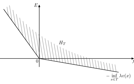
For a traceT define

H_T =

(E,λ)¯¯E≥ −inf

x∈Tλv(x) ⊆

R2

and furthermore define the functions f,g:H_t→[0,_∞]by

f(E,λ) =

Z

T

1

p

E+λv(x)

λ

0

E

−_xinf ∈T

λv₍x₎ HT

Figure 2: This figure illustrates the domain HT of the functions f and g. The domain is unbounded in

directionsλ → ∞and E _{→ ∞}. It is bounded from below by λ7→ −inf_x∈Tλv(x), which is equal to

−λsup_x∈T v(x)forλ≤0and to₋λinf_x∈Tv(x)forλ≥0.

and

g(E,λ) =

Z

T

v(x)

p

E+λv(x)

d x.

Figure 2 illustrates the domainH_T. Both functions are finite in the interior of the domain, but can be infinite at the boundary. The equations (4.7) are equivalent to f(Eλ,λ) =

p

2tandg(E,λ) =p8. For paths which change direction at some point we will find solutions(E,λ)of (4.7), which lay on the boundary of H_T. For paths which go straight from z to a we will find solutions (E,λ) in the interior ofHT.

Lemma 13. Let t>0and T be a trace from z_∈R_{to a∈}R_{such that v|T is not constant. Then there} is at most one solution(E,λ)of (4.7).

Proof. ForE>−inf_x∈Tλv(x)we can choose anE_∗between₋inf_x∈Tλv(x)andE. Thenv(x)/(E_∗+

λv(x))3/2is an integrable upper bound ofv(x)/(e+λv(x))3/2for allein a(E−E_∗)-Neighbourhood ofE. So we can use the theorem about interchanging the Lebesgue-integral with derivatives to get

∂

∂Eg(E,λ) =−

1 2

Z

T

v(x)

E+λv(x)3/2 d x<0.

So for every λ the map E _7→ g(E,λ) is strictly decreasing and there can be at most one Eλ with

g E_λ,λ

=p8.

the integral with the derivative as above we get

whereµis the probability measure, with density

dµ

d x =

1

Z Eλ+λv(x) −3/2

and the normalisation constant is

and the dominated convergence theorem gives

lim

E→∞g(E,λ) =0.

Thus for all 0< λ≤λ∗there exists anE_λ≥0 withg(E_λ,λ) =p8. Because ofg(0,λ∗) =p8 we haveEλ∗ =0. Fatou’s lemma then gives

lim inf

λ↑λ∗ f(Eλ,λ)≥

Z

T

1

p

λ∗_v(x)d x.

Because v is positive and v(m) =0, we have v′(m) =0 and v′′(m)_≥0. Then by Taylor’s theorem there exists ac>0 and a closed intervalI _⊆R_{withm∈I⊆T, such thatv(x)≤c}2_(x−m)2_{for all} x ∈I. Therefore we find

Z

T

1

p v(x)

d x≥

Z

I

1

p

c2(x−m)2d x= Z

I

1

c_|x₋m_|d x= +∞

and thusλ7→f(Eλ,λ)is a continuous function with

lim

λ↑λ∗f(Eλ,λ) = +∞.

On the other hand because ofg(E0, 0) =

p

8 we haveE0= ( R

T v(x)d x)

2_{/8. So forλ=0 we get}

f(E₀, 0) =

Z

T

1

p

E₀d x=

p

8

R

Tv(x)d x

|T_|.

Together this shows that for all

t_≥ R 2|T|

T v(x)d x

there exists a solution(E_λ,λ)with f(E_λ,λ) =p2t.

Lemma 15. There are numbers ǫ,c1,c2 >0such that the following holds: For every trace T starting in K1, ending in K2, and visiting the ball Bǫ(m)there is a non-empty, closed interval A⊆R, such that

A_⊆T ,_|A_|=ǫand we have c_1≤v(x)_≤c₂ for every x_∈A.

Proof. Because m ∈/ K1∩K2 either K1 or K2 has a positive distance from m. Let ǫ be one third

of this distance. Define A′ = _{x ∈R _{| ǫ ≤ |x −m| ≤ 2ǫ} and let c1} = inf{v(x) _| x ∈ A′} and

c₂=sup_{v(x)_| x_∈A′_}.

Each trace starting inK1, ending inK2, and visiting the ballBǫ(m)either crosses[m−2ǫ,m−ǫ]or

[m+ǫ,m+2ǫ]. LetAbe the crossed interval. Then clearly_|A_|=ǫand and because ofA_⊆A′the estimates forvhold onA.

Lemma 16. For everyη >0there is a t1 >0, such that whenever t≥t1, T is a trace from z∈K1 to a_∈K₂ with m_∈[z,a]and(E,λ)solves(4.7), then we have

¯ ¯

¯It(E,λ)−

1 4

Z

T

p

for allt_≥t₁. Solving this forλwe get

2λ≥(1₋η/J(z,a))J(z,a) =J(z,a)₋η. (4.10)

BecauseEis positive we also find

p

8=

Z

T

v(x)

p

E+λv(x)

d x≤ p1

λ

Z

T

p

v(x)d x

and thus

2λ≤J(z,a). (4.11)

For the rate functionI_t equation (4.10) gives

It(E,λ) =E t+2λ≥J(z,a)−η

and equations (4.9) and (4.11) give

I_t(E,λ) =E t+2λ≤J(z,a) +η

for allt>t₁.

Lemma 17. For everyη >0there is a t₂ >0, such that whenever t_≥t₂, T is a trace from z_∈K₁ to a_∈K₂ with m∈/[z,a], and(E,λ)solves(4.7), then we have

¯ ¯

¯It(E,λ)−

1 4

Z

T

p

v(x)d x2 ¯ ¯ ¯≤η.

Proof. This case is illustrated in the right hand image of figure 1. Because the path has to change direction we will haveE<0 in this case. Without loss of generality we can assume thatm<a,z. We call a value b∈R _{admissible if it lies in the interval}(m, min(a,z))and if additionally v(x)>v(b)

for allx >bholds. For admissible values bconsider the trace T= (z,b,a)and define

hz,a(b) =2

R (z,b,a)

1

p

v(x)−v(b)d x R

(z,b,a)

v(x)

p

v(x)−v(b)d x

.

Using Taylor approximation as in lemma 14, one sees that for b _→ m the numerator converges to+_∞ and by dominated convergence the denominator converges toR_(0,m,a)pv(x)d x. So his a continuous function withh_z,a(b)_{→ ∞}forb→m.

Letǫ,c1, andc2andAbe as in lemma 15. We would like to find ab∈Bǫ(m)withhz,a(b) =t, so we

need an upper bound on

inf

b∈(m,m+ǫ)ha,z(b) (4.12)

which is uniform inaandz. We find

h_z,a(b)_≤2 sup_z∈K

1,a∈K2 R

(z,b,a) 1

p

v(x)−v(b)d x R

A c1

p_c

2d x

Becausev′′(m)>0 and lim inf_|x|→∞v(x)>0, we can decreaseǫto ensure thatv′(x)_≥v′′(m)(x₋

The right hand side of (4.14) is independent of a and z. So we can take the infimum over all

b_∈(m,m+ǫ)and use (4.13) to get the uniform upper bound on (4.12). Call this boundt₂.

Now let t > t₂. Then for every z_∈K₁ and a_∈K₂ we can find a b_∈(m,m+ǫ) withh_z,a(b) = t. Further defineλ >0 by

and againE_→0 (this time from below). This gives

It(E,λ) =

1 2

Z

T

p

2(E+λv(x))d x→ 1

4

Z

(z,m,a) p

v(x)d x 2

which proves the lemma.

With all these preparations in place we are now ready to calculate the asymptotic lower bound from lemma 8.

Proof. (of lemma 8) Because of lemma 11 we can restrict ourselves to the caseβ=1, i.e. we have to prove

lim

t→∞inf

I_t(ω)¯¯ω∈M_ta,z,1 =J(a,z)

locally uniformly ina,z∈R.

LetK1,K2⊆Rbe compact with 0∈/K1∩K2 andη >0. Furthermore letz∈K1 anda∈K2.

Assume first the casem∈[z,a]. From lemma 16 we get a t0 >0, such that for every t > t0 there

exists a solution(E,λ) of (4.7) for the trace T = (z,a)with¯¯I_t(E,λ)−J(a,z) ¯

¯≤η. This t₀ only

depends onK₁ andK₂, but not onzanda.

Now assume the casem∈/[z,a]. From lemma 17 we again get a t₀>0, such that for every t >t₀

there exists a solution(E,λ) of (4.7) for a trace T = (z,x₁,a) with¯¯I_t(E,λ)−J(a,z) ¯

¯≤ ηand t₀

only depends onK1 andK2, but not onzanda.

In either case we can use lemma 12 to conclude, that there exists anω, which solves (4.3a), (4.3b), and (4.3c). Because of (4.6) this path has

¯

¯I_t(ω)−J(a,z) ¯ ¯≤η.

Let c = inf

I_t(ω)¯¯ ω ∈ M_ta,z,1 . Because the pathω constructed just now is both, in M_ta,z,1 and

absolutely continuous, we havec<∞. LetM_n=M_ta,z,1_{∩ {}ω|I_t(ω)<c+1/n_}. BecauseM_ta,z,1is closed andI_t is a good rate function, the setsM_n are compact, non-empty, and satisfy M_n⊇ M_n+1

for everyn∈N_{. So the intersection M} =T

n∈NMn is again non-empty. Because every ˜ω∈M has I_t(ω˜) =c, we see that there in fact exists a path ˜ωfor which the infimum is attained. From the Euler-Lagrange method we know that ˜ωalso solves equations (4.3a), (4.3b), and (4.3c). From lemmas 12 and 13 we know that the solution is unique, so ˜ωmust coincide with our pathωconstructed above and we get

¯ ¯ ¯inf

I_t(ω)¯¯ω∈M_ta,z,1 −J(a,z) ¯ ¯ ¯≤η

for allz∈K1,a∈K2andt≥t0. Sinceη >0 was arbitrary this completes the proof of lemma 8.

5

Staying Near the Equilibrium

In this section we study the event that for some drift functionbthe integral1₂Rt

0 b 2_(B

s)dsis small. In

Proposition 18. Let b:R _→ R _{be a differentiable function with b(0) = 0, b}′_{(0) 6= 0 and}

The rest of this section is devoted to the proof of these two propositions. The main idea of the proof is to use Taylor approximation around the zero of bto reduce the problem to the case of linear b. We start by proving a result for the case b(x) = x.

Lemma 20. Let B be a one-dimensional Brownian Motion. Then

lim

Proof. Formula (1–1.9.7) from[BS96]gives

Z

By definition of cosh and sinh there are constants 0<c₁<c₂with

c₁e−tϑ/2_{≤ p} 1

2πsinh(tϑ) ≤

(The value 1 is arbitrary, any positive number would do.) Also we can use the relation _|2x y_{| ≤}

The exponential Tauber theorem[BGT87, theorem 4.12.9]now gives the first equality of the claim. The second claim follows by takingx =0 andA=R_.

We will also need a version of lemma 20 which holds uniformly in the initial condition x. This is given in the following lemma.

Lemma 21. Let B be a one-dimensional Brownian Motion and A_⊆R_{closed. Then}

lim