Finite element approximation of the first eigenvalue
of a nonlinear problem for some special domains
Gabriella Bogn´
ar
Mathematical Institute, University of Miskolc,
H-3515 Miskolc-Egyetemv´
aros, Hungary
October 26, 2000
Abstract
In this paper we present a method for the numerical approximation of the smallest eigenvalue of a nonlinear eigenvalue problem using the finite element method. Numerical results are presented for some special domains when the domain is bounded by a square, a ”circle”, a ”semicircle”, or a quadrant of a ”circle”. We compare the exact solutions with the approximate solutions when the exact solutions are known. We show a connection among the first eigenvalues related to different domains.
1
Introduction
Consider the eigenvalue problem
−Qp = λ|u|p−1u in Ω, (1)
u = 0 on ∂Ω,
where Ω is a convex domain in R2 and Qp is the nonlinear operator defined by
Qp=
be defined by the variational principle
λ1(p) = inf
The weak formulation of (1) is
for any v∈W01,p+1(Ω). The unique solution (λ1(p), u1(p)) of (3) which saisfies
kukp+1= 1 is called the first eigenpair of (3). It is known that u1(p) is positive
[1]. From (3) we have got
λ1(p) =
Z
Ω
|(u1(p))x|p
+1
+|(u1(p))y|p
+1
dx.
The knowledge of the first eigenvalue is of considerable importance for the designer of safe and efficient structures. Such structures may appear in microphones, bridges, ships, or space vehicles.
The quantity λ1(p) arises in a variety of situations where it is of interest to
know its value more precisely. For exampleλ1(p) is the principal frequency of Ω.
We conceive Ω as the equilibrium position of a stretched membrane fixed along the boundary ∂Ω of Ω. The frequency of the gravest proper tone of this membrane is p+1pλ
1(p). In the linear case,λ1(1) is the classical principal eigenvalue of the
Poisson equation ∆u+λu = 0. The quantity λ1(p) depends on shape and
size of the domain Ω. This principal frequency of vibration has been calculated for various domains. These are: circle, square, quadrant of circle, sector of a circle 60o, rectangle, equilateral triangle, semicircle [9], [10].
Lord Rayleigh stated that of all clamped membranes with a given area A, the circle has the minimal principal frequency [10]. This property can be expressed by the inequality
λ1(1)≥
πj02
A (4)
with equality only for the circle and where j0 is the first positive zero of the Bessel
function of the first kind J0(x). It was a conjecture, however Rayleigh supported
it not only by numerical evidence, but also by computing the principal frequency of almost circular membranes. G. Faber [5] and E. Krahn [7] found independently the same proof of Rayleigh’s conjecture. Another proof was given by G. Polya and G. Szego [9] by using the Steiner symmetrization.
E. Krahn [8] showed that the Rayleigh inequality (4) can be extended to RN
in the form
λ1(1)≥
V AN
2 N
j2N−2 2
,
where V is the volume of the unit ball in RN, AN is the volume of Ω∈RN
and j2N−2 2
is the first zero of the Bessel function JN−2
2 .
In [1] a lower bound was given for the first eigenvalue of the nonlinear elliptic eigenvalue problem (1) :
λ1(p)≥
P j02 A
p+1 2
, P = 2 p
p+ 1B
p p+ 1,
p p+ 1
, (5)
where A is the area of Ω∈R2, andj0 is the first positive zero of the generalized
nonlinear Bessel function J0(x). In (5) there is equality if and only if ∂Ω is the
curve defined by the equation
|x|1p+1+|y| 1
p+1=r1p+1, (6)
p=3 p=1
p=1/10
–1 –0.5 0.5 1
y
–1 –0.5 0.5 1
x
This curve is called isoperimetrix which plays the same role in case of nonlinear problem (1) as the circle in case of the Poisson equation. Therefore later we recall this curve as ”circle”. In the case p= 1 the inequality (5) is equivalent to (4) and P =π. Moreover we obtained that for the simply connected convex domain Ω∈R2 the inequality
λ1(p)≥
A+σ
(p+ 1)̺A
p+1
holds, where ̺ is the radius of the greatest inscribed isoperimetrix of Ω, and σ
is the area of the isoperimetrix of radius ̺ [3].
The smallest first eigenvalue λ1(p) is evaluated for the so called ”circle” in case
of nonlinear problem (1). For the linear case (p= 1) the connection among the first eigenvalues regarding to some special domains is given by Rayleigh [10].
In this paper we examine the first eigenvalues for different domains. The exact solution is known only for a special domain (rectangular domain).It is not known that the problem has classical solution on other domains except rectangle. On such a domain we can obtain approximate solutions.We shall present a method for numerical approximation of λ1(p) based on the finite element approximation to
u1(p). Some numerical results will be presented for different special domains when
Ω is bounded by a square, a ”circle”, a ”semicircle”, a quadrant of a ”circle”. We compare the exact solutions with the approximate solutions when the exact solutions are known. We show that the membranes of the same area the same connection is valid for the first eigenvalues of the nonlinear problem as of the linear problem (p= 1).
2
Preliminary results
For the Dirichlet eigenvalue problem (1) we can find classical solutions whenD is bounded by the rectangle
D={(x, y) : 0≤x≤a, 0≤y≤b}.
The eigenvalues and eigenfunctions are
λk,l=pπep+1
kp+1
ap+1 +
lp+1
bp+1
uk,l=Ak,lSp
keπ a x
Sp
leπ b y
, k, l= 1,2, ..., (8)
where
e
π= 2
π p+1
sin π p+1
,
Ak,l=const., and the function Sp is the solution of the differential equation
Sp”
Sp′p−1+|Sp|p−1Sp= 0
under conditions
Sp(0) = 0, Sp(eπ) = 0.
The function Sp is the generalized sine function which plays the same role in case
of nonlinear problem (1) as the sine function in case of Poisson equation. For p= 1
S1(x) = sinx, eπ=π.
If the domain D is bounded by a unit square, as a corollary of the above, we get the smallest eigenvalue λ1(p) and the corresponding eigenfunction u1(p) for
the Dirichlet eigenvalue problem of (1) if we put k=l = 1 in the expressions of
λk,l and uk,l:
λ1(p) = 2pπep+1, (9)
u1(p) =A1,1Sp(eπx)Sp(πye ).
The exact value of the first eigenvalue for the linear eigenvalue problem (p= 1) was given by Rayleigh [10]:
λ1(1) = 2π2≈19.7392.
3
Finite element formulation of the problem
Let Ω be a given convex open subset of R2 and let W1,p+1(Ω) denotes the space
of all functions which together with their derivatives ux, uy belong to Lp+1(Ω).
We define the norm in W1,p+1(Ω) by
kukW1,p+1(Ω) = Z
Ω
|u|p+1+|ux|p+1+|uy|p+1
dx
1 p+1
for all u ∈ W1,p+1(Ω).
As usually, the symbol W01,p+1(Ω) stands for the subspace ofW1,p+1(Ω) obtained
by closing the set of all C∞-functions with compact support in Ω. On the Sobolev
space W01,p+1(Ω) another norm can be defined by
kuk1,p+1=
Z
Ω
|ux|p
+1
+|uy|p
+1
dx
which is equivalent to the norm kukW1,p+1(Ω). The usual norm in Lp+1(Ω) is
denoted by kukp+1=
R
Ω
|u|p+1dx
1
p+1
.
Now we form the the finite element approximation of the problem (1) and (2). Let Vh(Ω) be the space of continuous linear functions based on regular
triangu-lation of Ω and the subspace of W01,p+1(Ω) as in [4]. The weak formulation of the problem (1) was formulated in (3). The corresponding minimization problem consists of finding the eigenpair (λ1h(p), uh) such that
λ1h(p) = inf vh∈Vh(Ω)
R
Ω
|vhx|p+1+|vhy|p+1
dx
R
Ω
|vh|p+1dx
, (10)
and
Z
Ω
(|uhx|p−1uhxvhx+|uhy|p−1uhyvhy)dx = λ
Z
Ω
|uh|p−1uhvhdx (11)
for any vh ∈ Vh(Ω).
The domain triangulation depends on the shape of the domain. For square equal mesh sizes is used. For other domain the triangulation has to be generated for each value of pand for each shape separately (Figure 2. the triangulation for the quadrant of the so called circle is given when p= 3).
0 0.2 0.4 0.6 0.8 1
0.2 0.4 0.6 0.8 1 x
4
Error estimation
Let the Rayleigh-Ritz projection of u∈ W01,p+1(Ω) is denoted by P u ∈Vh(Ω)
and P u is the unique finite element solution of
R
Ω
(|P ux|p−1P uxvhx+|P uy|p−1P uyvhy)dx=
=R
Ω
(|ux|p−1uxvhx+|uy|p−1uyvhy)dx
for given u∈W01,p+1(Ω) and for any vh∈Vh(Ω). From Theorem 5.3.2 [4] follows
1 is not satisfied. Applying (10) we get
λ1h(p) = inf
H¨older inequality we obtain
we obtain the following estimate from (14) with (15)
λ1h(p)≤
R
Ω
|u1x|p+1+|u1y|p+1
dx
R
Ω
|P u1|p+1dx
≤ λ1
1−ε1h
which has to be proved.
Lemma 2 There exists a constant α >0depending on pandu, such that
ε1h≤αku1kp1,p+1ku1−P u1kp+1. (16)
Proof. Applying the inequality
xp+1−yp+1≤(p+ 1)|x−y| (|x|p−1x− |y|p−1y) for p >0, x≥0, y≥0.
forε1h we get
ε1h=
RΩ|u1|p+1dx−R Ω
|P u1|p+1dx
≤(p+ 1)ku1−P u1kp+1(ku1kpp+1+kP u1kpp+1).
By the Poincare inequality [1]
Z
Ω
|P u1|p+1dx≤C1
Z
Ω
|P u1x|p+1+|P u1y|p+1
dx with C1=const.
and (15) we have
ε1h ≤ (p+ 1)ku1−P u1kp+1(ku1kpp+1+C
p
1ku1kpp+1)≤
≤ αku1kpp+1ku1−P u1kp+1.
Thus we can give error estimates for the first eigenvalue
Theorem 3 Let (λ1, u1) be the first eigenpair of (1) and let (λ1h(p), u1h) is the
counterpart of (λ1, u1) for (10) and (11) then
lim
h→0λ1h(p) =λ1. (17)
Proof. We can choosehsmall enough so that ε1h< 12,then 1
1−ε1h ≤1 + 2ε1h
and by Lemma1 we get
λ1≤λ1h(p)≤
λ1
1−ε1h ≤λ1(1 + 2ε1h).
Using Lemma 2 we obtain that
λ1 ≤ λ1(1 + 2ε1h)≤
≤ λ1+ 2λ1αku1kpp+1ku1−P u1kp+1
5
Numerical results
The functions Ni, i = 1,2, ..., m will denote a finite element basis of the m
dimensional space Vh,thus
Vh=
The finite element approximation of u1 is
uh=
and from the normalization formula R
Ω
After normalization we obtain
λ1h(p) =
and using (18) we obtain
Since (19) is nonlinear we get
0 =
Z
Ω
BT|B xj|pdx−λh,j
Z
Ω
NT |N xj|pdx+p
Z
Ω
BT|B xj|p−1Bdx(x−xj)
(20)
by using the Newton’s method for given xj. Applying the following notations
Hj = p
Z
Ω
BT|B xj|p−1Bdx,
fN =
Z
Ω
NT |N xj|pdx,
fB =
Z
Ω
BT|B xj|pdx,
∆xj = (x−xj),
and we can write (20) as follows
Hj ∆xj =λ1h,jfN −fB.
In order to give initial values for the eigenfunction and eigenvalue we solve a linear eigenvalue problem (p= 1). Then the non-linearity is gradually imposed on the equations, that means, that pis increased or decreased up to the required value.
We briefly describe the algorithm below
1. Start with an initial approximationx1 (x16=0).
2. For given xj, calculate Hj ∆xj=λ1h,jfN −fB, then ∆xj.
3. Evaluate xej+1 =xj+ ∆xj.
4. Evaluate xj+1 =
e
xj+1 "
R
Ω
|N xj+1|p+1dx # 1
p+1.
5. Calculate λ1h,j+1=R Ω
|B xj+1|p+1dx.
6. Terminate when |λ1h,j+1−λ1h,j|
λ1h,j+1 is smaller then a predetermined tolerance.
An experimental computer code written in FORTRAN source language was used for the solution of the approximate eigenvalues. The eigenvalues are calculated by
h-version of the finite element method.
In the second section we showed solutions of the nonlinear eigenvalue problem (1) for the unit square. Here the exact values of the first eigenvalues λ1 are known
as a function of p in (9). Using the finite element method we calculated the approximate values of λ1 for various values of p for different shape of domain
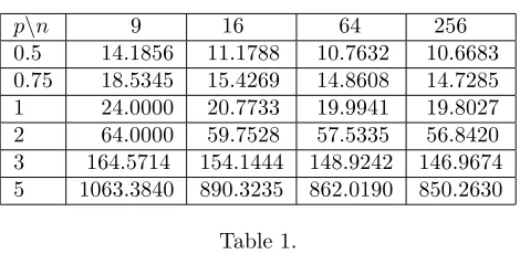
Ω in twodimension. These domains are the unit square, the ”unit circle” defined in (6), and the ”semicircle”, and the quadrant of the ”circle” with radius 1. The exact values for λ1 are known from [10] for the linear case (p= 1).In the tables
p\n 9 16 64 256 0.5 14.1856 11.1788 10.7632 10.6683 0.75 18.5345 15.4269 14.8608 14.7285
1 24.0000 20.7733 19.9941 19.8027
2 64.0000 59.7528 57.5335 56.8420
3 164.5714 154.1444 148.9242 146.9674 5 1063.3840 890.3235 862.0190 850.2630
Table 1.
In case p= 1 the known value is λ1(1) = 2π2≈19.7392. Our approximation
differs from the known value by 0.32 %. In case of square domain we can evaluate the relative error for any value of p since we have the formula (9). The relative error is less then 1 % when p∈[0.25,10].Similar formula is not known for the other domains. Thus we can compare the approximate solution with the exact solution only when p = 1. The approximate values are reported in Table 2 for the unit ”circle”.
p\n 67 227 835 3203
0.5 4.1774 4.0573 4.0277 4.0203
0.75 5.0962 4.9366 4.8978 4.8882
1 6.0646 5.8522 5.8004 5.7875
2 10.5134 10.0104 9.8780 9.8435
3 15.9061 15.0216 14.7739 14.7095 5 29.4856 27.6169 27.0521 26.8875
Table 2.
In the linear case the exact solution is 5.7831 [10]. Here the difference between the exact and finite element solution is 0.08 %. For the ”semicircle” The calculated values are presented in Table 3.
p\n 33 113 417 1601
0.5 8.2958 7.8851 7.7885 7.7645
0.75 11.5277 10.9784 10.8399 10.8066
1 15.7835 14.9546 14.7500 14.6989
2 50.7108 46.2403 44.9594 44.6189
3 150.3274 130.6471 124.0847 122.1544 5 1168.4845 921.3901 822.6043 788.0588
Table 3.
In the linear case the exact solution is given by 14.6842 [10]. The difference is here 0.1 %. The numerical results for λ1 when the domain is bounded by the
quadrant of the ”circle” are given in Table 4.
p\n 19 61 217 817
0.5 13.2191 12.1671 11.9362 11.8787
0.75 19.7591 18.3118 17.9715 17.8864
1 29.3712 27.1025 26.5555 26.4198
2 144.0884 120.3870 115.2347 113.9156
3 735.6182 504.7015 462.9082 451.2033
5 18610.8737 8298.0772 6753.8355 6269.8435
The known value is 26.3682 forp= 1, and the difference is 0.2 %.
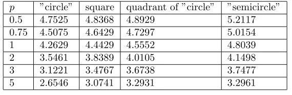
The following table gives the relative frequency in certain cases for the gravest tone of membranes under similar mechanical conditions and of equal area (Table 5.). We can conclude that for any value p from [0.5, 5] the ”circular” membrane has the gravest mode similarly as in the linear case [10].
p ”circle” square quadrant of ”circle” ”semicircle”
0.5 4.7525 4.8368 4.8929 5.2117
0.75 4.5075 4.6429 4.7297 5.0154
1 4.2629 4.4429 4.5552 4.8039
2 3.5461 3.8389 4.0105 4.1498
3 3.1221 3.4767 3.6738 3.7477
5 2.6546 3.0741 3.2931 3.2961
Table 5.
Acknowledgement 4 This work was supported by the National Research Founda-tion OTKA T026138. The author is grateful to the referee for his valuable comments and helpful
References
[1] G. Bogn´ar, The eigenvalue problem of some nonlinear elliptic partial differential equation,Studia Scie. Math. Hung., 29 (1994), 213-231.
[2] G. Bogn´ar, Existence theorem for eigenvalues of a nonlinear eigenvalue
prob-lem, Communications on Applied Nonlinear Analysis, 4, 1997, No. 2, 93-102.
[3] G. Bogn´ar, On the solution of some nonlinear boundary value problem,Proc. WCNA, August 19-26, 1992. Tampa, 2449-2458.
[4] P. G. Ciarlet,The Finite Element Method for Elliptic Problems, North-Holland, Amsterdam-New York-Oxford, 1979.
[5] G. Faber, Beweis, dass unter allen homogenen Membranen von gleicher Flache und gleicher Spannung die kreisf¨ormige den tiessten Grundton gibt, Sitz. ber. bayer. Akad. Wiss., 1923, 169-172.
[6] G. H. Hardy, J. E. Littlewood, G. Polya, Inequalities, Cambridge University Press, 1952.
[7] E. Krahn, ¨Uber eine von Rayleigh formulierte Minimaleigenschaft des Kreises, Math. Ann., 94 (1924), 97-100.
[8] E. Krahn, ¨Uber Minimaleigenschaften der Kugel in drei und mehr dimensionen, Acta Comm Univ. tartu (Dorpat), A9 (1926), 1-44.
[9] G. P´olya, G. Szeg˝o,Isoperimetric Inequalities in Mathematical Physics, Prince-ton Univ. Press, 1951.