On the breakup of slender liquid bridges: Experiments and a 1-D numerical analysis
A. Ramosa,*, F.J. Garcíaa,b, J.M. Valverdea
aDepartamento de Electrónica y Electromagnetismo, Universidad de Sevilla, Spain bDepartamento de Física Aplicada, Universidad de Sevilla, Spain
(Received 30 March 1998; revised 7 October 1998; accepted 20 October 1998)
Abstract – Slender axisymmetric dielectric liquid bridges are made stable by the action of an axial electric field. In this paper, the subsequent dynamics of a slender liquid bridge after turning off the electric field is considered. The evolution in time of the bridge profile is investigated both theoretically and experimentally. A one-dimensional model is used to simulate the dynamic response of the system. Experiments are performed applying an axial electric field to a liquid bridge of 1 mm of diameter, and turning-off the electric field. The evolution of the liquid bridge is recorded using a video camera, and the digitized images are analysed. Good agreement between computations and experiments is found.Elsevier, Paris
1. Introduction
The breakup of liquid bridges is a classical problem in fluid dynamics (Meseguer [1], Meseguer and Sanz [2], Zhang et al. [3]). This process is usually performed by either extracting liquid or separating the anchoring disks. Theoretical studies of the liquid bridge breakup have usually considered the evolution of an initial unstable shape with zero velocity (Meseguer [1], Meseguer and Sanz [2]). Also they have used one-dimensional models whose range of validity is restricted to large values of the slenderness of the liquid bridge. Here we show that the use of an electric field allows us to study this situation experimentally. The electric field is able to stabilize a slender liquid bridge in the presence of gravity, which would otherwise be unstable (González et al. [4], Ramos et al. [5]). After switching off the electric field, the liquid bridge breaks up. The initial condition corresponds to a shape that is unstable with zero velocity. The subsequent evolution is purely hydrodynamic, because the depolarization is instantaneous compared to any mechanical time. The experiments are recorded by using a video system, and the digitized images are analysed. In the experiments we have focused on castor oil, a liquid of high viscosity.
We have worked with small liquid bridges (anchoring disks of 1 mm diameter) to minimize the gravitational effects. To our knowledge, this is the first time that AC electric fields have stabilized liquid bridges with slenderness greater than the Rayleigh limit in the absence of an outer bath. Previous experiments (González et al. [4], Ramos et al. [5]) involved the use of an outer liquid of similar density, in order to diminish the gravitational forces. Now, a direct comparison with one-dimensional models is possible, since the liquid bridge is slender and there is no outer bath. The evolution of the liquid bridge is clearly influenced by the presence of a liquid bath when both liquids are almost inviscid (Sanz [6]), owing to inertial effects. However, in the particular case of a very viscous liquid bridge, the influence of an inviscid outer bath should be negligible. This would allow a comparison with the predictions of one-dimensional (1-D) models, but the experiments would be more complicated.
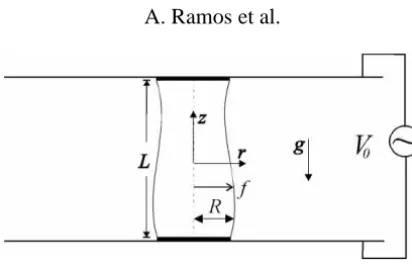
Figure 1. Schematic of the liquid bridge in our experiment.
The evolution of the bridge shape is investigated both numerically and experimentally. In the computations, 1-D models, based on the slender jet approximation, have been used to analyse the breaking process. The simplest one is the inviscid slice model, initially proposed by Lee [7], and afterwards generalized to inviscid liquid bridges by Meseguer [1]. Only recently, this model has been extended to viscous liquid columns (Eggers and Dupont [8], García and Castellanos [9], García and Castellanos [10]). Other more complex 1-D models, such as the Cosserat model (Bogy [11]), have been used in the same context. A wide review of the subject has been performed by Eggers [12]. Here, we have focused on the integration of the 1-D viscous slice model. However, some computations with other more complex 1-D models have been made for comparison. Good agreement between the 1-D viscous model predictions and experiments is found.
2. 1-D viscous model and numerical approach
The system under consideration is an axisymmetric liquid bridge of fixed volumeV, anchored between two disks of radiusR that are separated a distanceL. The liquid has density ρ, dynamic viscosity η, and surface tensionσ, which are supposed to be uniform and constant. The influence of the surrounding gas is neglected. The direction of the gravity vector g lies along the axis of symmetry. A cylindrical coordinate system is used, in whichzis the distance along the axis of symmetry andr is the distance to the axis (see figure 1).
Under the hypothesis of axisymmetry and large slenderness of the liquid bridge, the Navier–Stokes equations lead to a set of 1-D models (García and Castellanos [9], García and Castellanos [10]), the simplest of which is the viscous slice model. The nondimensional equations that define this model are three. The first comes from the balance of momentum in the vertical direction. The radial pressure equilibrium leads to the second equation, which equates the average pressure on a slice to the capillary pressure. Finally, the third equation is simply the mass conservation equation applied to a slice. These equations, which are obtained by averaging the original 3-D equations on a slice radially, are
wheret denotes time, and subscripts indicate partial derivative with respect to z ort. The functions w(z, t),
time, velocity, and pressure, respectively. The nondimensional numberC=η/(ρσ R)1/2, known as Ohnesorge
number, gives the relative weight of viscous forces against capillary ones. The other nondimensional number appearing in the equations is the Bond number, Bo=ρgR2/σ, which measures the gravitational force relative
to the capillary one.
The solution of the problem must also satisfy the following boundary conditions at the anchors:
w(±3, t)=0, (4)
f (±3, t)=1, (5)
where3=L/2Ris the slenderness of the liquid bridge, which is assumed to be large. Equations (4) stand for
the impenetrability of the anchoring disks, while equations (5) account for the anchoring of the liquid bridge to the edges of the supporting disks.
The necessary initial conditions are given by the experimental shape of the interface,F (z), while the initial velocity is zero:
f (z,0)=F (z), w(z,0)=0. (6)
The governing set of one-dimensional equations is solved numerically by using the Galerkin/Hermite finite element method (Strang and Fix [13]) for the discretization in z-coordinate (typically 32 elements) and an adaptive implicit finite difference scheme of second order for discretization in time (Gresho et al. [14]).
For the spatial discretization, the basis functions that we use to represent the unknowns are Hermite
cubics (Strang and Fix [13]). They are continuous and of continuous derivative, so they belong to a class
of interpolating functions known asC1 basis functions. They are suitable for problems with derivatives up
to 4. In our 1-D model, the highest-order derivative forf is 3, and forwis 2. Thus, these basis functions are appropriate. A formulation of the numerical problem that uses basis functions that are only continuous (C0basis functions) is shown by Zhang et al. [3]. However, they have to introduce a new variable and a new equation so that the highest-order derivative appearing in the equations is of second order. The domain−36z63
is divided inNe elements. In the Hermite formulation, each element has two double nodes placed at the two endpoints of the element. At each point the values of the function and its derivative should be specified. Thus, there are 2Ne+2 unknowns corresponding to the values of the function and its derivative at theNe+1 points of the grid. The unknownsf andware then expanded in terms of a series of Hermite basis functionsgi(z):
f (z, t)=
The Galerkin weighted residuals of Eqs (1) and (3) are constructed by weighting each equation by the basis functions and integrating the resulting expressions over the computational domain. The weighted residuals are next integrated by parts to reduce the order of the highest-order derivative appearing in them, and the resulting expressions are then simplified because of boundary conditions. The resulting discrete equations are
The Galerkin weighted residuals are a set of nonlinear ordinary differential equations in time. Time derivatives are discretized by either first-order backward difference or second-order trapezoid rule. The solution at each time step of the resulting nonlinear algebraic equations is solved by Newton iteration. Five backward difference time steps provide the necessary smoothing at the beginning of the computations (Zhang et al. [3]). The subsequent time steps employ the trapezoid rule. In addition, a predictor–corrector scheme is used that allows us to estimate the local time truncation error: an explicit Euler predictor with the first-order backward difference corrector, and a second-order Adams–Brashforth predictor with the trapezoid rule. The time step is chosen adaptively by requiring a specified time truncation error as outlined in Gresho et al. [14]. In a typical run describing a breakup, about 30 time steps are necessary to achievefmin≃10−2(fmin, the radius of the neck
of the shape), with an accuracy per time step of 10−3.
3. Experimental approach
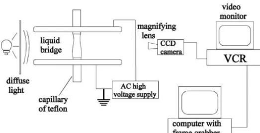
The liquid bridge is held captive between two capillaries of 0.53 mm radius, that are in the center of two parallel metallic plates (see figure 2). The capillaries are made of teflon and the liquid employed is castor oil. Liquid is supplied by a syringe. An AC potential difference is applied between the metallic plates, which allows us to hold a slender liquid bridge. Typical rms values of the electric field that we have applied are about 10 kV/cm, limited in practice by the electrical breakdown of air. Typical values of the slenderness3that we have studied range from 2.6 to 3.5. Much larger elongation of the liquid bridge by means of the AC electric field would require the use of an artificial atmosphere of a gas with higher dielectric strength.
In the presence of gravity, liquid bridges with these values of3are unstable if the axial electric field is not applied. The stabilizing mechanism of the applied electric field is obtained in the perfect dielectric limit, i.e. with negligible free-charge currents (González et al. [4], Ramos et al. [5]). Since there is always a residual conductivity in the liquids, it is normal to use AC fields to avoid the accumulation of free charges on the interfaces. The driving frequency of the AC potential should be much greater than the inverse of the charge relaxation time. In our case, ω=2πf (f =100 Hz) is much greater than σe/ε=7.2 s−1, withσe and ε the
electrical conductivity and permittivity, respectively, of castor oil (Ramos et al. [5]). The frequencyωis also much greater than the inverse of the typical evolution time, which is of the order of 0.1 s. In this way, the liquid bridge shape does not follow the frequency of the applied electric field and static liquid bridges can be held. When the potential difference is switched off, in a time much shorter than the typical evolution time of the bridge, the liquid column has a shape that is unstable with a zero initial velocity field.
Figure 3. Evolution in time after turning off the potential difference of a castor oil bridge with a volume of 3 mm3and a slenderness of3=3.0.
The subsequent evolution is video-taped, and the digitized images are analysed. The camera records 25 images per second. The images are digitized by a frame grabber, an image acquisition board (TARGA+), which is installed in a PC. An edge detection routine is employed to locate the interfacial profile from the digitized images. In figure 3, we can see the profiles corresponding to a given experiment.
We have used castor oil in our experiments because of the high value of its viscosity. In this way, the liquid bridge breakup takes about half a second, thus allowing us to grab around 10 images of the evolution process. For liquids with lower values of viscosity, the evolution process takes much shorter times, and we would need an ultra-high speed video system. The viscosity of the castor oil as a function of temperature was measured using a viscometer (Brookfield LVTDV-II+). In the range of temperature from 20 to 30◦C, the measured values
of the viscosity can be fitted by a quadratic function of temperature
η=2.187×(T −25)2−51.70×(T −25)+681.7 cp,
with less than 1% of uncertainty. These values compare well with others in the literature. The viscosity of castor oil shows a strong dependence on temperature: it varies from 995 cp atT =20◦C to 477 cp atT =30◦C. This
variation with temperature allows us to study the breakups with different viscosities.
The density value of castor oil is 0.958 g/cm3atT =25◦C and decreases with temperature by about 0.05%
per degree (Ramos et al. [5]).
To measure the surface tension of the air–liquid interface, we have compared the equilibrium shapes of stable pendant drops of castor oil, with numerical solutions of the Laplace equation for different Bond numbers (a pendant drop method). The value obtained was σ =0.0318±0.0015 N/m. Similar values are found in the literature. From this value of the surface tension, the liquid bridge breakups were performed under a gravitational Bond number of Bo=0.0825±0.004. The Bond number was also obtained from a comparison
of the experimental profiles of stable liquid bridges with our computations for them in the presence of gravity (Ramos and Castellanos [15]). The value of the Bond number that we got in this case was around Bo=0.08–
4. Results and discussion
We have focused on the evolution in time of the neck of the bridge, i.e. the minimum value off (z) as a function of time. For each numerical comparison, the initial condition is the experimental shape before the electric field is switched off.
Figures 4, 6, and 7 show the neck radius fmin (made nondimensional with R) as a function of time (in seconds) for three different temperature conditions. We expect noticeable changes in the Ohnesorge number
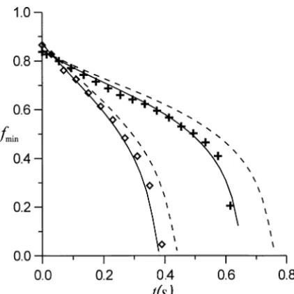
Figure 4. Neck radius versus time for two different initial conditions atT=22.8◦C:(+) 31=2.65 andτ1=1.01;(⋄) 32=3.0 andτ2=1.08. Solid
line theoretical curve.
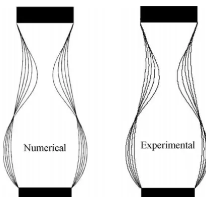
Figure 5. Numerical (left) and experimental (right) shapes of the evolution in time of a liquid bridge of3=3.0 fort=0,0.08,0.16,0.24,0.32 s, where
Figure 6. Neck radius versus time for two different initial conditions atT=25.1◦C:(+) 31=3.1 andτ1=1.19;(⋄) 32=3.45 andτ2=1.46.
Figure 7. Neck radius versus time for two different initial conditions atT=24.5◦C:(+) 31=2.8 andτ1=1.13;(⋄) 32=3.0 andτ2=1.24.
(due to viscosity variations) but not in the Bond number. For the computations we have fixed the Bond number to Bo=0.082.
In figure 4 we show fmin versus time for an experiment with temperature T =22.8◦C (η=806 cp). The
value of the Ohnesorge number that fits the experimental data isC=7.3. This value is 15% greater than the
experimental value obtained fromCexp=η/(ρσ R)1/2=6.33. However, only one curve is used for this fitting,
the other one fits automatically. We will comment later on the small discrepancy. The breakups correspond to two different values of the slenderness: 31=2.65 and 32=3.0. In both cases the volumes are close to the case of a cylinder of the same height and radius: τ1=1.01 and τ2=1.08, where τ ≡V /(π R2L) (note
and E2=10.8 kV/cm. The fastest evolution corresponds to the case of 32=3.0, which can be explained
because the initial condition corresponds to a more unstable shape. In figure 5 we show a comparison between experimental and numerical profiles for the case labelled as 2 in figure 4.
Figure 6 showsfminversus time in an experiment with temperature T =25.1◦C (η=677 cp). The value of
the viscosity in this case should be lower than in the previous case. The breakups correspond to two different values of the slenderness31=3.1 and32=3.45, and volumes τ1=1.19 andτ2=1.46. The rms values of the electric field for holding the liquid bridge areE1=10.0 andE2=12.3 kV/cm. Again, the fastest evolution
corresponds to the case of greater 3. The continuous lines show the numerical results for Bo=0.082 and
C=6.1. For this comparison, we have decreased the value ofC according to the dependence of the viscosity
with temperature. That is, we have dividedC=7.3 by the viscosity value forT =22.8◦C and multiplied it by
the viscosity value atT =25.1◦C. The dashed lines show the behaviour offminif the Ohnesorge number were
not changed with temperature, i.e. forC=7.3, according to the 1-D model. Clearly, the lower the viscosity,
the faster is the evolution.
Figure 7 shows fmin versus time in an experiment with temperature T =24.5◦C (η=708 cp). Changing
the value of the Ohnesorge number according to the temperature dependence of viscosity we getC=6.3. The
rms values of the electric field for holding the two liquid bridges areE1=9.25 and E2=11.4 kV/cm, with
slenderness31=2.8 and32=3.0 and volumes τ1=1.13 andτ2=1.24. The dashed line shows what would
have been the evolution if the Ohnesorge number had beenC=7.3 instead of 6.3, according to the 1-D model.
The values that we get for the Ohnesorge number from the numerical calculations are 15% greater than the actual values. However, once we have chosen a value for a given breakup, the other breakups are described reasonably well. A possible explanation for this discrepancy is that small errors in the determination of the experimental shapes can lead to great errors in the breakup time. We have verified numerically that a 3% error in the determination of the slenderness of the bridge can lead to a 15% error in the breakup time. Thus, if the liquid bridges shapes were less slender than the ones we have determined by the edge detection routine, by a factor of 3%, the breakup times would correspond to lower values of the Ohnesorge number.
In all these numerical computations we have used the viscous slice model. One could wonder what are the errors associated with this model, and whether these errors are responsible or not for the observed systematic discrepancy. A first estimate of the error in the breaking time comes from a comparison of the growth rates given by the linear 3-D and 1-D analysis of cylindrical liquid bridges in the absence of gravity (García and
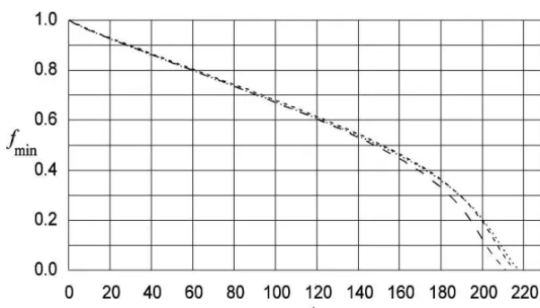
Castellanos [10]). From this comparison, the expected error would be about 3% for very viscous liquid bridges of slenderness around 3. So as to test this estimate, we have performed a numerical simulation of the rupture of a cylindrical liquid bridge with3=3, C=7.3, and Bo=0.082, using three different models (viscous slice,
averaged, and parabolic) developed by García and Castellanos [10]. As for the linear results, the differences among the breaking times given by the different models provide an estimate of the error. As shown in figure 8, where the evolution offminis plotted versus the nondimensional time, the differences between breaking times predicted by these three models are of the order of 3%. This supports our expectation that the discrepancies are not due to the viscous slice model.
5. Conclusions
In this paper we have shown experimentally that the use of a stabilizing electric field allows a study of the breakup of long liquid bridges in the presence of gravity, without the aid of an outer liquid bath. After switching off the electric field, the liquid bridge breaks up spontaneously. The subsequent evolution is purely hydrodynamic, with an initial condition that corresponds to a shape that is unstable with zero velocity. The comparison with one-dimensional models is now possible, because there is no outer bath and the liquid bridges are long, two conditions that the 1-D models require to be applicable with confidence.
For the comparison with the one-dimensional model, we have analysed breakups of liquid bridges with high values of viscosity (high values of the Ohnesorge number). The comparison with the 1-D viscous slice model is satisfactory. Both experiments and numerics show us that, for a given initial unstable shape, the breakup time increases with the Ohnesorge number; and decreases with the Bond number and the slenderness, as should be expected.
We would also like to stress the small computational effort necessary to describe a breakup using the one-dimensional models, that is several orders of magnitude more economical than using the full Navier–Stokes equations.
This study is a first step in a wider parametric analysis of the dynamics of liquid bridges that will include the effect of electric fields.
Acknowledgements
We acknowledge Dr. J.M. Perales for providing us with part of the experimental apparatus. We also acknowledge fruitful discussions with Prof. A. Castellanos and technical assistance from Taller de la Facultad de Física de Sevilla. This work was carried out with financial support from DGICYT (Spanish Government Agency) under contract PB96-1375.
References
[1] Meseguer J., The breaking of axisymmetric slender liquid bridges, J. Fluid Mech. 130 (1983) 123.
[2] Meseguer J., Sanz A., Numerical and experimental study of the dynamics of axisymmetric slender liquid bridges, J. Fluid Mech. 153 (1985) 83. [3] Zhang X., Padgett R.S., Basaran O.A., Nonlinear deformation and breakup of stretching liquid bridge, J. Fluid Mech. 329 (1996) 207. [4] González H., McCluskey F.M.J., Castellanos A., Barrero A., Stabilization of dielectric liquid bridges by electric fields in the absence of gravity,
J. Fluid Mech. 206 (1989) 545.
[5] Ramos A., González H., Castellanos A., Experiments on dielectric liquid bridges subjected to axial electric fields, Phys. Fluids 6 (1994) 3206. [6] Sanz A., The influence of the outer bath in the dynamics of axisymmetric liquid bridges, J. Fluid Mech. 156 (1985) 101.
[8] Eggers J., Dupont T.F., Drop formation in a one-dimensional approximation of the Navier–Stokes equation, J. Fluid Mech. 262 (1994) 205. [9] García J., Castellanos A., One dimensional models for slender axisymmetric viscous liquid jets, Phys. Fluids 6 (1994) 2676.
[10] García J., Castellanos A., One dimensional models for slender axisymmetric viscous liquid bridges, Phys. Fluids 8 (1996) 2837. [11] Bogy D.B., Drop formation in a circular liquid jet, Ann. Rev. Fluid Mech. 11 (1979) 207.
[12] Eggers J., Nonlinear dynamics and breakup of free-surface flows, Rev. Mod. Phys. 69 (3) (1997) 865. [13] Strang G., Fix G.J., An Analysis of the Finite Element Method, Prentice-Hall, Englewood Cliffs, NJ, 1973.
[14] Gresho P.M., Lee R.L., Sani R.L., On the time dependent solution of the incompressible Navier–Stokes equations in two and three dimensions, in: Recent Advances in Numerical Methods in Fluids, Vol. 1, Pineridge, Swansea, 1979, p. 27.
[15] Ramos A., Castellanos A., Bifurcation diagrams of axisymmetric liquid bridges of arbitrary volume in electric and gravitational axial fields, J. Fluid Mech. 249 (1993) 207.