An Innovative Heuristic for Joint Replenishment Problem
with Deterministic and Stochastic Demand
Yugowati Praharsi1a, Hindriyanto Dwi Purnomo2a Hui-Ming Wee3b, Department of Information Technology,
Satya Wacana Christian University, Indonesia a Department of Industrial and System Engineering,
Chung Yuan Christian University, Taiwan b
Corresponding Author: [email protected]
Abstract
Joint replenishment problem (JRP) is a common real problem which aims to minimize order cost and inventory holding cost. In this paper, classical, centralized and decentralized JRP models are discussed. An innovative heuristic to minimize the total cost is implemented for each model. This heuristic seeks to balance the order cost and the inventory holding costs. The results show that the innovative heuristic can best be implemented in the classical and decentralized models. For stochastic demand such as Poisson or Exponential distribution, the innovative heuristic can be implemented with the random variables which are generated by Monte Carlo simulation.
Keywords: Innovative Heuristic, Joint Replenishment Problem, Stochastic Demand, Monte Carlo Simulation
1. Introduction
Joint replenishment problem (JRP) is a common practical problem where a group of items is replenished simultaneously. Its applications include ordering multi items from a single supplier, and production of a family of items at a single facility. JRP has been developed intensively recently to minimize the order cost and the inventory holding cost (Hoque, 2006). JRP may lead to cost saving due to the reduction of the major ordering cost. The JRP’s total cost is composed of two parts: 1) setup or ordering cost; for retailer, 2) holding cost. The cost of placing an order for a number of different items has two components: 1) a major ordering cost; it is independent to the items that are ordered and 2) a minor ordering cost; it is dependent to the particular item that is ordered.
heuristics. An innovative heuristic procedure balances the replenishment/order/setup cost and inventory holding costs for different items in an iterative procedure (Abdul-Jalbar, Segerstedt, Sicilia, & Nilsson, 2010; Nilsson et al., 2007).
The objectives of this research are: 1) to derive three JRP mathematical models: classical, centralized and decentralized models; 2) to develop innovative heuristic procedure for models with deterministic and stochastic demand. We show how the innovative heuristic approach can minimize the total cost.
The remaining parts of this paper are organized as follows. Notation and assumption is given in section 2. The classical, decentralized, and centralized JRP models are described in section 3, 4, and 5, respectively. An innovativeheuristic procedure is presented in section 6 and stochastic demand and its implementation are given in section 7. Finally, experimental results and some conclusions are summarized in section 8 and 9, respectively.
2. Notation and Assumption
The following notations are used in this paper:T : Time between successive replenishments (years)
S : Major ordering cost associated with each replenishment ($/order)
TC : Total annual holding and ordering costs for all the products ($/year)
i : 1, 2, …, n, a product index
n : Number of products
Di : Annual demand for product i (units/year)
hi : Annual holding cost of product i ($/unit/year)
si : The minor ordering cost incurred if product i is ordered in a replenishment ($/order)
Qi : the ratio between the two costs for item- i
Ti : Time interval between successive replenishment of product i (years)
ki : The integer number of T intervals that the replenishment quantity of item i will last
Under the Indirect Grouping Strategy (IGS), the cycle time for every product is an integer multiple ki of the replenishment cycle time T. Thus, the cycle time for product i is Ti =
ki T. In this research, strict cycle policies is used in which at least one item is ordered at every replenishment opportunity, so that ki 1.
3. Classical JRP Model
The assumptions of classical JRP model are similar to the economic order quantity (EOQ) model. The total cost for the retailer per unit time is (Khouja & Goyal, 2008):
(1)
The optimal time interval,T*, that minimizes Eq. (1) with a given set of k
1, k2, …, kn
is :
(2) Substituting optimal T* into Eq. (1) gives the total cost function, which depends only on the
set of kivalues as:
(3)
The replenishment cost and inventory holding cost for item i:
4. Decentralized System
In the decentralized replenishment, each entity within the supply chain focuses on minimizing its own costs. The retailer makes the replenishment decision for each item based on the EOQ. The major component of setup cost is a fixed transportation cost, regardless of items ordered, and the minor setup costs are order-processing costs for specific items included in the order (J.-M. Chen & T.-H. Chen, 2005). The total cost of n items per unit time for the retailer is:
(8)
The optimal time interval,T*, that minimizes Eq. (8) with a given set of k1, k2, …, kn
is :
(9)
Substituting optimal T* into Eq. (8) gives the total cost function, which depends only on the set of kivalues:
The replenishment cost and inventory holding cost for item i respectively are:
(11)
(12)
(14)
5. Centralized System
In the centralized policy, multi-item replenishment is coordinated using a common replenishment cycle for all items, which reduced the frequency of major setups for the retailer. The major setup cost incurred by the retailer is reduced from n to one, due to joint replenishment among a family of items (J.-M. Chen & T.-H. Chen, 2005). The total cost for the retailer per unit time is:
(15)
The optimal time interval,T*, that minimizes Eq. (15) can be found after taking the derivative of TC with respect to T and equaling the result to zero, resulting in:
(16)
Substituting optimal T* into Eq. (15) gives the total cost function:
(17)
The replenishment cost and inventory holding cost for item i respectively are:
(18)
(19)
SubstituteT*to i
Q , one has:
(21)
6. An Innovative Heuristic Procedure
The innovative heuristic procedure balances the replenishment/order cost and inventory holding costs for different items in an iterative procedure. The JRP has the same concept as the traditional EOQ for an individual item. The ratio between the replenishment cost and the inventory holding cost without any safety stock is equal to one. The smaller the ratio, the higher the cost. The closer the individual ratio to one, the better the solution.
In order to adjust the ratio closest to one, two-steps of heuristic is needed. In the heuristic step, the step starts by setting the ki values to one (all items are replenished every time interval). Then, check the ratios and track how the total cost changes as the replenishment frequencies (ki values) are updated (Nilsson et al., 2007).
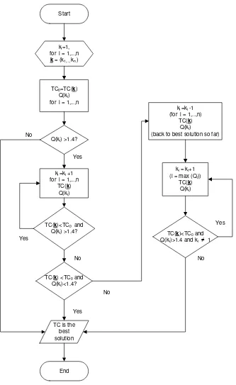
The detail of the innovative heuristic procedure is presented in Figure 1. The steps are given below:
1. Set all values of ki to 1, and compute the total cost for the initial solution.
2. Compute Qi and increase the values of ki by one for all items with ratios higher than 1.4. 3. Calculate the total cost. Repeat until all ratios are below 1.4 or the total cost start to
increase.
4. If all ratios are below 1.4, then we have derived the best solution for the total cost. 5. If the total cost start to increase, the best solution is the previous iteration.
6. Choose the highest Qi. Then increase ki value one by one for ith item.
7. Calculate the total cost and ratios. Repeat this until all quotients are below 1.4.. If there is
ki=1, then it must be skipped.
8. If all ratios are below 1.4 excluding the exception, then we got the best solution for the total cost.
The value 1.4 is chosen because it produces the lowest error (Nilsson et al., 2007). Nilsson already tested for 48,000 simulated test problems with the value of ratios ranging from 1.0 to 2.0.
7. Stochastic demand
There is significant uncertainty when retailer has to forecast or estimate customer demand. Inmost business activities, it is too complex to solve planning and processing using analytical solution. Recently, several coordinated replenishment policies for stochastic
) (
1 1
i i n
i i n
i i i i i
D h s S
demands are suggested in the literature (Kiesmuller, 2009). Monte Carlo can be used for stochastic demand with random variables. The flow chart diagram to implement the innovative heuristic using random variates is generated by Monte Carlo simulation for Poisson and Negative Exponential distribution. It is given in Figure 2.
Start
ki=1,
for i = 1,..,n k = (k1,...,kn )
TC0=TC(k)
Q(ki)
for i = 1,..,n
Q(ki) >1.4?
ki =ki +1
for i = 1,..,n TC(k)
Q(ki)
Yes
TC(k)<TC0 and
Q(ki) >1.4?
Yes
TC(k) <TC0 and
Q(ki)<1.4?
No
Yes
TC is the best solution No
No
ki =ki -1
(for i = 1,..,n) TC(k)
Q(ki)
(back to best solution so far)
ki = ki+1
(i = max (Qi))
TC(k) Q(ki)
TC(k)<TC0 and
Q(ki)>1.4 and ki ≠ 1
Yes
No
End
Define an input domain (Poisson/ Exponential) and number of forecasting
periods (N) d = 0
Generate Inputs randomly for several items by Monte Carlo Simulation
Set d= d + 1
1. Set the ki values are to one
2. Compute quotient (Qd(i)) and the Total Cost (TCd) using the innovative heuristic procedure
d <=N?
Yes
Sum = TCd
for d = 1,…, N
No
Figure 2.Anew heuristic implementation in Monte Carlo simulation
8. Result & Discussion
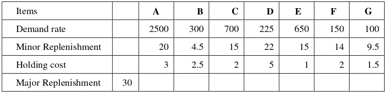
A numerical example is presented in Table 1. There are 7 items where demand rate, minor replenishment cost, holding cost, and major replenishment cost are known.
Table1. Initial Data (Nilsson et al., 2007)
Items A B C D E F G
Demand rate 2500 300 700 225 650 150 100
Minor Replenishment 20 4.5 15 22 15 14 9.5
Holding cost 3 2.5 2 5 1 2 1.5
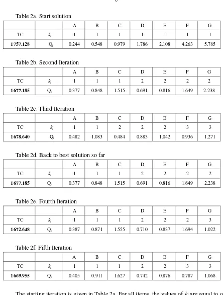
8.1 Results for Classical Model
The results for classical JRP model are given in Table 2a to Table 2f.
Table 2a. Start solution
A B C D E F G
TC ki 1 1 1 1 1 1 1
1757.128 Qi 0.244 0.548 0.979 1.786 2.108 4.263 5.785
Table 2b. Second Iteration
A B C D E F G
TC ki 1 1 1 2 2 2 2
1677.185 Qi 0.377 0.848 1.515 0.691 0.816 1.649 2.238
Table 2c. Third Iteration
A B C D E F G
TC ki 1 1 2 2 2 3 3
1678.640 Qi 0.482 1.083 0.484 0.883 1.042 0.936 1.271
Table 2d. Back to best solution so far
A B C D E F G
TC ki 1 1 1 2 2 2 2
1677.185 Qi 0.377 0.848 1.515 0.691 0.816 1.649 2.238
Table 2e. Fourth Iteration
A B C D E F G
TC ki 1 1 1 2 2 2 3
1672.648 Qi 0.387 0.871 1.555 0.710 0.837 1.694 1.022
Table 2f. Fifth Iteration
A B C D E F G
TC ki 1 1 1 2 2 3 3
1669.955 Qi 0.405 0.911 1.627 0.742 0.876 0.787 1.068
solution so far (Table 2b). Iteration is then continued by increasing ki for the largest quotient value (Table 2e). The final solution is obtained by the fifth iteration (Table 2f). The total cost for the classical model of JRP is $1669.955. The iteration stopps because there is no ratios value which is larger than 1.4.
8.2 Results for the Centralization System
The result for centralized system is the same as in Table 2a, because the centralization system does not depend on ki values. In other words, by setting the values of ki equal to one, the total cost of the starting solution for classical model will be the same as the total cost of the centralized system in Eq. (15).
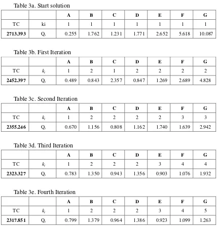
8.3 Results for the Decentralized system
The results for the decentralization system are given in Table 3a to Table 3e.
Table 3a. Start solution
A B C D E F G
TC ki 1 1 1 1 1 1 1
2713.393 Qi 0.255 1.762 1.231 1.771 2.652 5.618 10.087
Table 3b. First Iteration
A B C D E F G
TC ki 1 2 1 2 2 2 2
2452.397 Qi 0.489 0.843 2.357 0.847 1.269 2.689 4.828
Table 3c. Second Iteration
A B C D E F G
TC ki 1 2 2 2 2 3 3
2355.246 Qi 0.670 1.156 0.808 1.162 1.740 1.639 2.942
Table 3d. Third Iteration
A B C D E F G
TC ki 1 2 2 2 3 4 4
2323.327 Qi 0.783 1.350 0.943 1.356 0.903 1.076 1.932
Table 3e. Fourth Iteration
A B C D E F G
TC ki 1 2 2 2 3 4 5
Starting iteration is given in Table 3a. For all items, the values of ki are set to one. It means at least one item is ordered for every replenishment opportunity. The iteration is continued by looking for ratios values which are larger than 1.4. Then, ki values are added by one.
The final solution is obtained in the fourth iteration (Table 3e). The total cost for the decentralized system is $2317.851. The iteration stopps because there is no quotient value larger than 1.4. So, we do not need to continue to the next iteration or to increase the values of ki.
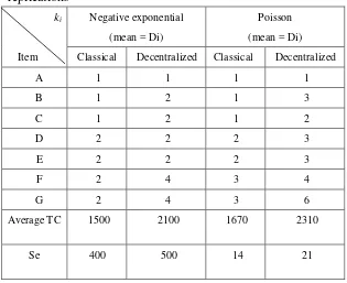
8.4 Results for the Stochastic Demand
The results for the stochastic demand with negative exponential and the Poisson distributions are shown in Table 4 and 5, respectively. The experiment is done for 1000 replications.
Table 4.The results of the negative exponential and the Poisson distribution for 1000 replications
ki
Item
Negative exponential
(mean = Di)
Poisson
(mean = Di)
Classical Decentralized Classical Decentralized
A 1 1 1 1
B 1 2 1 3
C 1 2 1 2
D 2 2 2 3
E 2 2 2 3
F 2 4 3 4
G 2 4 3 6
Average TC 1500 2100 1670 2310
Se 400 500 14 21
9. Conclusion and Future Work
In this paper, an innovative heuristic is developed to offer a different approach to solve a joint replenishment problem. The innovative heuristic can be implemented for classical as well as for the decentralized models. The easily understood spreadsheet application by an independently owned retailer who uses the decentralized distribution strategy can easily be used. For the centralized policy, the innovative heuristic does not work well because the policy does not use an integer multiple ki. For stochastic demand such as Poisson or Negative Exponential distribution, the innovative heuristic can be implemented in random variates which are generated by Monte Carlo simulation. In addition, Poisson distribution describes the demand at retailer level better because the results are similar to the analytic solution.
References
Abdul-Jalbar, B., Segerstedt, A., Sicilia, J., & Nilsson, A. (2010). A new heuristic to solve the one-warehouse N-retailer problem. Computers and Operations Research, 37, 265-272. Chen, J.-M., & Chen, T.-H. (2005). The multi-item replenishment problem in a two-echelon
supply chain: the effect of centralization versus decentralization. Computers and Operations Research, 32, 3191-3207.
Chen, T.-H., & Chen, J.-M. (2005). Optimizing supply chain collaboration based on joint replenishment and channer coordination. Transportation Research Part E, 41, 261-285. Hoque, M. A. (2006). An optimal solution technique for the joint replenishment problem with
storage and transport capacities and budget constraints. European Journal of Operational Research, 175, 1033-1042.
Khouja, M., & Goyal, S. (2008). A review of the joint replenishment problem literature: 1989-2005. European Journal of Operational Research, 186, 1-16.
Kiesmuller, G. P. (2009). A multi-item periodic replenishment policy with full truckloads.
International Journal of Production Economics, 118, 275-281. Lilja, D. J. (2000). Probability Distributions. 2009, from
http://www.iohk.com/UserPages/erictang/probability.html
Lordanova, T. (2009). Introduction to Monte Carlo Simulation. from
http://www.investopedia.com/articles/07/monte_carlo_intro.asp
Nilsson, A., Segerstedt, A., & Sluis, E. v. d. (2007). A new iterative heuristic to solve the joint replenishment problem using a spreadsheet technique. International Journal of