q
We are extremely grateful to Ken Judd and to Luis Puch for their most stimulating suggestions. The numerical computations have been performed on the Convex Exemplar SPP-1600 of the UniversiteH Catholique de Louvain. R. Boucekkine has been supported by a Grant&Actions de Recherche ConcerteHc' of the Ministry of Scienti"c Research of the Belgian French speaking community.
*Corresponding author. Tel.:#32 10 47 39 48; fax:#32 10 47 39 45.
E-mail address:[email protected] (R. Boucekkine). 25 (2001) 655}669
Numerical solution by iterative methods
of a class of vintage capital models
qRaouf Boucekkine
!
,
*
, Marc Germain
"
, Omar Licandro
#
,
Alphonse Magnus$
!Universite& Catholique de Louvain, IRES, Place Montesquieu, 3, B-1348 Louvain-la-Neuve, Belgium
"CORE, Louvain-la-Neuve, Belgium
#FEDEA, Madrid, Spain
$UCL, Louvain-la-Neuve, Belgium
Received 15 December 1997; accepted 2 September 1999
Abstract
We build up an iterative numerical procedure in order to solve vintage capital growth models with nonlinear utility functions and Leontie! technologies, a class of models intensively used in the literature since the early 1990s. The numerical procedure is of the relaxation type and uses a step-by-step maximization scheme for updating. The procedure is close to the cyclic coordinate descent algorithm as described in the computational mathematics literature. We explain why and how our numerical scheme is suitable to handle the considered class of models. ( 2001 Elsevier Science B.V. All rights reserved.
JEL classixcation: C63; E32; O40
Keywords: Vintage capital models; Relaxation; Optimization; Cyclic coordinate descent algorithm
1Creative destruction re#ects the idea that economic growth is mainly guided by successive innovations leading to the&death'of the resulting less productive techniques and equipment. 1. Introduction
The analysis of vintage capital growth models has regained interest since the early 1990s. Indeed, this kind of models allows to address quite conveniently many of the current key economic issues like investment volatility, equipment replacement and the general consequences of the schumpeterian creative destruction process.1 Investment volatility and equipment replacement are analyzed using vintage capital models by Benhabib and Rustichini (1993) and by Boucekkine et al. (1997a, 1998, 1999). Using the same framework, Aghion and Howitt (1994) and Caballero and Hammour (1996), among others, have ana-lyzed the e!ects of creative destruction on unemployment and job reallocation. Except in Benhabib}Rustichini's paper in which a general CES production function is adopted, all the previous contributions use a Leontie!technology. That is this type of technologies with complementary production factors straightforwardly ensures an endogenous determination of the equipment re-placement decision, while gross substitutability may directly induce in"nite optimal lifetimes for equipment, which sounds unrealistic. Moreover, when the utility functions are linear, Leontie! technologies allow to bring out some analytical results as in Boucekkine et al. (1997a).
As the latter treatment seems at best only implementable on di! erential-di!erence systems driven by periodic forcing functions, it is not general. One way to overcome the problem arising from the simultaneous occurrence of state dependent leads and lags consists in tackling the optimization problem directly without using the optimality conditions (where precisely the endogenous leads appear). The optimization work can be performed step by step within a standard "xed-point relaxation algorithm. This strategy is applied by Boucekkine et al. (1998) for example. Indeed, this device can be applied to a large class of vintage models of the recent economic literature, especially those including a Leontie! technology (like those quoted above for example). For convenience, we prefer to focus on this class of models since the speci"cations have been extremely popular in this decade.
Indeed, as it will be clear later, our method is also suitable to handle vintage capital models with non-Leontie! production functions, for example with putty-clay technologies as in Caballero and Hammour (1998) who use an ex ante CES function. According to the interpretation of these authors, this kind of ex ante production function can be thought of as an envelope of possible Leontie!functions whose technologies can be developed ex post. Therefore, it is not surprising at all that the technical problems involved in such cases are almost identical to those we face when dealing with vintage capital models with Leontie!technology. As for the issues related to the numerical resolution of the latter models when preferences are nonlinear, our approach has three important advantages:
(i) As explained just above, it allows to avoid the numerical di$culties coming from the simultaneous presence of endogenous leads and lags.
(ii) As theoretically and numerically shown in Boucekkine et al. (1997a, 1998), vintage capital models may give rise to corner and nondi!erentiable solu-tions. These features are obviously likely to be captured by an optimization algorithm based on the objective function. The relaxation algorithms so far used in the economic literature cannot do so because they usually handle the"rst order necessary conditions for interior solutions to exist.
(iii) Last but not least, our optimization device can be seen as an application of the cyclic coordinate descent algorithm as described by Luenberger (1965, Section 7.8), for example. Depending on the model under consideration, numerous variations of this algorithm can be considered to improve the e$ciency and reliability of the computational setting if necessary.
2All the properties of the model stated in this section are taken from Boucekkine et al. (1998). 2. Optimization problem
Consider a centrally planned closed economy characterized by a clay}clay vintage capital technology, i.e., technical progress is embodied in new machines. These new machines are of the Leontie!type, and the scrapping of old machines is endogenous. The central planner is supposed to maximize social welfare by solving the following problem:
max="
P
= 0u[c(t)] expM!otNdt (1)
subject to
y(t)"
P
t t~T(t)i(z) dz (2)
P
t t~T(t)i(z) expM!czNdz"1 (3)
y(t)"c(t)#i(t) (4)
04i(t)4y(t)
giveni(t) for allt(0.c(t) is consumption,y(t) is production,i(t) is investment and¹(t) represents the age of the oldest operating machines, orscrapping time. The utility function u(c) is assumed to be increasing and strictly concave. Parameter o is strictly positive and represents the rate of time preference. Machines fromvintaget, ∀t, are supposed to produce one unit of output each, and do require exp(!ct) units of labor. The parameter c is positive and represents (Harrod neutral) technical progress. Total labor resources are assumed to be constant and equal to one. (2) is the Leontie!production function and (3) is the equilibrium condition on the labor market.
A necessary condition for an interior solution of this optimization problem to exist is:2
u@(c(t))"
P
t`J(t) t(1!ec(z~t~T(z)))u@(c(z))e~o(z~t)dz (5)
while (2) and (3) capture its backward-looking dimension. Di!erentiating all these equations with respect to time yields an integro-di!erential-di!erence system with an endogenous lag ¹(t) and an endogenous leadJ(t). No robust solver is so far available to handle this kind of systems. The next section presents an iterative method allowing to solve the considered optimization problem. The optimization work relies directly on the objective function, so it does not use explicitly the necessary conditions that cause the simultaneous presence of endogenous leads and lags to occur.
Before, let us brie#y present the major dynamic property of this kind of models in order to allow the reader to understand the results of our experiments in Section 4. Because new machines are more productive in our model, older machines are optimally scrapped to be replaced by the former. The resulting dynamics follow the so-called&echo principle', i.e. the ability of an economy to reproduce its own past history (see Benhabib and Rustichini (1993) for a compre-hensive analysis of this feature). In addition to that, the example model considered in this paper admits a balanced growth path. When the economy starts with a too high (resp. low) past investment pro"le with respect to the balanced growth paths values, the adjustment to these balanced growth paths optimally induces an initial depression (resp. expansion) of investment, which will be reproduced in the future according to the&echo principle'. These echo oscilla-tions are indeed damped to allow convergence to the balanced growth paths.
3. Maximization by iteration:Numerical setting and theoretical justi5cations
3.1. The numerical setting
We decide to perform the approximate maximization of =, with
c(t)"y(t)!i(t) by (4), by replacing the unknown functionsiandyby piecewise constant functions on the intervals (0,D), (D, 2D),2. Leti0, i1,2; y0, y1,2be the unknown values. Piecewise constant functions would be crude and not very satisfactory approximations to well-behaved smooth functions, but we want to be ready to cope with possibly discontinuous solutions, and prefer to make a robust and unsophisticated choice. Then,y!iandu(y!i) still are piecewise constant functions, the values of the latter one beingu(y
0!i0),u(y1!i1),2. Integrals of piecewise constant functions are computed exactly by the midpoint rule:
P
(N`1)D 0F(t) dt"D+N k/0
F((k#1/2)D).
3Obviously, more accurate numerical integration procedures can be implemented at this stage (see Judd (1998, Chapter 7) for a simple presentation of these procedures). We have not exploited so far this line of research.
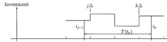
Fig. 1. Computing the scrapping time.
an integral on an interval whose endpoints are not integer multiples ofD, we have to be careful with the"rst and the last terms:
P
b aF(t) dt"(k
1D!a)F((k1!1/2)D)#DF((k1#1/2)D)#2
#DF((k
2!1/2)D)#(b!k2D)F((k2#1/2)D),
wherek1Dis the smallest integer multiple ofDwhich is larger or equal thana, and wherek
2Dis the largest integer multiple ofDwhich is smaller or equal than
b(see the discussion based on Fig. 1).
Finally, integrals of piecewise constant functions times exponential functions could be performed exactly, but we preferred to keep the midpoint rule, allowing for a small discrepancy, asDis small, and the exponential functions are slowly varying.3Hereafter we sett
k"(k#1/2)D, fork"0, 1,2,N, and we denote by
i
k and yk the values of investment and output at tk. Application of these principles leads to thediscrete-time problemanalog to (1)}(4):
max= $*4#"D
N + k/0
u(y
k!ik)exp(!otk), (6)
subject to
y
k"(jD!tk#¹(tk))ij~1#Dij#2#Dik~1#
D
2ik, k"0, 1,2,N, (7)
wherejDis the smallest integer multiple ofDlarger or equal thant
k!¹(tk), 1"(jD!t
k#¹(tk))ij~1e~ctj~1#Dije~ctj#2 #Di
k~1e~ctk~1#
D
2ike~ctk, k"0, 1,2,N, 04i
k4yk, k"0, 1,2,N. (8)
giveni
Table 1
Numerical solution by iterative methods of a class of vintage capital models The resolution algorithm
(a)Initialization
Choose an initial investment vectorI0"[i(0)0 ,i(0)1 ,2,i(0)
N]@and a stopping
parametere'0. Compute the induced scrapping time and output vectors,
¹0and>0, using (7) and (8).
(b)Maximization step by step(Gauss}Seidel step) Step 0. Solvei(1)
and the induced updated scrapping time and output vectors¹1and>1. (c)Gauss}Seidel iteration
Given a vector normD.D, ifDI1!I0D/DI0D(e, STOP and returnI0; else setI0equal toI1and go to steps (b) and (c).
A word of explanation on how (1)}(4) is discretized in (6)}(8). The computa-tion of (6) must be possible as soon as we get a set of values of a trial funccomputa-tioni, i.e., a set ofN#1 numbersi
0,i1,2,iN. To this end, we need the corresponding numbers y
0,y1,2,yN. These values of y are computed from (7) which is the exact value of the integral (2) at t
k, k"0, 1,2,N, as far as the functioni is assumed to be piecewise constant. As the lower boundt
k!¹(tk) is normally not an integer multiple of D, we have to consider the integer j such that (j!1)D(t
k!¹(tk)4jD. Fig. 1 makes it clear.
We see that the formula (7) represents indeed the sum of rectangular areas betweent
kandtk!¹(tk). Well, everything is all right provided¹(tk) is known. This one is now computed from (3), according to the same principles, assuming
i(z) exp(!cz) reasonably close to a piecewise constant function. The formula (8) is actually an equation for the unknown ¹(t
k)"¹k. We get the new area, advancing from right to left, summing the successive rectangular areas Di
kexp(!ctk)/2,Dik~1exp(!ctk~1),2up to the point where we get a number, sayalarger than one, by summing the last small rectangleDi
j~1exp(!ctj~1). This means that we went too far to the left (that is howjis found) by an amount
a!1. The left endpoint of the integral is therefore not (j!1)D, but
t
k!¹(tk)"(j!1)D#(a!1)/[ij~1exp(!ctj~1)], yielding the computed value of ¹(t
k). The maximization (6) is performed by iteration. At each iteration, we use a step-by-step maximization device. Precise-ly, at each step, we look at the in#uence of a single valuei
kassociated to a time
t
4Indeed, in our most re"ned tests, we tookD"0.1, about 1% of the average value of the scrapping time¹, and a time solution horizon equal to 100, about 10 times the average¹. So, we had about 103one-dimensional maximizations to perform per iteration. Finally, at least 100 iterations (c) are needed to locate the"xed-point for a convergence tolerance level around 10~4.
5As the popular steepest descent algorithm, see again Luenberger (1965, pp. 148}154). =
$*4# as a function of the sole investment vector ordinates,=$*4#(i0,i1,2,iN), since the output and scrapping time ordinates are computed from the invest-ment vector thanks to Eqs. (7) and (8). The whole algorithm works as reported in Table 1.
As one can see, we follow basically a Gauss}Seidel approach for the location of the optimal solution paths. At each Gauss}Seidel iteration, a step-by-step maximization is performed. At each step k of iterations (b), the discretized integral is maximized with respect to the ordinatei
k of the investment vector, keeping unchanged future investment ordinates i
k`1, ik`22, if any, with respect to the base, with the preceding investment ordinates i
l, 04l4k!1, updated thanks to the already performed maximization steps. However, even if we abstract away from the required optimization work, the implemented maximization device and the need to recomputeyand ¹values at each step makes the whole algorithm much more complex than the standard Gauss}Seidel scheme. Indeed, we have right now still no satisfactory hints on the behavior of the error through iterations (c).4
It should be noted, that except the required (and costly) updating ofyand ¹ at each maximization step, our steps (b) and (c) correspond to the cyclic coordinate descent optimization algorithm as described in Luenberger (1965, pp. 158}161), for unconstrained problems. This algorithm may be extremely appealing because of its easy implementation as it does not require any informa-tion on the gradient of the objective funcinforma-tions in contrast to most alternative optimization methods.5It follows that the cyclic descent algorithm can prove an excellent resolution technique when optimization has to be performed with respect to a very large number of choice variables as gradient information is extremely costly in this case. Since we are optimizing with respect to an investment vector, [i
0 i1 2iN]@, whenNis large, the cyclic descent algorithm appears very attractive for our purposes. Although this algorithm is known to have slower convergence rates than certain gradient-based optimization methods, we "nd it most useful in practice. This is in part due to certain theoretical properties of the models under considerations as explained in the next subsection.
3.2. Theoretical justixcations of the numerical setting
6Note that the sums appearing in (8) in Section 3.1 can be written as integrals as we are dealing with piecewise constant functions. This is done for convenience in this section.
a di!erential relation that shows clearly how and why the solutions provided by the algorithm are related to the optimality conditions of the original optimiza-tion problem.
Proposition. The discretized integral=
$*4#is a concave function,when considered as a function of a single ordinatei(t
0), for anyxxedt050. depends on all the changes induced in the various values c((j#1/2)D). Let
t
1"(j#1/2)D be another time abscissa. We havec(t1)"y(t1)!i(t1), so we have only to appreciate the change iny(t
1), which depends on¹(t1). From (8), subtract the&old'equation (8):
thanks to (9). We just got the increase of c(t
1)"y(t1)!i(t1), as far as
t
1!¹(t1)4t0(t1. Att0, the change is of course
c(t
0)b!c(t0)a"y(t0)!b![y(t0)!a]"a!b, and the change for=is
=(b)!=(a)
"D[u(c(t
0)a#a!b)!u(c(t0)a]e~ot0
#D +
t1~T(t1)yt0:t1
Mu(c(t
1)a
#(b!a)D[1!ec(t1~T(t1)~t0)])!u(c(t
1)a)Ne~ot1, (10)
forbclose to aand for smallD.
As (10) is a linear combination of concave functions of b, =(b) is indeed a concave function too, for b in a small interval, but concavity must only be established locally to hold everywhere. h
As=
$*4#is now known to be a concave function of a singleiordinate, we are therefore sure that=
$*4#(x) has a unique maximum in the admissible range, i.e., from x"0 up to the value such that x"i(t
0)"y(t0). Provided that all the di!erentiations are valid (or in other words that an interior solution exists for the optimization problem at t
0), an interesting consequence of (10) is the di!erential relation whenbPa"x:
=@
$*4#(x)"D
C
!u@(c(t0))e~ot0 #P
t0`J(t0)t0
u@(c(t
1))[1!ec(t1~T(t1)~t0)]e~ot1dt1
D
, (11) and=@4. An example
Let us solve the problem witho"0.05,c"0.03,u(c)"ch,h"0.85 close to 1. So we have a weakly concave function to maximize, and we expect rather a rough behavior of the solution paths. The balanced growth path solution is
i(t)"0.1078 exp(0.03t): if this law holds fort(0, it will still hold whent50. As one expects a perturbation of this law, one makes the computations with
i
k approximatingOne decides to takei(t) exp(i(t!)"c0.3 exp(0.03t) att"(k#t) on1/2)tD(, k0. This is much too high! At"0, 1,2
t"0, the economy is allowed to react. What will happen? Let us look at the record. One starts with trial values i(t)"0.1078 exp(0.03t) at t'0, i.e.,
i
k"0.1078 for all k50. Let us perform the approximate calculations with a (much too large) time stepD"1. The results of the step by step maximization for i
0, i1, i3 and i4 are reported in Table 2. First, we look at the discretized integral =
$*4# for several test values i0, keeping i1, i2, etc. unchanged. The discretized integral is the largest wheni
0"0, which is not surprising, asi(t) was too large att(0. We keepi
0"0, and makei1move. Again,i1"0 is best. And we get the same answer for i
2. Setting i0"i1"i2"0, we maximize with respect toi
3. Some change at last, the besti3appears to be close to 0.11. We now look ati
4. Here, the best value ofi4 is about 0.18.
One goes on with next values (in order not to be bothered by truncated series e!ects in the estimation of the integral, we took a big upper bound,N"500). These successive maximizations of =
$*4# (steps (b) using the terminology of Section 3.1) lead to the "rst approximation to i(t) exp(!ct). The job is not
"nished yet! We just performed maximization of =
$*4# on each ik, keeping unchanged thei
j's forj(k. This is only a limited way to see howik interacts with its neighbors, and we start again a whole run of maximizations following exactly the same principles as before (step (c) in the terminology of Section 3.1). Such a process is often called&relaxation', as it was"rst used in the calculation of complicated mechanical devices, with lots of interacting parts. The calculation considered only a limited number of links, ignoring (i.e.,relaxing) the other ones. Of course, when such a run of simpli"ed calculations was achieved for all parts, there was still no exact matching, and the whole process was restarted again, and again.
On our example, a second iteration (or a second run of maximizations) does not change the values of i
0,i1, and i2, which are still kept at the zero level. However, the best i
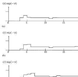
3 is found to be no more 0.11, but 0.04. Things hardly changed. After about 20 iterations, the"nal shape (at this poorD"1 precision) appears. Fig. 2 displays the patterns of (detrended) investment obtained after the "rst, the second, and the twentieth iteration of type (c).
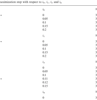
Table 2
Numerical solution by iterative methods of a class of vintage capital models, results of the"rst maximization step with respect toi
0,i1,i3andi4 i
0 =$*4#
P 0 32.7516401
0.05 32.7313349
0.1 32.7089774
0.15 32.6845603
0.2 32.6588714
i
1 =$*4#
P 0 32.778625
0.05 32.7673855
0.1 32.7539278
0.15 32.7379688
0.2 32.7206465
i
3 =$*4#
0 32.7801023
0.05 32.7851276
0.1 32.787636
P 0.11 32.7876691
0.12 32.7875742
0.15 32.786856
i
4 =$*4#
0 32.7758335
0.05 32.7825734
0.1 32.7873551
0.15 32.7884092
0.16 32.7884577
0.17 32.7884902
P 0.18 32.7885064
0.19 32.7884807
big (D"1), the obtained paths are not su$ciently&"ne', even after 20 iterations. Indeed, much more work (150 iterations withD"0.2) is needed for disclosing with"ner detail the solution. The obtained solution is reported in Fig. 3. The solution settles in a regime of slowly damped oscillations about the limit value of 0.1078 (indicated by a thin horizontal line in Fig. 3). We have also shown in dashed line the analytical solution of the (continuous) problem ath"1 accord-ing to Boucekkine et al. (1997a).
Fig. 2. (a) The investment pattern after one Gauss}Seidel iteration forD"1. (b) The investment pattern after 2 Gauss}Seidel iterations forD"1. (c) The investment pattern after 20 Gauss}Seidel iterations forD"1.
Fig. 3. The investment pattern after 150 Gauss}Seidel iterations forD"0.2.
7¹His indeed the"xed point of functionF(x)"!(1/c)¸n(1!o#c!c/o#(c/o) exp(!ox)). With c"0.03 and o"0.05, optimal scrapping ¹H is around 9. With the initial condition, i(t)"0.3 exp(0.03t),t(0, the constraint (3) of the optimization problem implies¹(0)(¹Hsince
¹(0) is around 3.3.
8Indeed, except the updating of state variables using the constraints of the considered optimiza-tion problem, which is model speci"c, the rest of the method is absolutely general.
corresponding to everlasting replacement echoes, as shown in the"gure above. Whenh"0.85, the economy starts investing before and oscillations are dam-ped: This is obviously due to consumption smoothing when utility functions are strictly concave. Much smoother solution paths can be obtained for lowerh's values, but we have preferred a parameterization close to the linear utility case and initial conditions very far from the corresponding balanced growth paths so as to illustrate the ability of our method to reproduce (highly) irregular solution paths.
5. Concluding remarks
In this paper, we have built up a Gauss}Seidel scheme in order to solve vintage capital models, especially those with Leontie! technologies. Using theoretical and experimental arguments, we have shown why our approach is suitable to deal with this class of models. In particular, the use of a cyclic coordinate descent optimization technique within our procedure seems adapted to circumvent the extremely arduous problems coming from the com-plex structure of the optimality conditions of these models. It should be noted that our method is quite general, and can be applied to a much larger set of dynamic models than those referenced in this paper.8 Furthermore, there is room for many potential improvements and adaptations of the method depending on the concrete problem under consideration. We have just presented a basic algorithmic scheme, which is #exible to a large extent. Clearly, the simple numerical integration technique we have adopted for convenience in this paper can be replaced by a more complex and accurate method. Also, the elementary relaxation scheme we have implemented so far can be replaced by more e$cient "rst-order iterations like successive over relaxation (SOR) processes. Practitioners can take advantage of this#exibility to optimize their numerical setting if necessary. This is indeed a major strength of our method.
References
Aghion, Ph., Howitt, P., 1994. Growth and unemployment. Review of Economic Studies 61, 477}494.
Benhabib, J., Rustichini, A., 1993. A vintage capital model of investment and growth. In: Becker, R. et al. (Eds.), General Equilibrium, Growth and Trade. II The Legacy of Lionel McKenzie. Academic Press, New York, 248}301.
Boucekkine, R., Germain, M., Licandro, O., 1997a. Replacement echoes in the vintage capital growth models. Journal of Economic Theory 74, 333}348.
Boucekkine, R., Licandro, O., Paul, C., 1997b. Di!erential-di!erence equations in economics: on the numerical solution of vintage capital growth models. Journal of Economic Dynamics and Control 21, 347}362.
Boucekkine, R., Germain, M., Licandro, O., Magnus, A., 1998. Creative destruction, investment volatility and the average age of capital. Journal of Economic Growth 3, 361}384.
Boucekkine, R., del RmHo, F., Licandro, O., 1999. Endogenous Vs exogenously driven#uctuations in vintage capital models. Journal of Economic Theory 88, 161}187.
Caballero, R., Hammour, M., 1996. On the timing and e$ciency of creative destruction. Quarterly Journal of Economics 111, 805}851.
Caballero, R., Hammour, M., 1998. Jobless growth: appropriability, factor substitution, and unem-ployment. Carnegie}Rochester Conference Series on Public Policy 48, 51}94.
Judd, K., 1998. Numerical Methods in Economics. The MIT Press, Cambridge, MA.