www.elsevier.com/locate/spa
Polling systems in the critical regime
Mikhail Menshikov
a;1, Sergei Zuyev
b;∗;2aDepartment of Mathematical Sciences, University of Durham, Old Shire Hall, Durham,
DH1 3HP, UK
bDepartment of Statistics and Modelling Science, University of Strathclyde, 26Richmond Street,
Glasgow, G1 1XH, Scotland, UK
Received 12 April 2000; received in revised form 17 October 2000; accepted 24 October 2000
Abstract
We study polling systems with Poisson arrival streams and exhaustive service discipline in the critical load case=1. We show that the system may exhibit null-recurrence or transient behavior and give the corresponding conditions in terms of the rst two moments of the distribution of service and switching times. For models with two nodes we establish existence of moments of small orders for the return time to the origin of the corresponding embedded Markov chain in the case of null-recurrence. c 2001 Elsevier Science B.V. All rights reserved.
MSC:Primary: 60G20; 68M20; Secondary: 90B22
Keywords:Polling systems; Greedy server; Transience; Null-recurrence; Lyapunov functions; Markov walk
1. Introduction
Consider the following queuing model. Customers arrive at two nodes 1 and 2 with innite buers according to independent homogeneous Poisson processes with rates1 and2, respectively. A single server visits (polls) the nodes performing the service of the customers accumulated there. The service times of the customers at nodei(i=1;2) is a sequence of i.i.d. random variables each distributed as a variablei with the mean
mi. The service times are assumed to be independent of the system’s state. The served
customers leave the system. After the server has started service at nodei it continues there until the buer is empty (this is the so-called exhaustive service discipline). Then the server leaves the i1th node and moves to the other node i2. The switching time between nodes i1 and i2 is a random variable ri1i2 independent of the number
of customers present in the system. For many types of polling systems the exhaustive
∗Corresponding author.
E-mail addresses:[email protected] (M. Menshikov), [email protected] (S. Zuyev).
1www.maths.dur.ac.uk=stats=people=mm=mm.html 2www.stams.strath.ac.uk=∼sergei
discipline is known to minimize the main performance characteristics, such as the number of customers waiting in a queue and the total amount of unnished work (Liu et al. 1992).
The stability of the system largely depends on the load rate parameter
=1m1+2m2: (1)
In more general settings than the one considered here it was proved that the system is ergodic if and only if ¡1 (Foss and Last, 1996). In this paper we concentrate on the critical case, hardly studied in the literature, where
1m1+2m2= 1: (2)
Thus in the long run the mean number of customers coming to the system equals the mean number of the served customers. We show that in this critical regime the system may exhibit two dierent kinds of behavior: null-recurrence or transience depending on interrelation between the rst two moments of the switching and the service times. The importance for stability of the mean switching time has already been recognized for systems with switching policies other than exhaustive when ¡1 (see, e.g. Borovkov and Schassberger, 1994 and Foss and Chernova, 1996 and the references therein).
The main approach to study stability properties of a Markov chain’s trajectories is the technique of Lyapunov functions. The Foster-type criteria for countable Markov chains employ quantities of the type
E[f(Xt+1)−f(Xt)|f(Xt) =u]: (3)
In many models, including the polling models we consider in this paper, the quantity above behaves like O(u−1) while the second moment of the variable f(X
t+1)−f(Xt)
has an order of a constant asu grows. The result of Lamperti (see Theorem 1 below) shows that in this case the chain’s asymptotic behavior is determined by the rst two moments of that variable. The Lyapunov function f that we construct behaves asymptotically linearly as the number of the customers in the system grows. Some account for the switching needs, however, to be taken to insure that the corresponding relation between the moments holds for all system states.
The aim of the paper, as the authors see it, is not to obtain the asymptotic behav-ior results for the widest possible class of polling systems in the critical regime, but rather to demonstrate the technique that we believe, can be successfully applied in other similar situations. For instance, the results of this paper immediately generalize to the case when the customers arrive at each node in batches with independent identi-cally distributed sizes. Here, we have intentionally avoided generalizations that would over-complicate sometimes already quite technical proofs.
The structure of the paper is the following. Section 2 characterizes the null-recurrence and the transience regions under condition (2) for the polling system with two nodes described earlier.
In Section 4 we consider systems with more than 2 nodes under critical load. We establish bounds for transience and null-recurrence when the switching discipline is close to the greedy-type policy in that the server never switches to the least loaded nodes.
Finally, for convenience of the reader, we give in the appendix formulations of other theorems that we use in our proofs.
2. Polling systems with two nodes: transience and recurrence
In this section we study the polling system with 2 nodes described above. As in the case of M|GI|1 queue, the evolution of the system is completely determined by an embedded Markov chain Xt with discrete time t describing the state of the system at
the epochs of the service completion of customers and at the epochs of the switching completion. The phase space of the chain Xt is a pair of quadrants Z2+× {1;2}: in state (n1; n2;1) with n1¿1 the server is in the node 1 just after the departure of a served customer and there are stilln1 customers at node 1 andn2 customers at node 2. In state (0; n2;1) the server has just nished service of the last customer in node 1, started switching to node 2 and there are n2 customers waiting in the buer 2 at the time instant when it leaves node 1. States (n1; n2;2), when the server is in node 2, have similar meaning.
For the critical regime we deal with in this paper, we make extensive use of the following variant of Lamperti’s result (cf. Theorem 3:2 in Lamperti, 1960):
Theorem 1. LetXt be a time-homogeneous Markov chain on a countable phase space
A={n}.Assume that there exists a positive functionf:A→R+ with the following properties:
lim
n→∞f(n) = +∞ (4) and there exist constants C0; ¿0 such that
E[|f(Xt+1)−f(Xt)|2+|Xt=n]6C0 for all n: (5)
Denote
an=f(n)·E[f(Xt+1)−f(Xt)|Xt=n];
bn=E[(f(Xt+1)−f(Xt))2|Xt=n]:
Then Xt is recurrent if lim sup(2an −bn)¡0; and Xt is transient if lim inf (2an−
bn)¿0.
Proof. To conform with Lamperti’s notation, denote xn=f(n); (xn) =an=xn. Then
lim sup(2an−bn)¡0 implies that for some ¿0 one has 2xn(xn)−bn¡− for
all suciently large n. Thus (xn)¡ bn=(2xn), condition (3:13) of Lamperti (1960,
Theorem 3:2) is veried implying that Xt is recurrent.
If, in contrast, lim inf (2an−bn)¿0, then 2xn(xn)−bn¿ and thus (xn)¿(1 +
inequalitybn6C02=(2+) for all n. Therefore(xn)¿ bn=(2xn) with= (1+C0−2=(2+))
¿1, condition (3:14) of Lamperti (1960, Theorem 3:2) is valid so thatXt is transient.
Corollary 1. Assume there exist limitsliman=a and limbn=b.Then Xt is recurrent
if 2a ¡ b and Xt is transient if 2a ¿ b.
Our principal result for the polling model with 2 nodes is given by the following theorem.
Theorem 2. Assume there exists ¿0 such that
E2+
Then under Condition (2) the system is null-recurrent if (i)
R ¡ L ; (8)
and it is transient if (ii)
R ¿ L : (9)
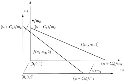
Proof. First, we give the description of the functionfemployed in Theorem 1, dened on the phase space Z2 For any positiveu the corresponding contour of the functionF is the line
m1x1
u+A1
+ m2x2
u+A2
= 1: (11)
It is straightforward to verify that
Fig. 1. The contours at leveluof the functionf.
The asymptotic behavior of the function F(x1; x2) =F(x1; x2; A1; A2) is of the main importance for us. We have F(x1; x2)=V(x1; x2)→1 as x1+x2 → ∞. For any xed non-negative constantC and for any k1; k2¿−C, one has
@2F @xi@xj
(x1+k1; x2+k2)
6O
x1+x2+k1+k2
V3(x
1−C; x2−C)
= O
x1+x2+k1+k2
F3(x 1; x2)
(12)
as x1+x2→ ∞. Therefore for k= (k1; k2)T we have the following development:
F(x1+k1; x2+k2)−F(x1; x2) =∇F(x1; x2)·k+D2F(x1+1k1; x2+2k2)k·k
=F(x1; x2)
V(x1; x2)
(m1k1+m2k2) +
A2m1k1+A1m2k2
V(x1; x2)
+O
x1+x2+k1+k2
F3(x 1; x2)
: (13)
The explicit form of O-term above as a function of 1; 2 can be written down from the expressions above for the second derivatives ofF.
Now let us dene the functionf as follows:
f(n1; n2;1) =F(n1; n2; C0;−C1);
f(n1; n2;2) =F(n1; n2;−C3; C2)
(14)
(see Fig. 1), where the parameters C0; C1; C2; C3 will be specied later to provide the validity of the conditions of Theorem 1. Such a choice of the function f can be informally explained as follows.
In the case when the switching time between the nodes is zero, the direct compu-tation of the quantity (3) shows that a linear function f(x1; x2; i) =m1x1+m2x2 is a martingale, from where the null-recurrence of the embedded Markov chain Xt can be
order O(1) on the axes corresponding to the customers coming to the system during the switching of the server. Given a large f(Xt) =u=m1x1+m2x2, the share of time the chain spends on switching has order O(u−1). Intuitively, the drift dened in (3) has the same order and that is how Lamperti’s technique for systems with asymptotically small drift comes into play. Formally, to cope with jumps on the axes, we slightly change the function f as shown on Fig. 1. This results in a drift of order O(u−1) appearing inside the quadrants which is controlled by the constants C0; : : : ; C3. Note also that if the share of time spent on switching is not asymptotically small asu grows (as is the case, for instance, for thegatedservice discipline) the above argument does not hold anymore. Based on Theorem 1, we might suggest that such systems exhibit a transience behavior under the critical load, although a formal analysis is, of course, necessary in each case.
Letij be a random variable distributed as the number of customers arriving at node
j during the service time of a customer in node i. This distribution does not depend on the number of customers in the system. If the server is in node 1 and the state when it started the last service was (n1; n2;1) with n1¿1 then by (13) we have
E[f(Xt+1)−f(Xt)|Xt= (n1; n2;1)] =E[f(n1+11−1; n2+12;1)−f(n1; n2;1)]
= f(n1; n2;1)
V(n1; n2; C0;−C1)
E[m1(11−1) +m212]
+−m1C1(E11−1) +m2C0E12
V(n1; n2; C0;−C1)
+ O
n1+n2
f3(n 1; n2;1)
(15)
(−1 here accounts for the customer that has just been served in the node 1.) Since Eij=EE[ij|i] =Eji=jmi, then by (2) we have E[m1(11−1) +m212] = 0. Therefore, taking into consideration that (n1+n2)=f2(n1; n2;1) vanishes, we obtain that
a(n1; n2;1)=f(n1; n2;1)E[f(Xt+1)−f(Xt)|Xt= (n1; n2;1)]
=−m1C1(E11−1) +m2C0E12+ o(1) (16)
as n1+n2→ ∞. Furthermore, Expression (15) also yields
b(n1; n2;1)=E[(f(Xt+1)−f(Xt))
2|X
t= (n1; n2;1)]
= f 2(n
1; n2;1)
V2(n
1; n2; C0;−C1)
E(m1(11−1) +m212)2+ o(1)
=E[m1(11−1) +m212]2+ o(1): (17)
Similarly, if the server is in node 2 andn2¿1 then
a(n1; n2;2)=f(n1; n2;2)E[f(Xt+1)−f(Xt)|Xt= (n1; n2;2)]
=f(n1; n2;2)E[f(n1+21; n2+22−1;2)−f(n1; n2;2)]
and
b(n1; n2;2)=E[(f(Xt+1)−f(Xt))
2|X
t= (n1; n2;2)]
=E[m121+m2(22−1)]2+ o(1): (19)
Consider now the case when the server switches between the nodes. Denote by ij
the number of customers arriving at node j while the server switches from node i to the other one and let i= (i1; i2)T. Obviously E
1j=jEr12 and E2j=jEr21. Therefore, using (13) again and (2) we obtain that
E[f(Xt+1)−f(Xt)|Xt= (0; n2;1)] =Ef(11; n2+12;2)−f(0; n2;1)
=f(0; n2;2)−f(0; n2;1) +∇f(0; n2;2)·E 1+ O
n2
f3(0; n 2;2)
=−(C1+C2) +
m1m2n2
m2n2−C2−C3
E11+m2E12+ O(n−22 )
=−(C1+C2) +m11Er12+m22Er12+1Er12
m1(C2+C3)
m2n2−C2−C3
+ O(n−22 )
=−(C1+C2) +Er12+1Er12
m1(C2+C3)
m2n2−C2−C3
+ O(n−22 ) (20)
and
E[f(Xt+1)−f(Xt)|Xt= (n1;0;2)] =Ef(n1+21; 22;1)−f(n1;0;2)
=f(n1;0;1)−f(n1;0;2) +∇f(n1;0;1)·E 2+ O
n1
f3(n 1;0;1)
=−(C0+C3) +m1E21+
m1m2n1
m1n1−C0−C1
E22+ O(n−2 1 )
=−(C0+C3) +Er21+2Er21
m2(C0+C1)
m1n1−C0−C1
+ O(n−21 ): (21)
To obtain expressions for the second moments of the Lyapunov function’s increment for the boundary states, it is sucient to note that
f(Xt+1)−f(Xt) =−(C1+C2) +m111+m212+ o(1) given Xt= (0; n2;1);
f(Xt+1)−f(Xt) =−(C0+C3) +m121+m222+ o(1) given Xt= (n1;0;2) (compare with the third line of (20) and of (21), respectively). Therefore the second moments are nite and equal, respectively, to
b(0; n2;1)=E[m111+m212−(C1+C2)]
2+ o(1)
; (22)
b(n1;0;2)=E[m121+m222−(C0+C3)]
2+ o(1): (23)
Denition (10) of the functionF yields that
1
for all suciently largen1+n2. From (13) and Lemma 1 (see the appendix) it is readily seen that the existence of (2 +)-moments of the variables ij and ij is ensured by
the validity of condition (6). Thus condition (5) of Theorem 1 is also satised. Next, in view of (16) – (21), the condition lim sup(2an−bn)¡0 of Theorem 1 is
satised for all suciently large n1+n2 if
m1C1(1−E11) +m2C0E12¡12E[m1(11−1) +m212]2 def=12B1;
m1C2E21+m2C3(1−E22)¡12E[m121+m2(22−1)]2 def=12B2;
Er12¡ C1+C2;
Er21¡ C0+C3: (25)
The rst inequality above is relevant for statesn= (n1; n2;1) with n1¿1, the second is relevant for n= (n1; n2;2) with n2¿1, the third and the last equations guarantee that an → −∞when n runs to innity along the boundaries (0; n2;1) and (n1;0;2).
Introducing the positive parameters from the last two inequalities
1=C1+C2−Er12¿0;
2=C0+C3−Er21¿0;
we see that the rst two inequalities in (25) are equivalent to
C0+C1¡
B1 2m1m22
;
C0+C1¿E[r12+r21]−
B2 2m1m21
+1+2:
(26)
Therefore if
R=E[r12+r21]¡
1B1+2B2 212m1m2
(27)
holds, there exist 1¿0; 2¿0; C0 and C1 (and thus C0; C1; C2; C3) such that all inequalities (25) are met and the chain is recurrent by Theorem 1. It is easy to obtain that
Ekj2 =jmk+2jE2k;
Ekikj=ijE2k if i=j: (28)
Therefore, making use of Kronecker’s symbol jk that is 0 unless j=k when it is 1,
we may write
Bk=E
j
mj(kj−kj) 2
=
i; j
mimjE(ki−ki)(kj−kj)
=
i; j
mimjEkikj−
i
mkmiEki−
j
=
i=j
mimjijE2k+
j
m2j(jmk+j2E2k)−2m2k
j
jmj+m2k
=E2
k
j
jmj
2 +mk
j
m2jj−m2k= vark+mk
j
m2jj: (29)
Finally, substituting this expression into (27) and again using the fact that
jjmj=1,
reduces the latter to (8).
As was shown in Foss and Last (1996) the case when the workload 1m1+2m2 equals 1 is non-ergodic so the recurrence here is, in fact, null-recurrence. In the next section, we will study the moments of small orders for the return time to a neighbor-hood of the origin.
Similarly, the condition lim inf (2an−bn)¿0 of Theorem 1 will be satised if (25)
holds with “¡” replaced with “¿” everywhere. Proceeding as above (that basically means changing all the inequalities to the opposite ones) we nd that a choice of
1¿0; 2¿0; C0 and C2 for this new system exists if
E[r12+r21]¿
lB1+2B2 212m1m2
or, equivalently, (9) holds, so that the chain is now transient by Theorem 1.
In particular, for symmetric systems with exponentially distributed service times we have 1=2def=, m1=m2= 1=(2); E2i = 1=(22) and r12=r21def=r. Thus we have the following corollary:
Corollary 2. A symmetric system with exponentially distributed service times is null-recurrent ifEr ¡1= and transient if Er ¿1=.
3. Existence of moments of hitting times
In this section we study the existence of small order moments of the rst-hitting time of compact subsets for the embedded Markov chain Xt described in Section 2.
Given a compact set of the state space, the rst-hitting time is dened as follows:
(u0) = inf{t:X0=u0;Xt ∈}:
The main result of this section is the following theorem.
Theorem 3. Assume the conditions of Theorem 2 are satised and that R ¡ L. Let
N ={(n1; n2; i)∈Z2+× {1;2}:n1+n26N}:
Then for all suciently large N and all but nite number of starting states X0= (n1; n2; i) one has
(i) for all p ¿1
(ii) for allp ¡12(1−R=L)there existsN such that for any starting state u0 one has Ep
N(u0)¡∞.Moreover; for any p
′¡ p ¡1
2(1−R=L) there exists a constant
C(p′; p) such that
Ep′
N(u0)¡ C(p ′; p)(m
1n1+m2n2)2p (30) for all starting states u0= (n1; n2; i).
Proof. We start with proving Part (ii) by checking that the conditions of Theorem 5 are satised for the processXt.
Letf be the same as in the proof of Theorem 2 (see (14)). From the bounds (24) it follows that for any suciently large N there exists A proportional to N such that
N contains compact
KA={(n1; n2; j):f(n1; n2; j)6A}:
Since N(u0)6KA(u0) then it is sucient to prove (ii) for KA(u0).
Assume that Xt=n and denote un=f(n), ’n=f(Xt+1)−f(Xt). Then for all
p ¿0 one has the following Taylor’s expansion:
f2p(Xt+1)−f2p(Xt) = (un+’n)2p−u2np
=pu2np−2(2un’n+ (2p−1)’2n) +Rn; (31)
where the residual term Rn is given by
p(2p−1)(2p−2)’3n 1
0
(un+’n)2p−3(1−)2d:
Next, for as in Theorem 2 uniformly for all large n one has
E[|’n|2+|Xt=n]6C ¡∞ (32) since by (24) the (2+)-moment of’n is bounded by a constant times the
correspond-ing moments of the variablesij or ij that were introduced in the proof of Theorem 2
and represent the number of arrivals during a typical service or switching time. Rela-tion (32) guarantees applicability of Lemma 10 from Aspandiiarov et al. (1996) due to which for any ¿0 there exists A such that for all n ∈KA one has
E[|Rn| |Xt=n]6u2np−2=2:
Inequality (A.4) will, therefore, be satised withYt=f(Xt) for all suciently largeA
(and thus,N) and all n ∈KA if
2unE’n+ (2p−1)E’2n¡−
2p: (33)
Exactly the same way we did it in the proof of Theorem 2, we write the last condition in the cases when the staten corresponds to the service in node 1, 2 or to the switching
between the nodes and arrive at the following system similar to (25):
m1C1(1−E11) +m2C0E12¡−
4p+ (1−2p)B1=2;
m1C2E21+m2C3(1−E22)¡−
Er12−(C1+C2)¡0;
Er21−(C0+C3)¡0: (34)
Recall that the last two inequalities imply that unE’n→ −∞ when n runs along the
boundaries (0; n2;1) and n= (n1;0;2) that is sucient for (33) to hold for these n.
Sincecan be chosen arbitrarily small, this system is, in fact, equivalent to the system (25) withB1; B2 replaced with (1−2p)B1; (1−2p)B2, respectively. And similarly, a choice of C0; C1; C2 and C3 is possible whenever
R=E[r12+r21]¡1−2p 2m1m2
(B1=2+B2=1) = (1−2p)L
(compare with (27)). Now Theorem 5 applies implying niteness of the p-moment of KA(u0) and thus N(u0) for all u0 and all suciently large N. Finally, given
p′¡ p ¡1
2(1−R=L) in view of (24) estimate (30) simply follows from (A.5). The proof of Part (i) of the theorem is based on Theorem 6. ChooseA= O(N) here such that the compact
KA={(n1; n2; j):f(n1; n2; j)6A}
contains the compactN. Obviously, if a moment of the return time toKA is innite,
so is the case for any of its subset .
Let the process Yt be the same as above except that the constants C0; : : : ; C3 are chosen in order to have the opposite inequalities in (34). Such a choice exists whenever
R ¿(1−2p)L, that will yield inequality (A.11).
In order to satisfy the other conditions of Theorem 6 we need to construct the dominating processZt. Let
˜
f(n1; n2;1) =F(2n1;2n2;C˜0;−C˜1);
˜
f(n1; n2;2) =F(2n1;2n2;−C˜3;C˜2) (35)
with some constants ˜C0; : : : ;C˜3 to be identied later and deneZt to be ˜f(Xt) (compare
with (14)).
Since ˜f(n1; n2; i)∼2f(n1; n2; i)∼2(m1n1+m2n2) as n1+n2 → ∞, the conditions (A.6) – (A.8) are satised for all suciently largeAwith B= 1 whatever is the choice of the constants C0; : : : ; C3 and ˜C0; : : : ;C˜3. Condition (A.9) is satised by
m1x1+m2x2¡f˜(x1; x2; i)¡4(m1x1+m2x2)
and niteness of the second moments of the variables ij and ij.
Finally, in order to check (A.10), rewrite (31) with un= ˜f(n), ’n= ˜f(Xt+1)−
˜
f(Xt) and ˜f; r in place of f; p, respectively. Estimating the residual term exactly
the same way as in (32), we see that (A.10) is satised for all suciently large A
if G= 2unE’n+ (2r−1)E’2n as in (33) is bounded. The developments (15) – (19)
for ˜f∼2f that simply manifests in changing ni to 2ni in the above formulas, imply
(0; n2;1) and (n1;0;2) if we choose the parameters ˜C0; : : : ;C˜3 so that to have Er12−( ˜C1+ ˜C2) = 0;
Er21−( ˜C0+ ˜C3) = 0:
The second term is bounded by (20), (21) and thus Condition (A.10) is satised for the process Zt with that choice of ˜C0; : : : ;C˜3.
Theorem 6 now applies foru0 ∈KA thus completing the proof of the theorem.
4. Systems with many nodes
In this section we study polling systems with N¿3 nodes. As before, the arrival streams are independent Poisson with ratei to node i= 1; : : : ; N, the service times are
independent with mean mi. We assume that as soon as the server starts service at a
nodekit does not leave it until the queue is empty. When there are no more customers in the node k, the server chooses the next node to switch to depending on the current state of the system. The switching time between nodeskandjisrkj. As in the previous
section, the evolution of the system can be described by a discrete Markov random walk
Xt in the space of vectors (n1; : : : ; nN;k)∈ZN+× {1; : : : ; N}, where ni is the number of
customers in nodei at the epochs of completion of the service andk is the node where the service is currently performed. The switching discipline is a rule that is applied when Xt visits the boundary states k= (n1; : : : ; nk−1;0; nk+1; : : : ; nN;k). Formally, it is
represented as a (possibly random) functionJ(k)→ {1; : : : ; N} \ {k}; k= 1; : : : ; N that
is called independently for each boundary statek.
The next theorem gives sucient conditions for null-recurrence and transience of the system in which the server, loosely speaking, never switches to the least loaded nodes. For instance, the systems with the greedy policy when the server switches to the node with the maximal number of customers, satisfy the condition (37) below with
= minimi=(Nmaximi). In contrast with the 2-node case, we are unable to characterize
explicitly the surface separating transient behavior from null-recurrence which is heavily dependent on the routing discipline. It is easily seen, however, that the gap between the bounds we give is minimal for symmetric systems with the greedy switching policy.
Theorem 4. Assume there exist ¿0 such that
E2+
i ¡∞ and Erij2+¡∞ (36)
for i; j= 1; : : : ; j and that the switching discipline possesses the following property: there exists0¡ ¡1 such that
P{J(n1; : : : ; nk−1;0; nk+1; : : : ; nN;k) =i}= 0 for all i such that mini
jmjnj
¡ :
(37)
Then under condition
N
j=1
the system is null-recurrent if
An expression for Bk is given by (29).
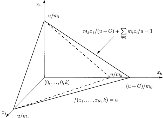
Proof. The proof is very similar to that of Theorem 2. We therefore omit identical details. The main tool is the construction of the Lyapunov functionf for the chain Xt
on the state spaceZN+× {1; : : : ; N}. Put
andC is a constant to be specied later. The contours at level u of this function are the planes
with the same function F used in the proof of Theorem 2 and dened in (10), then we have
wherejk is 0 ifj=k and 1, otherwise. And exploiting again the asymptotic properties
of the function F it can be similarly shown that
@2f
Fig. 2. The surfaces of levelu of the Lyapunov function f. The hyper-plane containing the mean drift vectors is dashed.
typical service time of a customer at a nodek. From (41) similarly to (15) we have
E[f(Xt+1)−f(Xt)|Xt= (n1; : : : ; nN;k)]
=E[fk(n1+k1; : : : ; nk+kk−1; : : : ; nN+kN)−fk(n1; : : : ; nN)]
=fk(n1; : : : ; nN)
Vk(n1; : : : ; nN)
E
mk(kk −1) +
j=k
mjkj
+ C
Vk(n1; : : : ; nN)
j=k
mjEkj+ O
jnj
f3
k(n1; : : : ; nN)
:
Therefore, noting that fk=Vk→1 asjnj→ ∞ and that by (38) we have
E
mk(kk−1) +
j=k
mjkj
=mk
kmk−1 +
j=k
jmj
= 0;
we obtain that
a(n1;:::; nN;k) def
=fk(n1; : : : ; nN)E[f(Xt+1)−f(Xt)|Xt= (n1; : : : ; nN;k)]
=Cmk
j=k
and
Consider now the case when the server switches between nodes. Denote by ki the
event i=J(n1; : : : ; nk−1;0; nk+1; : : : ; nN). Also denote by j(k; i) the random variable
distributed as the number of customers arrived to node j during the switching time
rki; (k; i) = (1(k; i); : : : ; N(k; i))⊤ and S=jmjnj. We then have
Taking into account that fi=Vi →1 as S → ∞, the above expression under condition
(38) becomes
−Cmini
S+C +Erki+ O((mini)
2S−3) + o(1):
According to our assumptions on the switching discipline we always have6mini=S61.
Therefore, if−C+ miniErki¿0 there exists a small positive 1 such that
E[f(Xt+1)−f(Xt)|Xt= (n1; : : : ; nk−1;0; nk+1; : : : ; nN;k)]¿1
providedS is large enough. Since the (2 +)-moment of the variable under expectation is nite by assumption (36), then the condition 2an−bn¿0 of Theorem 1 will be
satised for allsuciently distant boundary states if
−C+ min
i; k
Erki¿0: (44)
In view of (42) and (43) this condition will be satised for non-boundary states if
Cmk(1−kmk)¿
Conversely, if−C+ maxi; kErki¡0 then there exists a positive 2 such that
E[f(Xt+1)−f(Xt)|Xt= (n1; : : : ; nk−1;0; nk+1; : : : ; nN;k)]6−2
for all boundary states (n1; : : : ; nk−1;0; nk+1; : : : ; nN;k) with S=jmjnj large enough,
implying that 2an−bn¡0 for these states. If, in addition, the inequality opposite to
(45) holds, then 2an−bn¡0 also holds for all but nite number of states. The choice
of suchC is possible if (39) is satised and Xt is recurrent by Theorem 1.
The theorem is completely proved.
Acknowledgements
The authors are grateful to Serguei Foss for useful discussions, to Iain MacPhee and anonymous referees for thorough reading of the paper and their remarks.
Appendix
In the appendix we give the auxiliary results that we used in the proofs. The following fact was used in the proof of Theorem 2.
Lemma A.1. Let be a homogeneous Poisson point process on R with intensity
and be a positive random variable independent of . Let be the random variable equal to the numbers of points of in a random interval of length.Then E2+¡∞ implies E2+¡∞ for any0¡ ¡2.
Proof. Let ’(t) be the characteristic function of the variable. According to
Rama-chandran (1969, Theorem 5b) the existence of its 2 + moment is equivalent to convergence of the integral
It is straightforward to obtain that the characteristic function ’ of the variable is
written as’(t) =’(−i(eit−1)). Dierentiation with respect to t gives
LetYt; Zt be two discrete-time stochastic processes adapted to a ltration {Ft} and
taking values in an unbounded subset ofR+. The next two theorems proved in Lamperti (1960, Theorems 1 and 2, respectively) concern the moments of the rst-hitting times dened as
A(y) = inf{t:Yt6A; Y0=y}: (A.3)
Theorem A.1. Assume there exist ¿0; p ¿0such that for any t; Yt2p is integrable
and
Yt2−2pE[Yt2+1p −Yt2p|Ft]6− on{A(y)¿ t}: (A.4)
Then for any positive p′¡ p there exists a positive constant C=C(; p′; p) such that for ally¿0 one has
Ep′
A(y)6Cy
2p: (A.5)
We give the last theorem in a slightly dierent form than in Lamperti (1960). In the original paper the theorem was formulated for process Zt. It is sucient to
in-spect the proof of Theorem 2 there to see that, in fact, the following statement holds for Yt.
Theorem A.2. Assume there exist positive constantsr ¿1; A; B; C and Dsuch that
Z0¿ A; (A.6)
AB ¡ Y0=y6BZ0; (A.7)
∀t¿0; Yt6BZt; (A.8)
and on event {t ¡ A} one has
E[Zt2+1−Zt2|Ft]¿−C; (A.9)
Zt2−2rE[Zt2+1r −Zt2r|Ft]6D: (A.10)
If; in addition;for some positivepon{t ¡ AB(y)} the processYt2p is sub-martingale;
i.e.
E[Y2p
t+1−Y 2p
t |Ft]¿0; (A.11)
then for any p′¿ p; the moment Ep′
A (y) is innite.
References
Aspandiiarov, S., Iasnogorodski, R., Menshikov, M., 1996. Passage-time moments for nonnegative stochastic processes and an application to reected random walks in a quadrant. Ann. Probab. 24, 932–960.
Borovkov, A., Schassberger, R., 1994. Ergodicity of a polling network. Stochastic Process Appl. 50 (2), 253–262.
Foss, S., Last, G., 1996. Stability of polling systems with exhaustive service policies and state-dependent routing. Ann. Appl. Probab. 6, 116–137.
Lamperti, J., 1960. Criteria for the recurrence and transience of stochastic processes I. J. Math. Anal. Appl. 1, 314–330.