Understanding Educational Outcomes
of Students from Low-Income
Families
Evidence from a Liberal Arts College with a
Full Tuition Subsidy Program
Ralph Stinebrickner
Todd R. Stinebrickner
a b s t r a c t
Issues related to schooling attainment of children from low-income fami-lies arise frequently in current education policy debates. There has been a specific interest in understanding why a very high percentage of children from low-income families do not graduate from college and why the col-lege graduation rates of children from low-income families are substan-tially lower than those of children from other families. Using unique new data obtained directly from a high-quality liberal arts college that main-tains a full tuition subsidy program (and large room and board subsidies) for all students, this paper provides direct evidence that reasons unrelated to the direct costs of college are very important in explaining these realities.
I. Introduction
Issues related to the schooling attainment of children from low-in-come families arise frequently in current education policy debates. Although these issues span the entire spectrum of schooling levels, a recent increase in the relative wages of college graduates has contributed to a particular interest in understanding
Ralph Stinebrickner is a professor of mathematics at Berea College. Todd R. Stinebrickner is a profes-sor of economics at the University of Western Ontario. The authors would like to thank Pam Thomas for her invaluable assistance with this project, particularly the data extraction phase. They are also grateful for helpful comments which were provided by John Bound, Caroline M. Hoxby, Jeff Smith, Dan Black, Chris Swann, Ben Scafidi, Sarah Turner, Susan Dynarski, Scott Drewianka, and numerous seminar participants. The authors are grateful for generous funding from the Mellon Foundation and SSHRC. Ralph was supported in part by Berea College through funding for a sabbatical leave. Todd received generous support from the CIBC and the Agnes Cole Dark fund. Many useful discussions took place at the Osceola Research Institute. The data used in this article can be obtained from the author beginning February 2004 through January 2007.
[Submitted May 2001; accepted February 2002]
ISSN 022-166X2003 by the Board of Regents of the University of Wisconsin System
two interrelated facts associated with college attainment.1First, a very high
percent-age of the children from low-income families who graduate from high school do not graduate from college. Second, among high school graduates, the percentage of children from low-income families who graduate from college is substantially lower than the percentage of children from other families who graduate from college. Man-ski (1992) documents these facts using respondents from the High School and Be-yond (HS&B) who were high school seniors in 1980. He finds that five and one-half years after high school graduation only 0.11 of respondents from families in the lowest income quintile had graduated from four-year colleges, whereas 0.24 of respondents from families in the middle income quintile and 0.39 of respondents from families in the highest income quintile had graduated.
In order to graduate from college, a person must first make the decision to enter college and then must persist in college until graduation. Although much previous literature has specifically examined the college entrance decision, work such as Man-ski and Wise (1983), ManMan-ski (1992), and Bowen and Bok (1998) has established that examining what happens after students arrive at college is also very important if one wishes to understand the two stylized facts described in the previous para-graph.2For example, with respect to the first stylized fact, descriptive evidence in
Manski (1992) indicates that between 54 percent and 71 percent of HS&B students in the lowest income quintile who enter post-secondary education fail to graduate from a four-year college within 5.5 years. With respect to the second stylized fact, evidence in Manski and Wise (1992) indicates that between 51 percent and 71 per-cent of the HS&B college graduation gap between students in the lowest and highest income quintiles and between 48 percent and 65 percent of the HS&B college gradu-ation gap between students in the lowest and middle income quintiles can be attrib-uted to differences in college attrition rates between groups rather than to differences in college entrance rates between groups.3
Thus, understanding the causes of high college attrition rates of students from low-income families is important from the standpoint of understanding the low abso-lute and relative college graduation rates of this group that were described in the first paragraph.4An explanation along traditional lines is that the low graduation rates
1. For documentation of changes in the relative wages of college graduates, see, for example, Bound and Johnson (1992), Katz and Murphy (1992), and Murphy and Welch (1992).
2. For studies of college entrance see, for example, Kane (1994) and Heckman, Lochner, and Taber (1998). 3. In the previous two sentences, the exact percentages depend on the treatment of individuals who enter two-year schools after high school graduation. Low-income students are substantially less likely than other students to enter four-year institutions but are approximately equally likely to enter two-year institutions. Thus, counting individuals who enter two-year institutions when computing college entrance rates (and assuming that these students drop-out if they do not receive degrees from four-year institutions) increases both the college entrance rates and attrition rates of low-income students relative to higher income students and leads to the higher number in each pair.
Using the National Longitudinal Study of the High School Class of 1972 (NLS-72), Manski and Wise (1983) found that a two standard deviation increase in family income implies a 0.15 increase in the probabil-ity of college persistence and a 0.07 increase in the probabilprobabil-ity of college entrance (holding constant other observable characteristics including parental education). Bowen and Bok (1998) also find large effects of family income on college persistence using the data from The College and Beyond.
Stinebrickner and Stinebrickner 593
arise largely for reasons related to the burden of paying for college. In considering the prominence that this explanation has traditionally received, it is worth noting that, although many students from low-income families may not face excessively high net tuition costs due to the existence of need-based financial aid, the total direct costs for these students that arise after also factoring in the costs of room and board, books, and fees will typically be nontrivially greater than zero.5 Thus, the direct
costs of college have the potential to be burdensome for students from poor families, especially if these families tend to be borrowing constrained.
An alternative explanation is that the high attrition rates of students from low-income families arise for reasons related to a student’s background or family environ-ment that would exist even if the direct costs of college were zero.6For example,
students from low-income families may, on average, attend lower quality elementary and secondary schools, receive less encouragement from their families to take advan-tage of beneficial schooling opportunities within a particular school, receive less educational instruction at home, be less likely to have parents who stress the impor-tance of obtaining a college degree, or receive less encouragement to remain in college when academic or social difficulties arise during college.7It is important to
note that this family background/environment explanation is used throughout this paper to capture all reasons other than those directly related to the burden of paying for college. Thus, it also potentially includes reasons related to the interaction of borrowing constraints and financial circumstances that would be present for a student and his/her family even if direct costs were zero. For example, even in the presence of a full subsidy of direct costs, negative shocks to family income may contribute to retention differences between income groups if students from low-income families are more likely to return home to help their parents in bad economic times.8Similarly,
students from low-income families may be more likely to leave school than other students if the amount of consumption that is foregone by attending college is higher for these students and students learn about their willingness to delay consumption after making the decision to begin college.9
5. From a definitional standpoint, when computing the direct costs of college it is appropriate to use college room and board costs net of the costs the person would incur if he/she did not attend college (these net room and board costs may typically be positive, especially if a person tends to live at home if he/she does not attend college). However, from the standpoint of thinking about the influence of college costs on a liquidity-constrained person, it may be desirable to consider all of the room and board costs since these are the costs the individual will have to find a way to pay in order to be in school. In the remainder of the paper, we abstract from this small distinction.
6. The possibility that this type of explanation may be important in explaining differences in educational outcomes has been raised recently by Cameron and Heckman (1998), Shea (1996), and Cameron and Taber (1999). The former work suggests that ‘‘factors more basic than short-term cash constraints. . . determine the schooling family income relationship’’ and that factors such as family background ‘‘play a central role in determining schooling decisions.’’
7. Many of these reasons stem from the reality that students from low-income families are more likely to have parents who have not attended college. See, for example, Kiker and Condon (1981).
8. In families with lower income, the human capital of the student is likely to represent a higher proportion of total family wealth. If negative family income shocks occur, lower income families will tend to have fewer sources of wealth from which to draw and may be more likely to ‘‘cash-in’’ the human capital wealth of their children (especially if these families are borrowing constrained).
Learning about the importance of the ‘‘family environment’’ explanation and the ‘‘direct costs’’ explanation is of direct relevance to current policy, in part because government education policy has often been based on the belief that, in the absence of government intervention, post-secondary educational attainment may be limited for students from low-income families due to borrowing constraints (Taubman 1989).10For example, knowledge about the importance of the family environment
explanation is valuable from the standpoint of understanding the extent to which expensive tuition subsidy programs by themselves may not equalize college gradua-tion probabilities across income groups and from the standpoint of understanding the importance of also considering alternative educational policies that do not target the direct costs of college. Unfortunately, analyzing the importance of the family environment explanation or the direct costs explanation is a difficult empirical task. As mentioned earlier, most individuals who are currently enrolled in college face total direct costs that are not zero and these costs are determined by a complex set of interactions between family income, tuition costs, financial aid grants, financial aid loans, and ability. In short, there is typically no obvious way to ‘‘control’’ for the effect that directs costs are having on the absolute or relative college attrition rates of students from poor families.
This difficulty has been recognized by previous literature which emphasizes that the relative importance of the two explanations is still very much an open question. For example, in the context of a discussion of college attrition, Bowen and Bok (1998) remark, ‘‘One large question is the extent to which low national graduation rates are due to the inability of students and their families to meet college costs, rather than to academic difficulties or other factors.’’ Similarly, when discussing differences in college attrition by family income, the findings of Manski and Wise (1983) lead them to ‘‘. . . raise the possibility that if one wanted educational attain-ment to be unrelated to family income, for example, low family income might have to be offset by external funds, even if income itself were not a major determinant of college attendance.’’
In an effort to improve our understanding of the college outcomes of low-income students, this paper takes a very simple and direct approach that is made possible by our fortunate access to unique new data. Specifically, we analyze data from the administrative records of Berea College, which is located in central Kentucky where the ‘‘bluegrass meets the foothills of the Appalachian mountains.’’ As will be dis-cussed throughout the paper, numerous features of the school and our data are desir-able from the standpoint of this study.11 However, of particular interest, given the
exists even if direct costs are zero (for example, if families suffer income losses), these types of exits are appropriately attributed to what we call the ‘‘family environment’’ explanation, because they would not be typically addressed by educational policy. That is, they would remain even under the most generous tuition/direct cost subsidy that might be considered.
10. Kane (1994) finds that the college entrance decisions of low-income high school graduates are quite sensitive to the cost of college tuition, but also finds that a one dollar decrease in tuition has a larger effect on college attendance than a one dollar increase in the current need-based Pell Grant program. Heckman, Lochner, and Taber (1998a,b) suggest that, although the partial equilibrium effects of tax and tuition subsid-ies are quite large, in the long run general equilibrium effects may be much smaller.
Stinebrickner and Stinebrickner 595
nature of this study, is that the school provides a full tuition subsidy and large room and board subsidies to all entering students regardless of family income. Thus, the direct costs of schooling are approximately zero for the students in our data.12This
unique feature, which to our knowledge only exists at perhaps one other school in the United States, allows us to directly examine two interrelated questions.13First,
to what extent are the high attrition rates of students from low-income families caused by factors other than the direct costs of college. Second, to what extent are differences in attrition rates between individuals from different income groups caused by factors other than the direct costs of college.14
The paper proceeds as follows: in Section II, we discuss the data from Berea and examine descriptive Kaplan-Meier duration models that show the rate at which students leave Berea. Our findings suggest that, even though direct costs of schooling are approximately zero, roughly half of all students fail to graduate. In Section II, when we examine the attrition rates of the sample as a whole, our discussion implic-itly assumes that the students at Berea can be thought of generally as a group of low-income students. While the income distribution at Berea indicates that this is more or less reasonable, substantial variation exists in the family income of the students in our sample because the poorest students are extremely poor while the ‘‘wealthiest’’ students can perhaps be thought of as lower middle class. In Section III we take advantage of this variation to examine the relationship between family income and attrition. Both Kaplan Meier survivor functions and proportional hazard survivor functions indicate that although the direct costs of schooling are approxi-mately zero for all students, a strong positive relationship remains between family income and the length of time that an individual remains at Berea. Thus, our primary results indicate that reasons unrelated to the direct costs of schooling appear to be very important in determining high attrition rates of students from low-income fami-lies and that the differences in college outcomes by family income that have been documented in past research may remain to a large extent even under full tuition subsidy programs.
In Section IV the paper explores several possible reasons that family environment is found to have such a strong effect on college outcomes. It is worth noting again
is being caused primarily by excessive nonacademic work hours during school. In addition, in Stinebrickner and Stinebrickner (2003) we find no evidence that students from different income groups work different numbers of hours. As a result, we can rule out the possibility that differences in attrition between students from different income groups are caused by differences in nonacademic work during school. Using other data, controlling for the effects that working has on attrition may be difficult.
12. According to the Berea College 1998 admissions brochure, entering students at Berea have an annual room, board, and college fee bill of only approximately $1,000. Students graduate from Berea with an average of approximately $1,000 in student loans.
13. We know of only one other school in the United States that is similar in nature. College of the Ozarks in Point Lookout, Missouri is a liberal arts college which has a full tuition subsidy for all students. Ac-cording to their web-site, total yearly cost for room, board, and fees are approximately $2,650 a year. We also know of two more specialized schools that also offer full tuition subsidy programs. Cooper Union in New York City offers programs in architecture, fine arts, and engineering. Webb Institute in Glen Cove, New York offers a program in naval architecture and marine engineering.
that the family environment explanation is meant to include all reasons unrelated to the direct costs of schooling, and, as a result, includes both reasons related to differ-ences in educational preparation and encouragement and also reasons related to the interaction of borrowing constraints and financial circumstances that would be pres-ent even if the direct costs of college were zero. With respect to the former, studpres-ents at Berea from lower-income families are found to receive significantly lower college grades than other students (even after controlling for college entrance exam scores and other observable characteristics) and these differences explain the majority of the difference in the attrition rates between income groups. Elementary and high school quality ratings obtained from the state of Kentucky are included in an attempt to examine whether the better academic performance of the higher income students arises because they attend better schools or have better classmates before college. On average, students from higher-income families attend better schools and school quality is found to be positively related to college grades and college persistence. Nonetheless, the effect of family income remains strong even when the school quality information is included. This suggests that parents have a strong direct effect on the academic achievement and attainment of their children. With respect to the latter, we find no evidence that negative income shocks explain differences in educational outcomes between income groups. Nonetheless, due to the imperfect nature of our data for this particular analysis, we believe that more research is needed in order to determine the extent to which borrowing constraints and financial circumstances might influence college outcomes if direct costs were zero.
Our results strongly indicate that reasons unrelated to the direct costs of college are important in determining college attrition. However, because no students at Berea pay tuition, the situation at Berea cannot provide direct evidence about the impor-tance that direct costs currently play in determining college attrition. In an effort to provide a rough idea of the importance of the family environment explanation rela-tive to the direct costs explanation, the duration model of attrition is reestimated in Section V using students from the National Educational Longitudinal Study: Base Year Through Third Follow-Up (NELS-88) who entered college during the middle of the 1989-97 period that is covered by our Berea College data. The effect of family income on attrition for students in the NELS-88 is found to be very similar to that found in the Berea data despite the fact that the NELS-88 students are attending institutions that charge tuition. Thus, although one must be very careful about the conclusions that can be drawn from this comparison, the exercise suggests that family environment factors may be the driving force in determining the strong relationship that has consistently been found between family income and college outcomes.
In Section VI, the paper concludes and discusses the implications of this work for tuition subsidy programs such as the one recently approved in the state of California.
II. Berea College History, Descriptive Statistics, and
Attrition of Sample as a Whole
Stinebrickner and Stinebrickner 597
leader in the movement for gradual emancipation. According to the founder, the school was designed to be ‘‘anti-slavery, anti-caste, anti-rum, anti-sin.’’ Given this background, it is not surprising that the current mission of the school is to provide an education to those of ‘‘great promise but limited economic resources.’’ Although Berea admits students from throughout the United States and from many foreign countries, the school has a primary focus of providing an education for students from Appalachia. In 2001, Berea was ranked first among regional liberal arts colleges in the south by U.S. News and World Report. The full tuition and room and board subsidies are made possible by a sizeable endowment.
From their administrative database, Berea College made available records for the 4,089 full-time students that matriculated between the fall semester of 1989 and the fall semester of 1997. We concentrate on domestic students who did not transfer to Berea from another post-secondary institution. This eliminated six hundred students. Given the emphasis of the study on family income, the 490 students that had declared independent status were also eliminated. This left 2,999 students. The covariates which are used primarily in the study are a student’s sex, race, family income at the date of matriculation (in 1997 dollars), an indicator of whether the person’s perma-nent home is within two hours driving distance from Berea College, family size, score on the verbal portion of the American College Test (ACT), and score on the math portion of the ACT.15Only 178 individuals had a missing value of one or more
of these variables.16Thus, the final sample consists of 2,821 individuals. Although
the data from Berea also include information about high school grade point averages, this information is missing for 418 of the 2,821 students. Thus, we choose to primar-ily present results from models that do not include high school grades.17
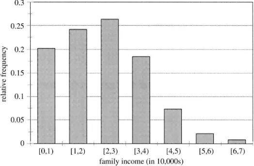
The histogram of family income in Figure 1 reveals that many students come from very poor families. One-third of students have a family income in the first year of less than $15,800. Another one-third of students have a family income in the first year between $15,800 and $28,020. Most of the remaining families have a family income in the first year of less than $50,000. Family incomes are right truncated because, as will be discussed in more detail in Section III, eligibility for admission requires that a student’s family income must be below a maximum level.
The college performance outcome that we primarily concentrate on is duration of college attendance. This is worthwhile if, as research such as Kane and Rouse (1995) suggests, completing some college leads to an increase in a person’s earning poten-tial. Another reason to study duration rather than the binary college graduation
out-15. Most individuals in our sample took the ACT exam. In cases where a student took only the Scholastic Aptitude Test (SAT), the student’s SAT scores were converted to ACT ‘‘equivalents.’’ In Section IV we discuss the interpretation of our results given the use of math ACT and verbal ACT as ability measures. A student’s distance from home is potentially endogenous. However, removing this variable had very little effect on the estimated importance of the other characteristics.
16. The number of individuals who had missing values of each variable is: sex⫽17, race⫽64, family income⫽58, math ACT⫽54, verbal ACT⫽54, and family size⫽11. For each variable, a probit model was estimated with an indicator of ‘‘whether or not the variable was missing’’ for a particular person as the dependent variable and the set of other variables as the independent variables. No evidence was found that variables are missing in systematic ways.
Figure 1
Relative frequency of family income in 1997 dollars
come is that, because all students who have not finished a degree by the end of the fall semester of 1997 are right censored in our data, concentrating directly on the latter would seriously limit the amount of useable data. For example, even under the assumption that no students take more than five years to graduate, it is not possi-ble to determine graduation outcomes for individuals who matriculated after the first three years of our data. Ignoring the last five years of data is inefficient because these years contain useful information about the likelihood of college completion.
Although students can choose to leave school at any time during the school year, the data do not indicate the exact date at which a student leaves. Instead, we observe the semester in which the person leaves. Starting in the seventh semester after matric-ulation, some students begin to graduate. In order to avoid the complication of model-ling both the attendance duration and the exit reason, the focus of the empirical work in this paper is on student retention up until the start of the seventh semester.18
Stinebrickner (1998) shows that almost all individuals in this sample who return for the start of their fourth year (and are not censored) eventually graduate.19Therefore,
beginning the seventh semester is almost synonymous with graduation.
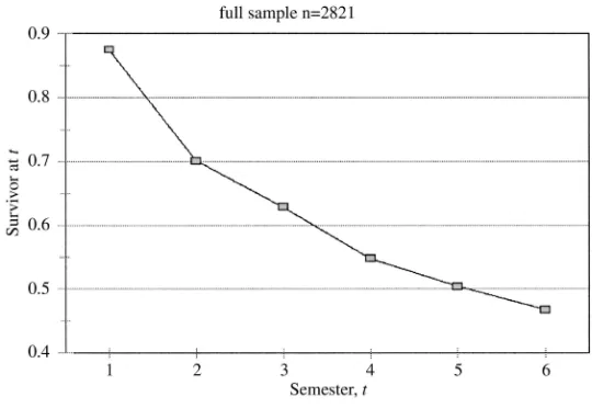
Figure 2 shows a nonparametric Kaplan-Meier survivor function for the duration of time that an individual in our sample remains in college. The survivor function evaluated at timetrepresents the probability that a student will stay more thantfull semesters before leaving school (that is, he will start at least thet⫹1stsemester).
The probability that an individual will stay more than six full semesters (start his seventh semester) is approximately 0.47. Thus, approximately half of entering
stu-18. For the empirical work, individuals who persist until the seventh semester are artificially censored at this point.
Stinebrickner and Stinebrickner 599
Figure 2
Kaplan-Meier survivor function
dents at Berea do not graduate even though the burden of paying for college has been removed as a possible cause of attrition.
The previous results show that many students do not graduate and that exits are for reasons unrelated to the direct costs of college. It is worth noting that what is likely to be of ultimate interest from a policy standpoint is whether individuals even-tually receive a degree at this school or another four-year institution. However, the difference between educational attainment at Berea and total post-secondary educa-tional attainment appears to be relatively small. In correspondence with the director of institutional research at Berea College, it was learned that exit interviews taken in recent years show that only approximately 0.17 of exiting students express some intent to transfer to another two-year or four-year post-secondary institution. Further, the majority of these students never actually request a transfer transcript which, in most cases, is a necessary condition for actually transferring.
III. The Relationship between Family Income and
College Outcomes at Berea
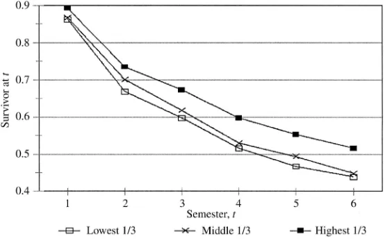
Largely because many of the students are extremely poor, a substan-tial amount of variation exists in the family incomes of the students in our sample. In this section, we take advantage of this variation to examine whether the type of positive relationship between family income and college attrition that has consis-tently been found in the literature remains in a situation where the potential burden associated with paying for college has been removed.20Kaplan-Meier survivor
Figure 3
Kaplan-Meier survivor functions for three income groups
tions of the sort used in Section II indicate that this is the case. In particular, Figure 3 shows that the Kaplan-Meier survivor functions differ for individuals in the lowest third, middle third, and highest third income groups. The probability that an individ-ual in the highest third finishes more than six full semesters is 18 percent larger than the probability that an individual in the lowest income third finishes more than six full semesters (0.516 versus 0.439).
The Kaplan-Meier survivor functions do not take into account the effect that co-variates have on retention. Consequently, retention differences among the income groups may be the result of differences in other observed characteristics that make students less likely remain in school. Table 1 shows descriptive statistics for the overall sample and each of the income thirds. In general, the variable means are quite similar across income groups. This result suggests that retention differences between income groups are likely to remain even after taking into account other observable characteristics. This can be verified using a proportional hazard model. The hazard,hi(t), represents the probability that a person will leave school at time
tconditional on not having left before timet
(1) hi(t)⫽exp(βXi⫹εi ⫹B(t))
whereβis a set of coefficients which measure the effect of the exogenous characteris-ticsXion the hazard rate,εirepresents a person specific heterogeneity term, and the
baseline hazard B(t) indicates how the hazard rate changes with the duration of attendance. Identification of the proportional hazard model requires that the baseline hazard be separable from other covariates. The primary results in the paper come from a specification that includes a nonparametric baseline and a parametric (normal)
Stinebrickner
and
Stinebrickner
601
Table 1
Data Description—Full Berea Sample and Berea Sample Divided into Income Thirds, n⫽2,821
Lowest 1/3 Middle 1/3 Highest 1/3
Full Sample Income Mean Income Mean Income Mean
Mean Standard Standard Standard Standard
Deviation Deviation Deviation Deviation
Income/1,000 2.245 1.359 0.767 0.527 2.201 0.345 3.770 0.729
Male 0.454 0.446 0.439 0.476
Black 0.1 0.131 0.087 0.082
Verbal ACT 22.172 4.361 21.887 4.335 22.143 4.180 22.487 4.544
Math ACT 20.410 3.859 20.123 3.828 20.385 3.854 20.723 3.877
Distance from home—close 0.39 0.388 0.38 0.415
distribution for the unobserved heterogeneity.21However, as discussed in footnote
23, the results were found to be very similar when the model was specified with a flexible form for the unobserved heterogeneity of the type proposed by Heckman and Singer (1984).
Table 2 shows the maximum likelihood estimates of the proportional hazard model. Column 1 shows estimates when family income enters as a continuous vari-able. Column 2 shows estimates when the effect of income is estimated semiparamet-rically by including an indicator variable for whether a person’s family income places him in the lowest third income group and an indicator variable for whether the per-son’s family income places him in the middle third income group. Column 3 shows estimates when the effect of income is estimated semiparametrically and income is divided into six different groups. Column 4 shows estimates when income enters as a continuous variable and high school grades are also included.
The coefficient associated with a particular variable can be used to compute the factor by which the hazard rate would change if the variable increased by one unit, with a negative coefficient indicating that an increase in the variable would be associ-ated with a lower probability of leaving. For example, the coefficient on Math ACT,
⫺0.051, indicates that the hazard rate decreases to exp(⫺0.051)⫽0.950 of its previ-ous value when the Math ACT score increases by one point.
Table 2 indicates that family income has a highly significant effect, even after controlling for the effect of educational background variables and other observable characteristics. Column 1 shows that a $10,000 increase in family income leads to a hazard rate that is lower by a factor of exp(⫺0.083)⫽0.920.22For a ‘‘baseline’’
student, Figure 4 compares the predicted survivor function for a family income of $5,000 to the predicted survivor function for a family income of $40,000.23 The
probability that the person with a $40,000 family income remains in school for more than six full terms is 25 percent higher than the probability that the person with $5,000 in family income remains in school more than six full terms (0.520 versus 0.416).24Column 2 shows that the income coefficients are also statistically significant
and quantitatively large when income enters as two indicator variables. A person in the lowest income group and middle income group have hazard rates which are exp(0.243)⫽1.275 and exp(0.201)⫽1.222 as large as the hazard rate of an individ-ual in the highest income group holding all other observable characteristics constant.
21. The baseline hazard is assumed to be constant within each of the semesters. The value of each of these constants is estimated.
22. As mentioned earlier, very little change was found when the model was specified with a flexible form for the unobserved heterogeneity of the type proposed by Heckman and Singer (1984). For example, for the specification in Column 1 of Table 2, whenεiis assumed to be a discrete random variable with two possible values it was found that the estimated effect (standard error) of family income is⫺0.084 (0.024) and the value of the log likelihood function is⫺3,484.05. The full results for this specification in the Appendix Table A1 show that estimated effects are also very similar for other observable variables. Similar results were found when the number of possible values allowed forεiwas increased, and, as a result, these specifications are not shown. Although the results are not shown, the results in Columns 2-4 of Table 2 were also found to be robust to the specification of the unobserved heterogeneity term.
23. The baseline person was given the mean values of the continuous covariates and was given median values for the indicator variables.
Stinebrickner
Variable Estimate SE Estimate SE Estimate SE Estimate SE
Male 0.242a (0.67) 0.240a (0.067) 0.243 (0.067) 0.068 (0.073)
Black ⫺0.157 (0.104) ⫺0.149 (0.104) ⫺0.152 (0.105) ⫺0.306a (0.123)
High school GPA ⫺0.616a (0.094)
Verbal ACT ⫺0.017 (0.008) ⫺0.017a (0.008)
Family size 0.004 (0.020) 0.001 (0.020) 0.016 (0.023) 0.014 (0.023)
Distance from home—close ⫺0.024a (0.065)
⫺0.202a (0.065)
⫺0.202a (0.065)
⫺0.118 (0.072)
Income/10000 ⫺0.083a (0.024)
⫺0.095a (0.027)
Indicator for income in bottom 1/3 0.243a (0.079)
Indicator for income in middle 1/3 0.201a (0.78)
Indicator for income in bottom 1/6 0.323a (0.112)
Income in 2nd1/6 0.329a (0.112)
Income in 3rd1/6 0.291a (0.112)
Income in 4th1/6 0.222a (0.112)
Income in 5th1/6 0.127a (0.112)
Variance of heterogeneity 0.297 (0.605) 0.284 (0.078) 0.310 (0.469) 0.511 (0.298)
t⫽1 ⫺2.223a (0.184)
Log likehood ⫺3,484.936 ⫺3,485.801 ⫺3,484.61 ⫺3,009.676
a
t-statistic greater than 2.0.
The first three columns are models estimated without high school grade point averages.
Figure 4
Predicted Survivor Functions for baseline person by income
Figure 5 shows how the predicted survivor function for the baseline person varies depending on whether the person is in the lowest, middle, or highest income group. Column 3 shows that, when income is divided into six groups, retention rates are quite similar for the bottom three income groups but increase significantly over the upper half of the income distribution at Berea.
It is important to note that the unmeasured determinants of family income and schooling attainment may be different in our sample than it would be in various
Figure 5
Stinebrickner and Stinebrickner 605
populations of interest. The types of biases that may be present from viewing the relationship between family income and college attrition at Berea as an estimator of the relationship in larger populations of interest is discussed in detail in Stinebrick-ner and StinebrickStinebrick-ner (2000).25
It is worthwhile to keep in mind that the income variable used in the preceding analysis, family income at the time of matriculation, is a noisy measure of the desired variable, permanent family income. In particular, one might be concerned with the possibility that nonclassical measurement error could be generated through the in-come threshold that is used to determine which students are eligible for admission. At low levels of permanent income, it seems likely that few households will experi-ence shocks such that their first-year family incomes make them ineligible for admis-sion. As a result, average first-year family income for the lower income groups might be expected to be very similar to average permanent family income. However, for individuals with levels of permanent income that are slightly below the income threshold, positive shocks will make them ineligible for admission, and, for individuals with levels of permanent income that are above the income threshold, negative shocks will be needed for them to enter the sample. As a result, average first-year family income for the high-income group might be expected to be lower than average permanent family income. If this scenario is true, it is possible that the associated bias could lead to an undesirable overstatement of the effect of income on duration in the model where income enters as a continuous variable. However, our investigations into this matter did not produce evidence that the income threshold causes this type of problem.26
IV. Interpretation of Berea Results—Reasons for
Attrition Differences Between Income Groups
Section III indicates that statistically significant and quantitatively large differences exist in retention rates between income groups at Berea even in the presence of the full subsidy. From the standpoint of designing effective policy
programs, it would be desirable to determine which of the possible reasons related to family environment that were discussed in the introduction are most plausible. In this section, we attempt to examine this issue using our data from Berea.
Without additional information, conclusions about the reasons behind the differ-ences by family income depend to a large extent on the interpretation of our measures of ability, the ACT math and verbal exams. For example, consider one extreme in which the ACT exams are essentially types of IQ tests that predominantly measure a person’s inherent ability at birth and are largely unaffected by a person’s formal and informal educational environments while growing up. In this scenario, from the standpoint of graduation probabilities for those who matriculate, the size of the difference between income groups can reasonably be thought of as the full disadvan-tage of being born into a low-income family. That is, the disadvandisadvan-tage which is attributable to any of the reasons discussed in the introduction: differences in educa-tional opportunities and preparation, differences in parental support and encourage-ment during a person’s college career, or differences in family responses to income shocks that are unrelated to the costs of college.
In reality it is certainly true that ACT scores to some extent also capture the amount of learning that takes place during a student’s youth. However, to the extent that this endogeneity exists, from the standpoint of graduation probabilities for those who matriculate, it seems reasonable to believe that the size of the retention differences between income groups is a conservative estimator of (understates) the true lifetime disadvantage of being born into a low-income family. The reason for this is simply that the test scores of students from low-income families will tend to understate these students’ inherent ability if students from low-income families suffer on aver-age from inferior learning environments when young. Thus, the retention differences between students from high-income families and low-income families would be found to be even larger if it was possible to control for ‘‘true’’ ability levels at birth rather than the potentially endogenous ACT scores. However, even if the scores are potentially endogenous, we would be able to rule out the possibility that differences in educational opportunities for youth in different income groups cause the income differences in retention if we believed that these test scores are able to fully capture the aspects of learning/ability that are relevant for college. However, this is not necessarily the case. For example, the math portion of the ACT exam certainly mea-sures something about a person’s quantitative background and ability, but is likely to only indirectly indicate whether an individual had the opportunity to take a calcu-lus class while in high school.
Thus, while the previous paragraphs seem to suggest that our estimates of the influence of family income on college completion will be somewhat conservative if test scores depend endogenously on family income, they do not shed much light on the reasons for the income differences in retention rates that remain even in the presence of the full tuition subsidy. In the remainder of this section we attempt to more directly explore the plausibility of possible explanations.
A. Grades and Academic Preparation
Stinebrickner and Stinebrickner 607
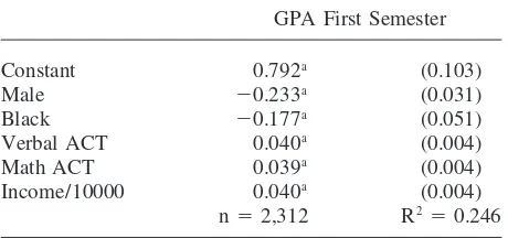
Table 3
Regression of College Grades in First Semester—Berea Sample For All Students Who Completed First Semester, n⫽2,661
GPA First Semester
Constant 0.792a (0.103)
Male ⫺0.233a (0.031)
Black ⫺0.177a (0.051)
VerbalACT 0.040a (0.004)
MathACT 0.039a (0.004)
Income/10000 0.040a (0.004)
n⫽2,312 R2
⫽0.246
entrance exam scores. Semester by semester college grade regressions suggest that this is true. For example, Table 3 shows the results of a regression of the first semester college grade point average (GPA) on observable personal characteristics for all individuals who finished their first term. The coefficient on family income, 0.040, implies that the GPA of an individual with a family income of $40,000 is on average 0.16 higher than an individual with $0 of family income holding other observable characteristics constant.27Further, the coefficient is statistically significant with at
-statistic of 10.0. Although the regression results are not shown, the effect of family income on term grade point average is also significant (at a 0.10 level of significance or lower) for four of the subsequent five semesters with point estimates of 0.023, 0.036, 0.041, 0.014, and 0.028.28The pooled regression involving all grades in all
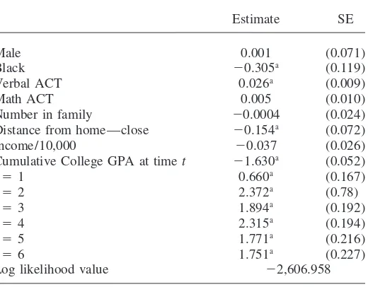
semesters produces a point estimate of 0.033 and an associatedt-statistic of 4.013. From the standpoint of retention, whether these effects are quantitatively large depends on the nature of the relationship between grades and retention. Thus, to get a sense of the extent to which these grade differences between income groups ‘‘ex-plain’’ the family income differences in retention that were found earlier, the duration model was estimated including cumulative grade point average as a time-varying covariate.29The coefficient on cumulative grade point average in Table 4 indicates
27. The mean and standard deviation of students’ grade point averages in the first period are 2.464 and 0.856 respectively.
28.p-values are 0.048, 0.002, 0.001, 0.277, and 0.048 respectively. The grade differences are consistent with (but somewhat larger) than the findings of Betts and Merrall (1999) who analyze the relationship between first-semester grades and family background for students at the University of California at San Diego. Bowen and Bok (1998) also find a positive relationship between socioeconomic status and college grades.
Table 4
Proportional Hazard Model of Attrition Including Cumulative College Grade Point Average—Berea sample, n⫽2,649
Estimate SE
Male 0.001 (0.071)
Black ⫺0.305a (0.119)
Verbal ACT 0.026a (0.009)
Math ACT 0.005 (0.010)
Number in family ⫺0.0004 (0.024)
Distance from home—close ⫺0.154a (0.072)
Income/10,000 ⫺0.037 (0.026)
Cumulative College GPA at timet ⫺1.630a (0.052)
t⫽1 0.660a (0.167)
t⫽2 2.372a (0.78)
t⫽3 1.894a (0.192)
t⫽4 2.315a (0.194)
t⫽5 1.771a (0.216)
t⫽6 1.751a (0.227)
Log likelihood value ⫺2,606.958
aRepresents
t-statistic greater than two.
Sample size is smaller than sample size in Table 2 because the 172 students who did not stay in school long enough to receive first semester grades are not used in the analysis.
that poor grades are a very significant predictor of exits from school. If college GPA increases by a full point, the hazard rate decreases to exp(⫺1.630)⫽0.195 of the previous value. A comparison of Table 4 with the fist column of Table 2 shows that the effect of income decreases substantially (from⫺0.083 to⫺0.037) and becomes statistically insignificant when grades are taken into account.30
Although it is clear that college grades are strongly related to exits from school and that lower-income students receive lower average college grades, one must be very cautious about what conclusions are drawn from this information. Certainly, one plausible story is that grades are essentially exogenous to the dropout decision, in which case it would be reasonable to conclude that differences in college grade performance between income groups are caused by unmeasured differences in aca-demic preparation or study skills between income groups. However, another
Stinebrickner and Stinebrickner 609
ity is that students who are unhappy at college and/or are planning to drop out may receive lower grades simply because they are less focussed on their studies than they otherwise would be.31
While it is typically difficult to credibly separate the relative importance of the two effects, there does seem to be evidence that the latter endogeneity explanation is not the driving force. Although the full results are not shown, the estimated effect andt-statistic of family income on the cumulative grade point average at the begin-ning of the seventh semester for the 963 sample members who remained in school until their seventh semester are 0.028 and 2.9 respectively.32Thus, income is a
sig-nificant predictor of cumulative grade point average even though members of this group are very likely to graduate, and, as a result, should be relatively unaffected by the type of grade endogeneity described above. Further, because the effect of income on grades for this group is found to be roughly constant across semesters, it does not appear that the difference in cumulative grades in the seventh semester is simply due to the low-income individuals in this group adjusting more slowly to college.33Thus, the grade data does seem to provide at least some evidence that
low-income individuals are at a disadvantage because of their educational backgrounds, even after taking into account college entrance exam scores.
As discussed earlier, students from low-income families could be less prepared for college because they receive inferior formal educational instruction or because they receive inferior educational instruction at home. In an effort to provide some information about the relative importance of the two possibilities, we concentrate on the 1,188 students in the sample from the state of Kentucky. The benefit of study-ing this group is that, for each school year between 1991–92 and 1996–97, a measure of school quality was constructed under the Kentucky Instructional Results Informa-tion System (KIRIS) in order to ‘‘provide financial incentives for districts, schools, and teachers to make progress toward specific goals.’’34We obtain a single school
quality measure for each district by averaging the six yearly ratings. This single measure has a mean of 41.107 and a standard deviation of 2.807. The district ratings used here combine ratings for elementary, secondary, and high schools and involve weighted averages of things such as student test scores, attendance rates, retention rates, dropout rates, and the rate at which students ‘‘successfully’’ transition after
31. Another possible explanation is that students from low-income families may be forced to spend more time working in nonacademic jobs. This can be examined directly using the administrative data because Berea College operates a mandatory work-study program, does not allow students to work off-campus, and maintains students’ work records as part of its administrative database. By taking advantage of the existence of random assignment to freshmen jobs, Stinebrickner and Stinebrickner (2003), find a quantitatively large (and statistically significant) negative effect between working and grade performance. However, because no relationship between family income and hours-worked is found, the results indicate that differences in employment do not explain differences in grades that exist between different income groups.
32. The regressors are the same as in Table 3.
33. The point estimates on the income coefficient in a semester by semester regression of semester grades on observable characteristics for those individuals who persist until seventh semester are 0.025, 0.021, 0.022, 0.027, 0.021, and 0.028 respectively. The associatedpvalues are 0.054, 0.083, 0.080, 0.025, 0.112, and 0.048.
graduation from high school. Thus, the rating for a particular district will capture both school quality and the ability/home learning environment of students in the district.
A $10,000 increase in family income is estimated to increase a person’s school rating by 0.342 with an associatedt-statistic of 5.941. Thus, students from the lower income families do attend schools with somewhat lower ratings. Although the full results are not shown, the estimated coefficient andt-statistic associated with the school quality variable from a pooled regression involving all semester grades in all years for the KY subsample are 0.017 and 3.034 respectively.35Thus, higher school
ratings are related to significantly higher college grades. Nonetheless, the estimated effect of family income on college grades remains large for the KY subsample when the school quality measure is included; the point estimatet-statistic are 0.038 and 3.160 respectively.36
Although this would seem to suggest that the effect of family income on attrition will remain strong even after taking into account the school ratings, there are plausi-ble nongrade avenues through which the school ratings could affect student attrition. For example, student from schools with higher ratings will tend to have more friends or classmates who are also attending college, and, as a result, may view leaving college before completion to return home as less desirable than other students. In an attempt to capture both the effect that good schools have on college grades and these other types of effects, we estimated the duration model for the KY sub-sample including both the observable characteristics in Column 1 of Table 2 and the school quality measure. Because the estimated effects of the majority of the variables are very similar to those in Column 1 of Table 2, the entire set of results is not included. However, the coefficient andt-statistic associated with the school quality variable was found to be ⫺0.034 and 1.98. Thus, students from inferior schools do leave more quickly even after taking into account the other observable characteristics. However, the estimated effect of family income remains very im-portant and school quality is not found to account for much of the difference in attrition between students from different income situations. When the school quality measure is not included, the point estimate and t-statistic associated with the family income for the KY subsample are ⫺0.115 and ⫺3.40 respectively. When the school quality measure is included, the point estimate andt-statistic de-cline to⫺0.106 and 3.11 respectively. Adding additional controls to the specification did not change the results in any important way.37 Certainly it is possible that a
35. The set of observable characteristics includes the school quality variable and the set of variables in Table 3. There are 1,117 individuals and 4,569 total observations. Standard errors are adjusted to reflect the pooled nature of the data.
36. When the school quality measure is not included, the point estimate andt-statistics for the KY subsam-ple are 0.043 and 0.3666 respectively.
Stinebrickner and Stinebrickner 611
nontrivial amount of measurement error exists in the school ratings.38Nonetheless,
the results seem to suggest that families have a very strong direct effect on their children.
B. Negative Income Shocks to Family Income
In the introduction, an argument was made that negative income shocks may have differential retention effects on low-income students, even if direct costs are zero. Until this point, the analysis has utilized the student’s family income in the year that a student matriculated to college. However, the data also contain additional information about family income in the subsequent years of attendance. Thus, by adding a time varying ‘‘change in family income’’ variable,∆income, and an inter-action of this variable with the family income variable to the proportional hazard specification in the first column of Table 2 it is possible to some extent to examine whether negative income shocks influence the attendance decision when a full sub-sidy is in place and to examine to what extent the effect of income shocks differ by income. This exercise did not produce any evidence that negative income shocks have a significant effect on the timing of exits.39
Although this suggests that differences between income groups are not being caused by differential responses to income shocks, it is important to note that the measurement error, created by the timing of when family income is measured, will lead to parameter bias in the analysis. The income data come directly from the yearly FAFSA form, which must be submitted by the student sometime between January 1 and April 15 and corresponds to a family’s W2 income form from the previous year. We make the assumption that the first reported yearly income is the relevant income for the fall semester of the person’s first year. We make the assumption that the second reported income is the relevant income for the spring semester of the first year and the fall semester of the second year. Similarly, the third reported income corresponds to the fourth and fifth semesters and the fourth reported income corre-sponds to the sixth semester.
Essentially, the income values that we associate with the two semesters in a given calendar year come from the family’s W2 form from the previous calendar year. To the extent that we are interested in the effect of income shocks, it seems likely that this timing assumption will lead to a downward bias for the estimator of the effect of income shocks with the extent of the bias depending on the extent to which income shocks tend to cause students to exit very quickly.40
38. For example, it is likely that the ratings were not designed to exclusively measure college prepara-tion.
39. The estimated effect (standard error) of the∆income variable in this specification was⫺0.010 (0.023) and the estimated effect (standard error) of family income was⫺0.098 (0.028). Adding an interaction term between family income and∆income did not change the nature of the results. The sample size was 2,446.
V. A Comparison to Students who Pay Tuition
The total relationship between family income and college attrition that has been found in the literature is the sum of the portion due to the family environment explanation and the portion due to the direct costs explanation (assum-ing that selection bias has been accounted for or is not important). Section III sug-gests that the family environment effect is important. However, because tuition is zero for everyone at Berea, the Berea data cannot provide direct evidence about the importance of the direct costs explanation. In an effort to provide an idea of the size of the total relationship between family income and college outcomes (and, thus, a rough idea of the importance of the family environment explanation relative to the direct costs explanation), we estimate the duration model of attrition using data from the NELS-88. These data sustain continuing trend comparisons with the National Longitudinal Study of the High School Class of 1972 and the High School Beyond (1980), which were used by Manski and Wise (1983) and Manski (1992), and are a logical choice because students who made normal progress through high school and entered college soon after graduation would have matriculated during the middle of the sample period covered by our Berea data.
There are 2,823 students in the NELS-88 who entered a bachelor degree program at a four-year (private or public) college in the fall of 1992 or the fall of 1993. In order to make the NELS-88 sample more similar in nature to the Berea sample, we remove 684 individuals in the data who have a family income above $85,800 in 1997 dollars. After also removing individuals with missing values of family income or of other characteristics that are used in the analysis, we are left with 1,468 individ-uals.41
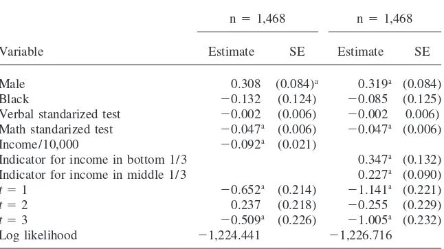
The analogs to Column 1 and Column 2 of Table 2 are shown in Table 5.42In
both cases, the estimated effects of family income are very similar to those in Table 2,
January-April period before the school year started. However, this change increases the income measure-ment error due to the timing of income measuremeasure-ments. In practice, this change made very little difference in the model estimates.
41. The variables used in this analysis are indicators for male and black, a math standardized test score, a reading standardized test score, and family income. Of the ‘‘income-eligible’’ students, 383 have a missing family income, 399 have a missing standardized reading score, and 397 have a missing standard-ized math score.
42. The family income variable in the NELS-88 is categorical. To estimate the analog of Column 2 of Table 2 (in which family income is categorical), we define the low-income variable to include all incomes less than 17,160 and we define the high-income variable to include all incomes greater than 40,040.
To estimate the analog of Column 1 of Table 2 (in which family income enters as a continuous variable), because the exact income value is not observed, we first fit a lognormal distribution to the categorical data (using both the individuals in the sample used to estimate Table 5 and the individuals that were removed from the final sample due to higher family incomes). We then compute the likelihood contribution for person i by integrating the likelihood contribution conditional on the person’s family income (from Appen-dix Table A1) over the appropriate distribution of the person’s family income given the estimated lognormal distributions and the person’s family income category. We found very similar results (that is, point estimate andt-statistic of⫺0.071 and⫺2.95 respectively) when we estimated the continuous case by simply making the assumption that the family income of each person in a particular income class is equal to the midpoint of that class.
Stinebrickner and Stinebrickner 613
Table 5
Proportional Hazard Model of Attrition—NELS–88
n⫽1,468 n⫽1,468
Variable Estimate SE Estimate SE
Male 0.308 (0.084)a 0.319a (0.084)
Black ⫺0.132 (0.124) ⫺0.085 (0.125)
Verbal standarized test ⫺0.002 (0.006) ⫺0.002 0.006)
Math standarized test ⫺0.047a (0.006)
⫺0.047a (0.006)
Income/10,000 ⫺0.092a (0.021)
Indicator for income in bottom 1/3 0.347a (0.132)
Indicator for income in middle 1/3 0.227a (0.090)
t⫽1 ⫺0.652a (0.214)
⫺1.141a (0.221)
t⫽2 0.237 (0.218) ⫺0.255 (0.229)
t⫽3 ⫺0.509a (0.226)
⫺1.005a (0.232)
Log likelihood ⫺1,224.441 ⫺1,226.716
at-statistic greater than 2.0.
despite the fact that the students in the NELS-88 are attending tuition-charging insti-tutions.43Thus, although one should be very careful about drawing conclusions from
this comparison, the exercise suggests that family environment factors may be the driving force in determining the strong relationship between family income and edu-cational outcomes. However, it is important to note that the effect of direct costs under current tuition/financial aid programs is influenced by both the possibility that low-income students find paying direct costs burdensome for reasons such as liquid-ity constraints and the realliquid-ity that students from low-income families are likely to face lower direct cost due to the existence of need-based financial aid. The former suggests that low-income students will tend to leave schools more quickly. The latter suggests that low-income students will leave school less quickly. Thus, even if the total effect of direct costs on college outcomes is close to zero, this does not imply that liquidity constraints are unimportant for low-income students.
43. Figure 4 shows that the predicted survivor function att⫽3 (probability of finishing more than three full semesters) at Berea is 0.67 if the person has family income of $40,000 and is 0.58 if the person has family income of $5,000. For the NELS-88 sample, these number are 0.72 and 0.63 respectively.
It seems possible that many of the possible reasons related to the family environ-ment effect would be as closely related to parental education backgrounds as they would be to family income per se. Unfortunately, information regarding parental education is not available in our Berea data. However, this information is available in the NELS-88. When we estimated the specification in Column 1 of Table 5 with an additional indicator of whether the student had at least one parent who had obtained a college degree, we found that this variable was statistically significant with a point estimate of⫺0.36 and at-statistic of⫺3.02. The estimated effect of family income declined to⫺0.062 but remained statistically significant with at-statistic of⫺2.859.
VI. Conclusion
Bowen and Bok (1998) raise the possibility that low national gradua-tion rates may be due to the inability of students and their families to meet college costs. The high overall attrition rates at Berea College, where all students receive a full tuition subsidy (and pay an average of approximately $1,000 for room, board, and college fees), suggest that college exits often occur for reasons that are unrelated to the direct costs of college. It is important to note that it is necessary to be cautions about drawing inference about more general populations of interest on the basis of a single school. Nonetheless, given the statistically significant and quantitatively large relationship that is found between family income and performance at Berea, the discussion of the possible sources of bias that might be present in our Berea estimator that appears in Stinebrickner and Stinebrickner (2000), and the comparison to outcomes in the NELS-88, this work suggests that reasons related to family envi-ronment are the most important determinants of the differences in college outcomes by family income that have consistently been found in the literature.
Stinebrickner and Stinebrickner 615
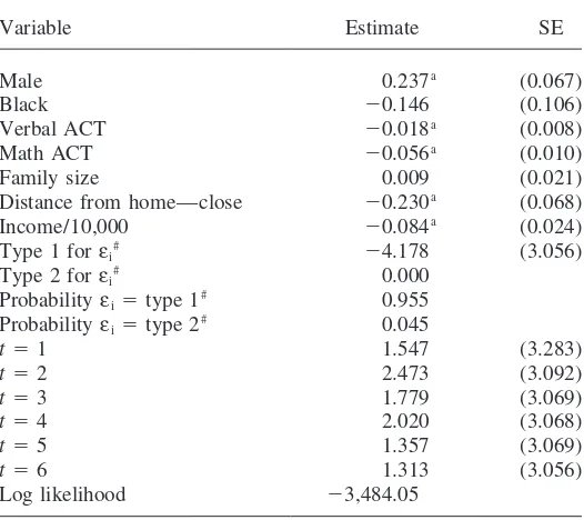
Table A1
Proportional Hazard Model of Attrition with Heckman-Singer Heterogeneity—Berea Sample, n⫽2,821
Variable Estimate SE
Male 0.237a (0.067)
Black ⫺0.146 (0.106)
Verbal ACT ⫺0.018a (0.008)
Math ACT ⫺0.056a (0.010)
Family size 0.009 (0.021)
Distance from home—close ⫺0.230a (0.068)
Income/10,000 ⫺0.084a (0.024)
Type 1 forεi# ⫺4.178 (3.056)
Type 2 forεi# 0.000
Probabilityεi⫽type 1# 0.955
Probabilityεi⫽type 2# 0.045
t⫽1 1.547 (3.283)
t⫽2 2.473 (3.092)
t⫽3 1.779 (3.069)
t⫽4 2.020 (3.068)
t⫽5 1.357 (3.069)
t⫽6 1.313 (3.056)
Log likelihood ⫺3,484.05
at-statistics greater than 2.0.
Results are analogous to those in Column 1 of Table 2, but specification involves Heck-man-Singer flexible form for unobserved heterogeneity.
#type 2 forεiis normalized to zero. To ensure that Pr(εi⫽type 1) and Pr(εi⫽type 2) are nonnegative and sum to one we define Pr(εi⫽type 1)⫽eγ/(eγ⫹e0), Prεi⫽ type 2)⫽e0/(eγ⫹e0) and estimateγ. Point estimate (standard error) ofγare 3.048* (0.854).
References
Belman, Dale, and John S. Heywood. 1991. ‘‘Sheepskin Effects in the Returns to
Educa-tion: An Examination on Women and Minorities.’’Review of Economics and Statistics
73(4):720–24.
———. 1997. ‘‘Sheepskin Effects by Cohort: Implications of Job Matching in a Signalling
Model.’’Oxford Economic Papers49(4):623–37.
Betts, Julian, and Darlene Merrall. 1999. ‘‘The Determinants of Undergraduate Grade Point Average: The Relative Importance of Family Background, High School Resources,
and Peer Group Effects.’’The Journal of Human Resources34(2):268–93.
Bound, John, and George Johnson. 1992. ‘‘Changes in the Structure of Wages in the
1980’s: An Evaluation of Alternative Explanations.’’The American Economic Review
Bowen, William, and Derek Bok. 1998.The Shape of the River. Princeton, N.J.: Princeton University Press.
Cameron, Stephen V., and James Heckman. 1998. ‘‘Life Cycle Schooling and Dynamic
Se-lection Bias: Models and Evidence for Five Cohorts of American Males.’’Journal of
Po-litical EconomyApril: 262–333.
Cameron, Stephen V., and Christopher Taber. 1999. ‘‘Borrowing Constraints and the Re-turns to Schooling.’’ Unpublished.
Card, David, and Alan Krueger. 1992. ‘‘Does School Quality Matter? Returns to Education
and the Characteristics of Public Schools in the United States.’’Journal of Political
EconomyFebruary: 1–42.
Cohn, E., and B.F. Kiker. 1986. ‘‘Socioeconomic Background, Schooling, Experience and
Monetary Rewards in the United States.’’Economica53:497–503.
Daniel, Kermit, Dan Black, and Jeffrey Smith. 1997. ‘‘College Quality and the Wages of Young Men.’’ Unpublished.
———. 1995. ‘‘College Characteristics and the Wages of Young Women.’’ Unpublished. Grogger, Jeff, and Derek Neal. 2000. ‘‘Further Evidence on the Benefits of Catholic
Sec-ondary Schooling.’’Brookings-Wharton Papers on Urban Affairs1:151–93.
Hauser, R. M. 1973. ‘‘Socioeconomic Background and Differential Returns to Education.’’ InDoes College Matter, ed. L. Solomon. New York: Academic Press.
Havemen, Robert H., and Barbara Wolfe. 1984. ‘‘Schooling and Economic Well-Being:
The Role of Nonmarket Effects.’’The Journal of Human Resources19(3):377–
407.
Heckman, J., and B. Singer. 1984. ‘‘A Method for Minimizing the Impact of Distributional
Assumptions in Econometrics Models for Duration Data.’’Econometrica52:271–320.
Heckman, James, Lance Lochner, and Christopher Taber. 1998. ‘‘Tax Policy and Human-Capital Formation.’’ American Economic Review 88(2):293–97.
———. 1998. ‘‘General-Equilibrium Treatment Effects: A study of Tuition Policy.’’
Ameri-can Economic Review88(2):381–86.
Heywood, John S. 1994. ‘‘How Widespread are Sheepskin Returns to Education in the
U.S.?’’Economics of Education Review13(3):227–34.
Hungerford, Thomas, and Gary Solon. 1996 ‘‘Sheepskin Effects in the Returns to
Educa-tion.’’Review of Economics and Statistics69(1):175–77.
Jaeger, David A. and Marianne E. Page. 1996. ‘‘New Evidence on Sheepskin Effects in
the Return to Education.’’Review of Economics and Statistics78(4):733–40.
Johnson, William R. 1998 ‘‘Distributional Issues in the Public Support of Higher Educa-tion.’’ Unpublished.
Kane, Thomas J. 1994. ‘‘College Entry by Blacks since 1970. The role of College Costs,
Family Background, and the Returns to Education.’’Journal of Political Economy
102(5):878–911.
Kane, Thomas J., and Cecilia Rouse. 1995. ‘‘Labor Market Returns to Two and Four Year
College.’’American Economic Review85(3):600–14.
Katz, Lawrence, and Kevin Murphy. 1992 ‘‘Changes in Relative Wages, 1963-1987:
Sup-ply and Demand Factors.’’The Quarterly Journal of Economics107(1):35–78.
Keane, Michael, and Kenneth Wolpin. 1998. ‘‘The Effect of Parental Transfers and Bor-rowing Constraints on Educational Attainment.’’ Unpublished.
Kiker, B.F., and C.M. Condon. 1981. ‘‘The Influence of Socioeconomic Background on
the Earnings of Young Men.’’Journal of Human Resources16(4):442–48.
Lavy, V., Michael Palumbo, and Steven Stern. 1998. ‘‘Simulation of Multinomial Probit
Probabilities and Imputation of Missing Data.’’ InAdvances in Econometrics, ed.
Thomas Fomby and R. Carter Hill. JAI Press.