How Much is Opportunities?
Helena Skyt Nielsen
Michael Svarer
a b s t r a c t
Individuals match on length and type of education. We find that around half of the systematic sorting on education is explained by the tendency of individuals to marry someone who went to the same educational institution or to an institution near them. This may be due to low search frictions or selection of people with the same preferences into the same institutions. The residual half of the systematic sorting on education is a direct effect of partners’ education, which is potentially explained by complementarities in household production in couples with same education.
I. Introduction
The decision of who to marry is for many people one of the most im-portant choices they make during their entire life. In addition, the sorting of marriage partners greatly influences a number of important economic outcomes such as in-come inequality (Aiyagari et al. 2000; Fernandez and Rogerson 2001; Fernandez et al. 2005); values, preferences, and skills of couples’ children (Becker and Murphy 2000); marital stability and female labor supply (Dalmia and Lawrence 2001); and fertility (Boulier and Rosenzweig 1984). Taking a closer look at marital sorting pat-terns reveals that couples typically match positively on individualsÕtraits. This is, in
Helena Skyt Nielsen is a professor of economics and management at Aarhus University. Michael Svarer is a professor of economics and management at Aarhus University. Helena Skyt Nielsen thanks the Danish Research Agency for support. Michael Svarer thanks the Danish National Research Foundation for support through its grant to CAM. The authors are grateful to Julie Kracht, Maria Knoth Humlum and Ulla Nørskov Nielsen for invaluable research assistance, to Juanna Schrøter Joensen and two anonymous referees for useful comments and to Birgitte Højklint for reading the manuscript. Any remaining errors are the responsibility of the authors. The data used in this article can be obtained beginning May 2010 through April 2013 from Helena Skyt Nielsen, Professor, School of Economics and Management, Aarhus University, Universitetsparken, Building 1322, DK – 8000 Aarhus C, Denmark, Tel.:+45 8942 1594, E-mail: hnielsen@econ.au.dk and Michael Svarer, Professor, School of Economics and Management, Aarhus University, Universitetsparken, Building 1322, DK – 8000 Aarhus C, Denmark, Tel.:+45 8942 1598, E-mail: msvarer@econ.au.dk. Data security policy means that access can be obtained from Aarhus only.
½Submitted June 2007; accepted August 2008
ISSN 022-166X E-ISSN 1548-8004Ó2009 by the Board of Regents of the University of Wisconsin System
particular, the case for age and level of education, but also for income, height, weight, I. Q., and parents’ characteristics (see, for example, Epstein and Guttman 1984 and Schafer and Keith 1990). Next to age, education is the trait that has the highest bivariate correlation. In a recent study by Fernandez et al. (2005), the mean correlation is 0.6 based on information from household surveys from 34 countries. As education is an important determinant of most of the economic outcomes men-tioned above, it is of great interest to investigate the origins behind educational ho-mogamy. This is the purpose of this study.
A sizeable part of this literature uses cross-country and time-series variation in the correlation to describe the trends and patterns in the correlation while only hinting at some reasons for the strong relationship. It is recognized that educational homogamy may result from a preference for partners with similar education as well as from op-portunities to meet partners with a similar education. These opop-portunities are driven by educational structures and institutions (see, for example, Mare 1991; Halpin and Chan 2003). The purpose of this study is to investigate how much of the systematic relationship between the educations of the partners is explained by opportunities and how much by preferences, while exploiting the fact that we know the geographical proximity of all partners and their educational institutions at the time when they en-rolled at education. We document that around half of the systematic sorting goes through the tendency to marry people from the same educational institution or a nearby institution, and this means that up to half of the systematic sorting is a result of lower search frictions.
In relation to the opportunities explanation, educational institutions are presum-ably very efficient marriage markets. The density of potential partners is rather high (see, for example, Goldin 1992; Lewis and Oppenheimer 2000), and search frictions are therefore smaller than in other local marriage markets (see, for example, Gautier et al. 2005 for a model that analyzes the effect of search frictions on marriage market outcomes). That educational institutions function as marriage markets is also rooted in sociology. Scott (1965) and Blau and Duncan (1967) argue that parents place their children in good colleges in order to secure the social position of the family. There is also ample evidence that partnerships form in schools. Laumann et al. (1994) report—based on a U. S. survey conducted in 1992—that 23 percent of married cou-ples met their current partner in school. In a Dutch survey from 1995, 15 percent reported having met their current partner in school (Kalmijn and Flap 2001). In fact, among the different sets of shared settings (neighborhood, family overlap, work-place, etc.) the most common place for couples to meet before a partnership is in school. In the present analysis, which is based on Danish register-based data, we find that in 20 percent of the couples the two partners attended the same educational in-stitution.
It could also be the case that educational homogamy is the outcome of a decision problem solved by rational agents. That is, an individual with a similar level, and perhaps same type, of education might be preferred to an individual with a different level of education. In the following, we focus on two mechanisms for preference-based partnership choice.
First, it might be the case that the mating of different educational groupings occurs as a result of rational behavior of risk-averse agents who seek to optimize discounted utility in an environment where future income is uncertain. A number of papers
highlight the interdependence between risk sharing and marriage. In their seminal paper, Kotlikof and Spivak (1981) showed that the expected gain a risk-averse agent can expect from the risk sharing elements of marriage formation amounts to 10-20 percent of his wealth. Since then, Rosenzweig and Stark (1989), Micevska (2002), Chen, Chiang and Leung (2003), and Hess (2004), among others, have investigated related aspects of partnership formation and dissolution in association with the pres-ence of idiosyncratic income risk. The idea is that risk-averse agents can benefit from forming marriage with others to insure against unforeseen changes in income. Along the lines of Hess (2004), a good economic match has a high mean income, a low-income volatility, and an low-income process that negatively correlates with ones own income process, much like a financial asset portfolio. In the present analysis, we consider matching between individuals with different educations. The income varia-bles are generated as time-series means for different educational groupings. As a consequence, the income processes are exogenous to the specific partnership, and we implicitly assume that the agents are able to predict the future income compo-nents for different educational groups.
Second, it could also be the case that the educational attainment of spouses is a complement in the household production function. Becker (1973) argues that posi-tive assortaposi-tive mating is optimal when traits are complements. According to this ar-gument, a reason why two partners with the same education form a partnership is that they tend to appreciate the same public goods or the same kind of leisure. It is not obvious how to identify to what extent educational traits are complements in the household production function, although it is commonly assumed to be the case (see, for example, Chiappori et al. 2006). In the present analysis, we attribute the part of the realized partnership formation between individuals that cannot be explained by opportunities (that is, proximity of partners) or by portfolio choices to complemen-tarities in household production.1
In this paper, we exploit a rich register data set to disentangle the correspondence between education and marriage market behavior. We have detailed information on individuals’ educational attainment, including the exact type of education and where the education was taken. After combining with information on individual income, we investigate to which extent educational portfolios of couples are related to proximity of educational institutions, portfolio optimization, and residual explanations that en-compass complementarities in household productions. From a more general perspec-tive, the analysis allows us to evaluate whether the systematic relationship between the educations of the partners is explained by opportunities (low search frictions) or preferences (complementarities or portfolio optimization).
We find that around half of the systematic sorting on education is due to the ten-dency for people to marry someone who went to the same educational institution, or who studied near them. We cautiously interpret this as a sign of low search frictions in marriage markets of the educational institutions, although we are aware that there may also be selection of people with the same preferences into institutions. The in-come properties of the joint inin-come process show no influence on partner selection,
and therefore the other half is attributed to residual explanations of which comple-mentarities in household production are likely important.
The structure of the paper is as follows: In Section II, we describe the data set. In Section III, we take a closer look at partnership formation, and in Section IV, we con-clude.
II. Data
The data we use to test our hypotheses come from IDA (Integrated Database for Labour Market Research) created by Statistics Denmark. The informa-tion comes from various administrative registers that are merged in Statistics Den-mark. The IDA sample used here contains (among other things) information on marriage market conditions for a randomly drawn subsample of all individuals born between January 1, 1955 and January 1, 1965. The individuals are followed from 1980 to 1995. The data set enables us to identify individual transitions between dif-ferent states of the marriage market on an annual basis. In addition, we have infor-mation on a number of background characteristics for the individuals as well as for their partners. Information on marriage market status is based on a register that col-lects information on who is living in all housing units in Denmark. This implies that an individual is registered as either cohabiting or married if they have the same res-idential information as their partner. We are not able to identify relationships be-tween individuals who do not live together.
Below, we describe in detail how the data is organized and present the most im-portant statistics. First, we explain how we treat different educations. Second, we de-scribe how income measures and distance measures are constructed.
A. Educational grouping
Throughout the paper, we assume that individuals first decide on where to pursue ed-ucation after they have finished high school (typical graduation age is 18-19 years), and this is also when they start to search in the marriage market.2This assumption implies that educational grouping may be regarded as exogenous in the matching analyses. In order to comply with this assumption, we assign the first education an individual attends after high school to the individual for the rest of the sample period. Individuals who change education or drop out are assumed to belong to the educa-tional group they were first assigned to. We impose this restriction to reduce the pres-ence of endogeneity in choice of education. To the extent that individuals are already in a partnership when they start the education, the assumption would be violated, since the decision regarding education and educational institution might be coordi-nated with the partner’s decision.
2. In the Danish educational system, secondary education consists of high school and vocational education. High school qualifies for college whereas vocational education qualifies for the labor market. For the pres-ent purpose, we select high school graduates, which constitute less than half of those attending secondary school for the cohorts of this study. Notice that the Barro-Lee Educational Attainment data set lump high school and vocational education together in order to make the figures comparable across countries, see Barro and Lee (2001) and appendices.
The available educational information gives a complete picture of an individual’s educational history. Individuals are grouped according to the educational informa-tion. In order to focus on colleges as marriage markets and educational homogamy, we restrict attention to high school graduates. Although this implies a substantial re-duction in sample size (see below), it enables us to give a very detailed description of partnership formation for individuals in partnerships where both partners have grad-uated from high school. Generally, the intention is to group individuals into educa-tional groups by the first education they enrolled in after high school, as long as this is not an additional high school education.
All individuals for whom we have educational information are then divided into 13 educational groups,3which differ in level and subject of education. Table 1 gives an overview of the sample reduction. The representative gross sample consists of 26,048 individuals of which 6,946 completed at least high school. The individuals are de-fined as being in a couple when they start their first cohabitation or their first mar-riage, whatever comes first. In total, about 20,000 couples are formed. When all relevant individuals have been assigned to one of the educational groups, this results in 2,965 couples.
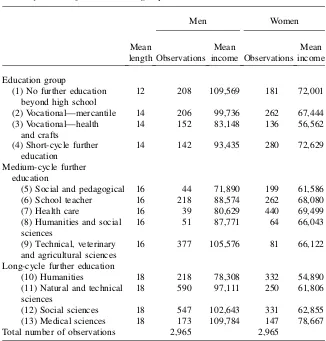
Now we go through the definition of educational groups in detail. The first group consists of those individuals who do not enroll in an education after high school. The remaining 12 groups then consist of individuals who enroll in one of the following educations: vocational education and training, short-cycle higher education, me-dium-cycle higher education, and long-cycle higher education. Individuals who en-roll in vocational education and training are subdivided into two groups where one consists of the mercantile educations, such as sales assistants, and the other consists of both crafts, such as electricians or plumbers, and health or pedagogical educations, for example, orthopedists. The short-cycle higher educations are all grouped together and are subject-wise more diverse than the other groups. Examples of short-cycle higher educations are real estate agents and various forms of technicians.
Individuals who enroll in medium-cycle higher educations are subdivided into five groups. The first group consists of pedagogical educations, such as nursery teachers and social workers. The second group comprises school teachers at the basic and lower secondary level. The third group consists of educations that lead to jobs in the public health system, for example, nurses and physical therapists. The fourth group consists of educational subjects within the range of humanities and business, for example, journalists, librarians, and graduate diplomas in business administra-tion. The final group comprises technical, veterinary, agricultural, and military edu-cations, for example, engineers.
Finally, individuals who enroll in long-cycle higher educations are divided into four groups: the humanities, the natural and technical sciences, the social sciences, and the medical sciences. These are university educations. In Table 2, the distribution of males and females across educational groups are presented together with informa-tion on mean income levels.
From Table 2, we see that women are overrepresented in educational groups that contain social and pedagogical and health care elements, whereas men are more in-clined to take an education in natural sciences, technical, veterinary, and agricultural sciences, and social sciences. Table 2 also reveals that the mean level of income varies greatly across the 13 different age groups.
Table 3 reports the ratio of actual to expected frequency of a given educational combination to show the educational combinations of couples. The expected fre-quency is the number of couples in a given cell had the matching been random by education.4 For instance, for couples in medical sciences (Combination 13-13, see Table 2), the expected frequency would be 8.58 (147*173/2,965), whereas the actual frequency is 33 couples; this makes up a ratio of 3.85 (33/8.58). Ratios above one are highlighted, and they represent educational combinations that are more common than would be the case under random matching by education.
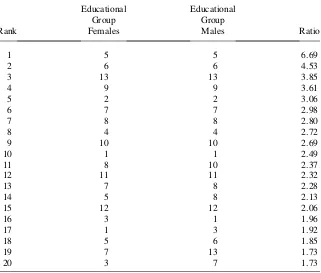
A pattern of positive assortative matching on education shows up. All couples with the same education (that is, at the diagonal) are systematically more common.5 How-ever, there are large differences between the tendency toward homogamous marriage. In Appendix A, Table A1, we show the ranking of couples by ratio. The top three couples are social and pedagogical couples, teacher couples, and medical science couples. The first ten places on the ranking are occupied by couples with the same educations. Among the couples that do not consist of people with similar educational attainment, the more popular are, as expected—female nurses who hook up with male medical doctors (Rank 19).
The empirical analysis that follows is going to shed more light on the reasons for positive assortative matching and other systematic matching patterns on education. The next two subsections present the variables needed to test whether partnership formation happens due to preferences or opportunities or both. First, we define
Table 1
Sample selection
Number of observations
Sample of individuals born 1955–65 26,048
Who completed at least high school 6,946
Relationships formed between 1980–95 19,938
Where both partners completed high school 3,144
Relationships where information on institution and municipality of education is available for both partners
2,965
4. Note that the expected frequencies are calculated based on the numbers in Table 2 and not on the mar-ginal distributions for all of Denmark.
5. Couples on the diagonal make up 22 percent of all couples, whereas couples with the same length of education amount to 43 percent of all couples in our sample.
variables that describe the couples’ income processes. Second, we present variables that measure the search costs for matching with a specific educational type.
1. Income measures
To assess whether a given portfolio of two educations fulfills the requirement of be-ing a good economic match, we calculate a number of simple income measures based on the time-series variation in incomes between different educational groups. We base the income measures on income information for all individuals sampled over educational groupings instead of just using data from observed partnerships. The lat-ter suffers from potential endogeneity bias (see, for example, Hess 2004). Along the
Table 2
(2) Vocational—mercantile 14 206 99,736 262 67,444
(3) Vocational—health
(5) Social and pedagogical 16 44 71,890 199 61,586
(6) School teacher 16 218 88,574 262 68,080
(7) Health care 16 39 80,629 440 69,499
(8) Humanities and social
(10) Humanities 18 218 78,308 332 54,890
(11) Natural and technical sciences
18 590 97,111 250 61,806
(12) Social sciences 18 547 102,643 331 62,855
(13) Medical sciences 18 173 109,784 147 78,667
Total number of observations 2,965 2,965
Table 3
Ratios of actual to expected frequency
Males Females
1 2 3 4 5 6 7 8 9 10 11 12 13
1 2.49 1.47 1.96 0.88 1.08 0.72 1.00 0.50 0.93 0.65 0.39 0.53 0.59
2 1.69 3.06 0.82 1.12 0.79 0.67 0.60 0.35 0.42 0.51 0.45 0.79 0.61
3 1.92 1.07 1.32 1.36 1.42 0.83 0.94 1.56 0.25 1.16 0.40 0.43 0.55
4 1.54 1.13 1.39 2.72 0.96 0.71 0.90 0.00 1.05 0.51 0.51 0.58 0.43
5 0.32 0.66 0.51 0.50 6.69 1.30 1.09 0.00 0.00 1.27 0.00 0.00 0.00
6 0.38 0.26 0.52 0.70 1.85 4.53 0.91 1.31 0.52 0.55 0.28 0.56 0.58
7 0.00 0.49 1.73 0.28 0.00 0.88 2.98 1.22 0.97 0.72 0.63 1.44 0.00
8 0.55 0.38 0.44 0.43 2.13 0.23 2.28 2.80 0.74 1.28 0.96 0.74 0.00
9 0.83 1.34 0.93 0.93 0.80 0.74 1.30 0.74 3.61 0.79 0.82 0.65 0.76
10 0.63 0.17 1.02 0.55 0.98 1.04 0.68 2.37 0.17 2.69 1.00 1.02 1.14
11 0.49 0.64 0.98 1.06 0.60 0.77 0.90 0.88 1.14 1.03 2.32 1.04 1.26
12 0.96 0.74 0.93 0.93 0.81 0.72 0.80 1.20 0.27 1.12 0.91 2.06 1.02
13 0.24 0.44 0.26 0.82 0.71 0.33 1.73 1.10 0.65 0.91 1.20 0.97 3.85
Note: Bold indicates that the actual frequency is higher than the expected frequency.
Nielsen
and
Sv
arer
lines of Hess (2004), we present three narrowly defined income measures: income correlation, relative volatilities, and mean difference to describe the income pro-cesses in relationships within different educational groupings. In addition, we sum-marize the characteristics of the income processes of two partners given educations by the standardized return.
To construct the income measures we use data for all years (1980-95) for all indi-viduals with at least a high school degree. We base the income measures on residuals from two gender-specific Mincer wage regressions of log net income on experience and experience squared.6
Based on the residuals for men and women, we compute the correlation between partners’ income residuals as a pooled time-series correlation. More specifically, for a man in educational groupiand a woman in educational groupj, the correlation is defined as the correlation over time between the mean income residuals of men in educational group i and women in educational group j. All income measures are per definition the same for any couple with the same educational combination. Sim-ilarly, the income gap is defined as jYiYjj and the variance gap is defined as max sj
si; si sj
, where Yi=Yj are the mean income residuals for groupsiandj, and
sj,siare the standard deviation of the mean income residuals for groupsiandj. The standardized return is computed as the sum of the mean residuals for a couple divided by the standard deviation on the sum of residuals. Due to the similarity with the return to a financial portfolio, we denote the standardized return the ‘‘Sharpe’’ ratio. That is, for a man in educational group iand a woman in educational group
j, the Sharpe ratio is the sum of the mean income residual for groupsiandjdivided by the standard deviation of the sum of the two mean income residuals. This ratio measures the mean income residual per unit of variability, meaning that this measure indicates how good the partnership between two individuals is in terms of generating a certain income level.
In terms of defining a good portfolio of educations in marriage, individuals should seek to form partnership with individuals who have education that gives a high mean, low variance, and a negative correlation. Focusing on the summary measure, individ-uals should seek partners with a high Sharpe ratio. In Table 4, we report the estimated correlation and Sharpe ratios for the 13*13 educational mating possibilities. Looking across the diagonal elements, we see positive correlations for 11 out of 13 educational groupings. Also, the Sharpe ratios are relatively modest (except for couples where both studied medical science after high school and couples where both have mercantile vo-cational training). This pattern tentatively suggests that finding a good economic match is not the main determinant for observed partnership formation.
2. Distance Measures
To investigate how search costs affect marriage market behavior, we include a variety of distance measures between educational groups in the analysis. The basic
Table 4
Correlation (top figure) and Sharpe ratios (bottom figure) for pairs of educational groups
Males Females
1 2 3 4 5 6 7 8 9 10 11 12 13
1 0.851 0.740 0.683 0.679 0.344 20.557 0.753 0.663 20.515 20.219 0.661 20.767 20.278
0.126 0.430 20.279 20.107 0.158 20.212 0.267 0.048 20.302 20.571 0.085 0.077 0.576
2 0.928 0.886 0.616 0.811 0.213 20.230 0.834 0.708 20.495 20.169 0.784 20.415 20.304
0.345 0.676 2.069 0.190 0.589 0.287 0.527 0.312 0.104 20.009 0.391 0.584 1.181
3 0.665 0.665 0.419 0.462 20.028 20.248 0.716 0.366 20.461 20.152 0.704 20.130 20.135 20.418 20.181 20.858 20.937 20.981 21.281 20.363 20.649 21.163 22.151 20.690 21.030 20.763
4 0.973 0.935 0.652 0.850 0.257 20.351 0.882 0.756 20.480 20.095 0.742 20.460 20.214 20.084 0.159 20.477 20.370 20.223 20.629 0.008 20.197 20.672 20.998 20.209 20.468 0.023
5 0.142 0.153 0.205 0.008 0.160 20.005 0.250 0.298 20.007 0.659 0.315 0.198 0.491 20.148 0.050 20.462 20.383 20.214 20.386 20.070 20.222 20.426 20.498 20.223 20.268 20.074
6 0.267 0.265 0.001 0.147 0.276 0.461 0.155 0.282 0.161 20.350 0.396 0.218 20.562
0.173 0.588 20.366 20.147 0.214 20.135 0.382 0.068 20.227 20.853 0.119 0.047 1.021
7 20.135 20.069 0.148 20.070 20.348 20.079 0.048 20.023 20.103 0.733 20.077 0.336 0.737 20.651 20.439 20.875 20.923 20.857 20.929 20.550 20.739 20.933 20.971 20.787 20.717 20.529
8 20.328 20.258 20.491 20.389 20.024 0.316 20.406 20.081 0.637 0.491 20.370 0.245 0.354 20.115 0.246 20.741 20.551 20.200 20.380 0.030 20.233 20.359 20.670 20.285 20.259 0.030
9 20.006 20.022 20.060 20.006 0.212 0.754 20.163 0.197 0.280 20.029 0.225 0.414 20.401
0.160 0.577 20.375 20.164 0.160 20.126 0.380 0.045 20.219 20.593 0.089 0.018 0.664
10 20.277 20.190 20.530 20.234 0.165 0.860 20.428 20.023 0.680 20.087 20.209 0.589 20.296 20.315 0.042 20.974 20.839 20.474 20.542 20.230 20.454 20.538 21.348 20.572 20.458 20.288
11 0.205 0.275 0.066 0.325 0.035 0.681 0.155 0.507 0.214 0.284 0.215 0.578 0.067 0.167 0.575 20.367 20.150 0.221 20.137 0.371 0.055 20.232 20.623 0.114 0.031 0.635
12 0.498 0.513 0.180 0.555 0.514 0.387 0.332 0.725 0.243 0.161 0.335 0.145 20.205
0.047 0.419 20.467 20.298 20.001 20.317 0.218 20.069 20.356 20.960 20.058 20.145 0.475
13 0.259 0.452 20.017 0.094 0.440 0.136 0.173 0.296 0.375 0.473 20.139 0.130 0.031
0.380 0.754 20.147 0.175 0.507 0.169 0.622 0.310 0.012 20.111 0.506 0.366 0.998
Note: Bold indicates that the actual frequency is higher than the expected frequency.
Nielsen
and
Sv
arer
idea is that educations that are closer to each other, as measured by the physical distance between the institutions at which the particular education is started, should generate more intra-educational matching since it is cheaper to locate a suitable partner.
Two different measures of distance between the partners are used. The first mea-sure is the density (density) of women in educational groupjin the man’s municipal-ity of education in the year he enrolls in the education. The second is an indicator of whether or not the spouses have attained their education at the same educational in-stitution (same institution).
In calculating the first distance measure, we use all educational information avail-able, not only on the individuals in the 2,965 couples, but on all high school gradu-ates in the sample. On the basis of this educational information, we determine the density as a measure of the concentration of different educational groups in the mu-nicipalities. It measures the density of individuals from a specific educational group in a specific municipality. For a man who has taken his education in municipalitym
and who enrolled in year t, and whose partner belongs to educational groupi, the density is defined as the proportion of women in municipality mfrom educational groupiin yeart.
Descriptive statistics for the distance measures are presented in Table 5 for the part-nership formation analysis. The distance measures are proxies for search cost of finding a partner with a given level of education since we do not know if a given partnership is formed because the couple met in school. It could also be the case that the reason we find substantial homogamy in terms of education is that people with similar types of educa-tion have the same workplaces after graduaeduca-tion. After school, the workplace is the most likely place to meet a marriage partner according to both Laumann et al. (1994) and Kalmijn and Flap (2001). We address the latter issue in the following section where we perform a multivariate analysis of partnership formation.
III. Empirical Analysis
Below, we investigate how economic conditions and accessibility of partners are associated with partnership formation. The question we try to answer is: Do positive assortative matching in education persist when we control for proximity of partners and economic factors?
To answer this, we follow the empirical strategy of Dalmia and Lawrence (2001) and Jepsen and Jepsen (2002). They both use conditional logit models to compare actual couples with randomly created couples to see if actual couples are more sim-ilar or more different than the random pairings.
The empirical procedure works as follows: In the first step, the relevant explana-tory variables are defined. In this application we include: age difference between partners, an indicator for whether they attend the same education, characteristics of the income residuals for the educational grouping of partners, distance measures between partners’ educational institutions, an indicator variable for whether the part-ner attended the same educational institution, and a density measure of the partpart-nersÕ
of available partners to a given person (we do not construct same sex couples).7The final step is to predict the sign of the coefficients based on the level of positive or negative assortative matching. The conditional logit model is:
PðYi¼jÞ ¼
exijb +exijb; ð1Þ
whereiis an individual,jis an alternative, andxijis the vector of characteristics of the couple created by matching personiwith an alternativej. Letting the dependent variable take the value one for a natural couple and 0 for an artificial couple, we ex-pect to find a negative coefficient to the age difference, since positive assortative matching means that the age difference should be smaller for actual couples than for artificial couples. Likewise, if a couple is more likely to form if the partners at-tend the same educational institution, the coefficient tosame institution should be positive. We assume in the following that the explanatory variables are exogenous to the partnership formation process.8
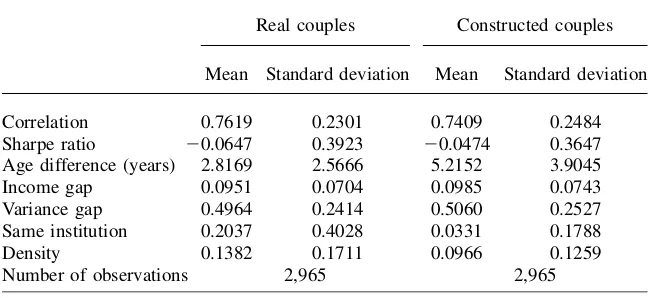
In Table 5, we present descriptive statistics for the information used in the match-ing analysis.
Table 5
Descriptive statistics for variables used in matching analysis
Real couples Constructed couples
Mean Standard deviation Mean Standard deviation
Correlation 0.7619 0.2301 0.7409 0.2484
Sharpe ratio 20.0647 0.3923 20.0474 0.3647
Age difference (years) 2.8169 2.5666 5.2152 3.9045
Income gap 0.0951 0.0704 0.0985 0.0743
Variance gap 0.4964 0.2414 0.5060 0.2527
Same institution 0.2037 0.4028 0.0331 0.1788
Density 0.1382 0.1711 0.0966 0.1259
Number of observations 2,965 2,965
7. We only construct one artificial match for each couple. Jepsen and Jepsen (2002) also used 1, but state that sensitivity analysis where three artificial partners were constructed did not alter their results. In addi-tion, McFadden (1973) shows that the conditional logit model produces consistent parameter estimates when a random subset of nonchosen alternatives is used.
8. Our empirical strategy has the advantage that it allows us to include a range of explanatory variables in the description of the matching pattern in the marriage market. The downside is that we basically treat a two-sided matching situation as one-sided. That is, the model we use characterizes the rational behavior of an agent that chooses between different options. In the marriage market context the preferred option has the possibility to reject. Preferably, the empirical model should compare the chosen partner to every possible partner available in the market. Since we have no data on all possible partners in the marriage mar-ket and no clear model of the value of marriage conditional on each possible choice, we choose to follow the outlined strategy, although we acknowledge that it simplifies the analysis and hence that the results we find must be interpreted accordingly.
The first columns show the mean and standard deviation for the explanatory var-iables for the 2,965 couples in the sample. Around 20 percent of the couples attended the same educational institution. This does not necessarily imply that they met at the time of education, but it strongly suggests that educational institutions do provide fa-cilities for partnership search.9
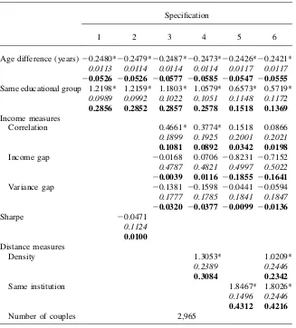
Table 6 presents the results from the conditional logit model for partnership for-mation. In all specifications, we find that a lower age difference between two indi-viduals is associated with a higher probability that they form a partnership. This pattern is as expected and in accordance with the marriage formation literature that finds strong positive assortative mating in age.
In the first specification, we add to the age difference an indicator for whether the partners have the same education. We find that when choosing among two otherwise identical partners, the probability of choosing the one with the same education as ones own is 29 percentage points higher. This conforms to the patterns of positive assortative matching on education, which we saw in the previous subsection and which is well known in the literature. The estimated marginal effect is unaffected by including income-related variables (Specifications 2 and 3). However, it is ap-proximately halved when proximity of partners is controlled for in particular through the dummy variable for same institution (Specifications 4 to 6). Hence, roughly half of the educational sorting is adirect effectof the partners’ education that is unrelated to educational institutions.
We interpret the half of educational sorting that is unrelated to educational insti-tutions as potentially related to complementarities in household production. It may be viewed as a lower bound on the effect because one could imagine some comple-mentarities in household production that are related to the educational institution (for example, preferences for the same sporting events, shared value systems, or identical preferences for certain pedagogical approaches) or the geographical areas around the educational institution (for example, family attachment or preferences for the local area). Using data from Denmark, we are confident that these examples are of minor importance. In contrast to the United States, sporting events and sports activities are not an integrated part of college life in Denmark, and they play no role whatsoever in the recruiting of students. Therefore, preferences for such activities do not flaw the interpretation as it would have done for the United States. Although traveling time between the major cities rarely exceeds three hours, the population is sometimes regarded as immobile. This could be a potential obstacle to our interpretation of ‘‘same institution’’ as an indication of low search frictions. However, statistics from, for example, University of Aarhus (Aarhus University 2000) reveals that less than half of the applicants came from the two neighbor counties, and only a quarter of the applicants report that geographical placement was important for their application to the university. We cautiously conclude that issues of complementarities in house-hold production are of minor importance in the interpretation of the proximity variables. If, however, the proximity variables reflect household complementarities as well as search costs, the inclusion of proximity indicators should be viewed as a selection correction for selection into same education assuming linear selection on
observables. In this case it would be inappropriate to interpret the coefficients to the proximity variables as indicative of search frictions. On the other hand, there may also be lower search frictions for partners with same education in other marriage markets, for instance, at the workplace since there is an increased probability of em-ployment in the same company if the partners have the same education. We return to this situation in Table 7, where we present results for two different samples. One where we discard couples who had the same workplace prior to relationship start and one where we discard couples who attended the same high school.
Table 6
Results for partnership formation analysis
Specification
1 2 3 4 5 6
Age difference (years)20.2480*20.2479*20.2487*20.2473*20.2426*20.2421*
0.0113 0.0114 0.0114 0.0114 0.0117 0.0117
20.0526 20.0526 20.0577 20.0585 20.0547 20.0555
Same educational group 1.2198* 1.2159* 1.1803* 1.0579* 0.6573* 0.5719*
0.0989 0.0992 0.1022 0.1051 0.1148 0.1172
0.2856 0.2852 0.2857 0.2578 0.1518 0.1369
Income measures
Correlation 0.4661* 0.3774* 0.1518 0.0866
0.1899 0.1925 0.2001 0.2021
0.1081 0.0892 0.0342 0.0198
Income gap 20.0168 0.0706 20.8231 20.7152
0.4787 0.4821 0.4997 0.5022
20.0039 0.0116 20.1855 20.1641
Variance gap 20.1381 20.1598 20.0441 20.0594
0.1777 0.1785 0.1841 0.1847
20.0320 20.0377 20.0099 20.0136
Sharpe 20.0471
0.1124
0.0100
Distance measures
Density 1.3053* 1.0209*
0.2389 0.2446
0.3084 0.2342
Same institution 1.8467* 1.8026*
0.1496 0.2446
0.4312 0.4216
Number of couples 2,965
Note: For each variable we present the estimated coefficients, the standard errors (in italics), and the mar-ginal effects (in bold). * indicates significance at (at least) the 5 percent level.
In the second and third specifications (in Table 6), we include only income-related variables. The more correlated the income residuals for the educational groups are, the more likely is it that a match is made, which most likely indicates omitted vari-able bias. Also, the possibility of forming a partnership with a person with whom it is possible to construct a high yield return corrected for variability does not seem to drive partnership formation either. These findings could suggest that either individ-uals do not pay attention to these considerations when they form partnerships, or that they simply do not have sufficient information to judge whether a potential partner offers a good hedge and a high variance-corrected return. Alternatively, it may be a consequence of the generous welfare state that equalizes incomes over time and over individuals.10
In Specifications 4 to 6, we include variables capturing the proximity of partners. We find that the effect from income correlation becomes insignificant at conventional levels of significance.11
So the finding that individuals with higher positively correlated income processes are more likely to marry seems to follow from their closer proximity while undertak-ing education. This conjecture is consistent with the findundertak-ing that the included prox-imity variables all have a significant influence on partnership formation and that the effects are working in the expected direction. That is, an individual is more likely to form partnership with a person who, after high school, attends the same educational institution (for example, the same university or the same business school). The mar-ginal effect of the indicator variable is rather high, indicating that the probability for a match is raised by 43 percentage points if two persons share educational institu-tion.12Also, we find that a higher density of partners with a given education is as-sociated with an increased propensity that an individual forms partnership with a person with this educational attainment.
Table 7 presents results for three slightly adjusted samples as robustness checks. In the first set of columns we exclude couples who meet before college. In this speci-fication, the effect of the income gap becomes significant. This may be interpreted as evidence that the marriages that are formed before college are more for ‘‘love,’’ while for the later ones income play a more important role.13In the second set of columns we exclude couples that worked at the same workplace the year before mar-riage (about 5 percent of the couples), and we find that the marginal effect of same education is reduced from 26.6 to 8.5 percentage points when we include proximity variables. Hence, a small part of assortative matching on education is related to the fact that people with the same educations are more likely to share workplace than others. In the third set of columns we exclude couples that attended the same high school (about 20 percent of the couples), and we find that the marginal effect of same education is reduced from 28.3 to 12.3 percentage points when we include proximity
10. We also tried to include the difference in mean unemployment degrees in the partners’ educational groups. This variable is not significant either, which is consistent with the generous welfare state hypothesis. 11. As a robustness check, we have computed the income variables based on the five-year periods follow-ing partnership formation (for example, for couples formed in 1981, we use 1981-86). This may be a better reflection of what couples expect at the time of marriage. This refinement leaves the results unchanged. 12. Strictly speaking, they do not have to meet each other at the institution since there are no time limi-tations to when they enrolled and graduated.
Table 7
Results for partnership formation analysis, sensitivity checks
Specification
Only couples who prior to the relationship were: Exclude couples who
meet before college not at the same workplace not at the same high school
Age difference (years) 20.267* 20.255* 20.267* -0.264* 20.2183* 20.216*
0.014 0.014 0.012 0.012 0.0121 0.012
20.056 20.055 20.054 -0.061 20.0483 20.051
Same educational group 1.234* 0.561* 1.161* 0.358* 1.1972* 0.506*
0.105 0.125 0.101 0.125 0.1071 0.128
0.286 0.129 0.266 0.085 0.2854 0.123
Income measures correlation 0.227 0.447* 0.165
0.222 0.216 0.220
0.049 0.104 0.039
Income gap 21.695* 20.520 20.544
0.561 0.525 0.538
20.369 20.121 20.129
Variance gap 20.321 20.351 20.150
0.209 0.200 0.205
20.069 20.082 20.035
(continued)
Nielsen
and
Sv
arer
Table 7 (continued)
Specification
Only couples who prior to the relationship were: Exclude couples who
meet before college not at the same workplace not at the same high school
Distance measures
Density 0.481* 0.917* 0.796*
0.253 0.254 0.2583
0.104 0.213 0.1888
Same institution 1.925* 2.486* 2.0683*
0.169 0.201 0.1819
0.447 0.534 0.4657
Number of couples 2,392 2,804 2,390
Note: For each variable, we present the estimated coefficients, the standard errors (in italics) and the marginal effect (in bold). * indicates significance at (at least) the 5 percent level.
The
Journal
of
Human
variables. The robustness checks in Table 7 indicate that workplaces and high schools also are marriage markets that promote matching of individuals with same education and thus are relevant for the analysis of how much of educational homog-amy stems from opportunities to meet.14To sum up, even less educational homog-amy is left unexplained (40 percent instead of 50 percent), when we deduct people who potentially met in high school or at their workplace.
An additional consideration is relevant in relation to the couples who attended the same high school. If they already started to date at this time and subsequently coor-dinated their choices of where to pursue further education, the distance measures might be endogenous to the partnership formation process (at least for those who continued the relationship after they started further education). If endogeneity were a major concern, we would expect that the coefficients to the distance variables were biased away from zero.
Compared to the results in Table 6, the density and same institution variables show a somewhat smaller effect in Table 7, but the change is very modest. Consequently, we do not think that the inclusion of individuals who attended the same high school is a major problem, and we rely on Table 6 for the main conclusion of this part of the paper.
As an additional robustness check, we have estimated the conditional logit model with indicator variables for educational cross-terms of couples.15First, we estimate the conditional logit model with 13*13 cell indicators, and then we test down. This procedure leaves us with 17 indicators for education cells. As before, we find a clear positive assortative matching on education and, as before, we find that including in-come-related variables leaves the coefficients literally unaffected. When we control for proximity of partners, we see that more than half of the indicators referring to diagonal cells go down and become insignificant. This analysis allows us to name some couples who seem to appreciate the same public goods—that is, couples with a vocational mercantile education (2-2), couples with further education in the hu-manities (10-10), couples with further education in medical sciences (13-13), and nurses and medical doctors (7-13).
All in all, the partnership formation analysis suggests that search costs are indeed important for partnership formation and that individuals apparently search in mar-riage markets that are close to the place where they attend school. A main conclusion from this matching analysis is that we find a clear pattern of assortative matching on education, and half of that stems from low search costs for partners at the educational institutions. Another important conclusion is that we find no evidence suggesting that economic conditions are important.
IV. Concluding Remarks
In this paper, we take a closer look at the observation that individuals tend to match on length and type of education. We investigate whether the systematic relationship between the educations of the partners is explained by opportunities, for
14. See, for example, Svarer (2007) for an analysis of workplaces as marriage markets.
15. To save space these results are not tabulated in the paper, please consult the working paper version for details, see Nielsen and Svarer (2006).
example, proximity to potential partners, or preferences, for example, complementar-ities in household production or portfolio optimization. We find that around half of the systematic sorting on education is related to the proximity of partners’ educa-tional institutions, whereas the income properties of the joint income process show no influence on partner selection. Thus, around half of the systematic sorting on ed-ucation represents a residual which may potentially be attributed to complementar-ities in household production.
For future research it could be fruitful to develop a theoretical justification of the empirical results presented in this paper. Hess (2004) provides a model that is con-sistent with some of the findings we present, but it does not address the issue of prox-imity of partners which constitutes one of the main mechanisms for partnership formation. In addition, the current analysis would benefit from some exogenous var-iation in the sex ratios at the different educational institutions that would affect the probability of finding a suitable partner close by.
Table A1
The 20 educational combinations with the highest ratio of actual to expected frequency
Educational Group
Educational Group
Rank Females Males Ratio
1 5 5 6.69
2 6 6 4.53
3 13 13 3.85
4 9 9 3.61
5 2 2 3.06
6 7 7 2.98
7 8 8 2.80
8 4 4 2.72
9 10 10 2.69
10 1 1 2.49
11 8 10 2.37
12 11 11 2.32
13 7 8 2.28
14 5 8 2.13
15 12 12 2.06
16 3 1 1.96
17 1 3 1.92
18 5 6 1.85
19 7 13 1.73
References
Aarhus University. 2000).‘‘Den Bla˚ A˚ rgang.’’ In Danish. Report.
Aiyagari, S. Rao, Jeremy Greenwood, and Nezih Guner. 2000. ‘‘On the State of the Union.’’ Journal of Political Economy108(2):213–44.
Barro, Robert J., and Jong-Wha Lee. 2001. ‘‘International Data on Educational Attainment: Updates and Implications.’’Oxford Economic Papers53(3):541–63.
Becker, Gary 1973. ‘‘A Theory of Marriage: Part I.’’Journal of Political Economy82(4):813– 46.
Becker, Gary, and Kevin Murphy. 2000.Social Economics: Market Behavior in a Social Environment.Harvard University Press.
Blau, Peter M., and Otis D. Duncan. 1967.The American Occupational Structure.John Wiley and Sons.
Brien, Michael, Lee Lillard, and Steven Stern. 2006. ‘‘Cohabitation, Marriage, and Divorce in a Model of Match Quality.’’International Economic Review47(2):451–94.
Boulier, Bryan L., and Mark Rosenzweig. 1984. ‘‘Schooling, Search, and Spouse Selection: Testing Economic Theories of Marriage and Household Behavior.’’Journal of Political Economy92(4):712–32.
Chen, Kong-Pin, Shin-Hwan Chiang, and Siu Fai Leung. 2003. ‘‘Migration, Family, and Risk Diversification.’’Journal of Labor Economics21(2):353–79.
Chiappori, Pierre-Andre., Murat Iyigun, and Yoram Weiss. 2006. ‘‘Investment in Schooling and the Marriage Market.’’ Unpublished.
Dalmia, Sonia, and Pareena G. Lawrence. 2001. ‘‘An Empirical Analysis of Assortative Mating in India and the U. S.’’International Advances of Economic Research7(4):443–58. Epstein, Elizabeth, and Ruth Guttman. 1984. ‘‘Mate Selection in Man: Evidence, Theory, and
Outcome.’’Social Biology31(4):243–78.
Fernandez, Rachel, and Richard Rogerson. 2001. ‘‘Sorting and Long-Run Inequality.’’ Quarterly Journal of Economics116(4):1305–41.
Fernandez, Rachel, Nezih Guner, and John Knowles. 2005. ‘‘Love or Money: A Theoretical and Empirical Analysis of Household Sorting and Inequality.’’Quarterly Journal of Economics120(1):273–44.
Gautier, Pieter A., Michael Svarer, and Coen N. Teulings. 2005. ‘‘Marriage and the City.’’ Working Paper 2005-01. Department of Economics, Aarhus University.
Goldin, Claudia. 1992. ‘‘The Meaning of College in the Lives of American Women: The Past One-Hundred Years.’’ NBER Working Paper No. 4099.
Halpin, Brendan, and Tak-Wing Chan. 2003. ‘‘Educational Homogamy in Ireland and the UK: Trends and Patterns.’’British Journal of Sociology54(4):473–95.
Hess, Gregory. 2004. ‘‘Marriage and Consumption Insurance: What’s Love Got to Do with it?’’Journal of Political Economy112(2):290–318.
Jepsen, Lisa K., and Christopher A. Jepsen. 2002. ‘‘An Empirical Analysis of the Matching Patterns of Same-Sex and Opposite-Sex Couples.’’Demography39(3):435–53.
Kalmijn, Matthijs, and Hendrik Flap. 2001. ‘‘Assortative Meeting and Mating: Unintended Consequences of Organized Settings for Partner Choices.’’Social Forces79(4):1289–1312. Kotlikof, Lawrence, and Avia Spivak. 1981. ‘‘The Family as an Incomplete Annuity Market.’’
Journal of Political Economy89:372–91.
Laumann, Edward, John Gagon, Robert Michael, and Stuart Michaels. 1994. ‘‘The Social Organization of Sexuality: Sexual Practices in the U. S.’’ Chicago: University of Chicago Press.
Lewis, Susan K., and Valerie K. Oppenheimer. 2000. ‘‘Educational Assortative Mating across Marriage Markets: Non-Hispanic Whites in the US.’’Demography37(1):29–40.
Mare, Robert D. 1991. ‘‘Five Decades of Educational Assortative Mating.’’American Sociological Review56:15–32.
McFadden. Daniel. 1973. ‘‘Conditional Logit Analysis of Qualitative Choice Behavior.’’ In Frontiers in Economics, ed. P. Zaremba. New York: Academic Press.
Micevska, Maja. 2002. ‘‘Marriage, Uncertainty, and Risk Aversion in Russia.’’ Draft. Center for Development Research. University of Bonn.
Nielsen, Helena S., and Michael Svarer. 2006. ‘‘Educational Homogamy: Preferences or Opportunities?’’ IZA DP 2271.
Rosenzweig, Mark, and Oded Stark. 1989. ‘‘Consumption Smoothing, Migration, and Marriage: Evidence from Rural India.’’Journal of Political Economy97:905–26. Schafer, Robert B., and Pat M Keith. 1990. ‘‘Matching by Weight in Married Couples: A Life
Cycle Perspective.’’Journal of Social Psychology130(5):657–64.
Scott, John F. 1965. ‘‘The American College Sorority: The Role in Class and Ethnic Endogamy.’’American Sociological Review30(3):514–27.
Svarer, Michael. 2007. ‘‘Working Late: Do Workplace Sex Ratios Affect Partnership Formation and Dissolution?’’Journal of Human Resources42(3):583–95.