The Role of Permanent Income and
Demographics in Black/White
Differences in Wealth
Joseph G. Altonji
Ulrich Doraszelski
A B S T R A C T
We explore the extent to which the large race gap in wealth can be explained with properly constructed income and demographic variables. In some instances we explain the entire wealth gap with income and demo-graphics, provided that we estimate the wealth model on a sample of whites. However, we typically explain a much smaller fraction when we estimate the wealth model on a black sample. Using sibling fixed-effects models to control for intergenerational transfers and the effects of adverse history, we find that these factors are not likely to account for the lower explanatory power of the black wealth models. Our analysis of growth mod-els of wealth suggests that differences in savings behavior and/or rates of return play an important role.
I. Introduction
The wealth gap between whites and blacks in the United States is much larger than the gap in earnings (see, for example, Menchik and Jianakoplos 1997). The gap in wealth has implications for the social position of African
Joseph G. Altonji is a professor of economics at Yale University and a research associate at NBER. Ulrich Doraszelski is an assistant professor of economics at Harvard University. The authors thank Ken Housinger for assisting with the data. They also thank Michaela Draganska, William Gale, Bruce Meyer, two anonymous referees, and seminar participants at the Federal Reserve Bank of Chicago (May 1999), Northwestern University (December 2000), the University of Wisconsin (June 2001), and Yale University (December 2002) for helpful comments. They are grateful for support from the Federal Reserve Bank of Chicago, the Russell Sage Foundation, and the Institute for Policy Research at Northwestern University. The authors owe a special debt to Lewis Segal who collaborated with them in the early stages of the proj-ect. A less technical, abbreviated summary of some of the research reported here may be found in Altonji, Doraszelski and Segal (2000). All opinions and errors are our own. The data used in this article can be obtained beginning October 2005 through September 2008 from the authors at these addresses: Altonji, Box 208269, New Haven, CT 06520-8269, U.S.A., joseph.altonji@yale.edu, doraszelski@harvard.edu [Submitted October 2001; accepted September 2003]
Americans that go far beyond its obvious implications for the consumption levels that households can sustain. This is because wealth is a source of political and social power, influences access to capital for new businesses, and provides insurance against fluctuations in labor market income. It affects the quality of housing, neighborhoods, and schools a family has access to as well as the ability to finance higher education. The fact that friendships and family ties tend to be within racial groups amplifies the effect of the wealth gap on the financial, social, and political resources available to blacks relative to whites.
The first question we ask in this paper is: To what extent can the large race gap in wealth be explained with income and demographic variables? Several previous studies (see Scholz and Levine 2002) for an up-to-date survey of the literature) have investigated the sources of the black/white wealth gap. We improve on these studies in a number of ways. First, the existing studies do not use an adequate measure of permanent income, which is a key determinant of wealth. Due to data limitations Smith (1995) and Avery and Rendall (1997) base their wealth models on current income alone rather than on current and permanent income. Blau and Graham (1990) and Menchik and Jianakoplos (1997) decompose income into cur-rent income and permanent income, where permanent income is the component that is predictable given race, sex, age, education, health status, number of chil-dren, and geographic location. Since wealth is a nonlinear function of income, however, use of the within-cell variation is necessary to precisely estimate wealth models. Moreover, because high-income individuals tend to have disproportion-ately large wealth holdings, failure to accurdisproportion-ately measure the tails of the distribu-tion of permanent income might lead to incorrect estimates of the contribudistribu-tion of permanent income to the wealth gap. We address this issue by using panel data from the Panel Study of Income Dynamics (PSID) to construct a measure of per-manent income. Second, previous studies control for current demographic vari-ables such as marital status and presence of children but not for demographic histories which should influence current wealth through past savings. We address this by constructing marriage histories and child-bearing and -rearing histories. Third, to account for the fact that wealth is frequently zero or negative and has a highly skewed distribution and that demographic variables are likely to interact with income variables, we use both mean and median regression and work with models of the wealth/permanent income ratio as well as the level and log of wealth. A fourth problem arises from the substantial differences between the white and black distributions of income and demographics in combination with the fact that relatively flexible functional forms must be used to capture the nonlinearity of wealth in income (see also Barsky, Bound, Charles, and Lupton 2002). These two features make it difficult to accurately estimate race-specific wealth models over the full range of income. We address this “nonoverlap” problem in several ways and check that our main results are robust to it.
With our improved income and demographic variables, we typically explain more of the wealth gap than previous studies (Section IV). In the case of single men and single women, for example, we can explain the entirerace gap in the level of wealth with income and demographics provided that we estimate the wealth equation on the white sample. At the same time, we confirm earlier results that The Journal of Human Resources
suggest large disparities in the explanatory power of the wealth models of whites and blacks. While income and demographics account for 79 percent of the wealth gap in the case of couples when we use the wealth mean regression model for whites, we explain only 25 percent when we use the wealth model for blacks. When we use the ratio of wealth to permanent income as our measure of wealth, we again explain a much larger fraction of the wealth gap using the coefficients for whites than the ones for blacks, although for couples and single females the frac-tion explained is smaller than in the case of the level of wealth. Our results indi-cate that race differences in self-employment patterns are a significant part of a full explanation of black/white wealth differences, although causality is ambiguous. We also show, in contrast to the analysis of Barsky et al. (2002), that these findings are notdue to a lack of overlap between the white and black samples.
The fact that we can explain most and in some cases all of the wealth gap with the white but not with the black wealth model leads us to focus on a second question: Why are the wealth holdings of blacks less sensitive to income and demographics than the wealth holdings of whites? Starting with Blau and Graham (1990), some researchers have hypothesized that differences in inter vivos transfers and inheritances play a major part in explaining the wealth gap. In Section V, we propose a theoretical model of intergenerational linkages to show how the legacy of discrimination could lead to a link between wealth and income that is stronger for whites than for blacks. We study this possibility by relating differences among siblings in current and permanent income and demographics to differences in wealth. Using sibling comparisons largely neutralizes the effects of disparities between whites and blacks in inter vivos transfers and inheritances and provides a way of controlling for the effects of an adverse his-tory on the relative position of blacks. Our study is the first (to our knowledge) sib-ling fixed-effects analysis of wealth holdings and is of independent interest. With fixed-effects coefficient estimates from the white sample we can explain 104 percent of the race gap in the wealth level, while the corresponding value based on the model for blacks is only 49 percent. Our sibling results thus confirm that wealth holdings are much less strongly related to income and demographic variables among blacks than among whites. They are also consistent with evidence in Altonji and Villanueva (2001) based on both the PSID and the survey of Asset and Health Dynamics (AHEAD). This suggests that little of the difference between whites and blacks in the effect of income on wealth is due to differences in inter vivos transfers and inheri-tances.
Other explanations for the racial difference in the sensitivity of wealth holding to income and demographic variables are that savings rates or the rates of return to assets differ. In Section VI, we look at the combined effect of these two factors by estimat-ing models for the growth of wealth as a function of income and demographic factors. In the case of couples, income and demographic factors explain 74 percent of the race gap in the growth of wealth when we use the growth model for whites but only 49 per-cent when we use the growth model for blacks. The discrepancy is even larger (84 percent versus 30 percent) when we study growth in the ratio of wealth to per-manent income. These findings suggest that difference in savings behavior or rates of return on assets play a key role in explaining the wealth gap. However, the results are not entirely conclusive for reasons we discuss below.
II. Econometric Models and Wealth Decompositions
income variables (including current income yitand permanent income yi), and Xi ja
vector of demographic variables. Because we have panel data on wealth, a number of variables in addition to yitdepend on the calendar year tas well as i, but we leave the time subscript implicit.
Our basic wealth model specifies the level of wealth to be linear in the income and demographic variables and is given by
( )1 Wiw w Y X ,
ibare the corresponding parameters and error term for blacks. We define α0j+ Yi
jαj+ Xi
jβjto alternatively be the conditional mean
or the conditional median regression function. Separate sets of regressions are speci-fied for couples, single males, and single females, so the slopes and intercepts depend on sex and marital status as well as on race.
Given that the level of wealth is used as the dependent variable, Equations 1 and 2 impose additive separability between the income and demographic variables. We work with the levels of wealth because much of the public discussion is couched in terms of levels and because of the large fraction of the population with zero or neg-ative wealth. However, such level models imply that wealth is additively separable in income and demographic variables, which is unlikely. Consequently, we also work with the log of wealth and the ratio of wealth to permanent income of the household head as the dependent variable. The log model implicitly allows for mul-tiplicative interactions in the equation for the level of wealth. However, the log specification is poorly suited as a wealth model because wealth holdings are fre-quently close to zero or even negative. We deal with this problem by truncating these values prior to taking logs. The ratio specification avoids this problem alto-gether and implies that the effects of demographic variables are proportional to per-manent income.
Our choice of control variables is driven largely by previous studies of wealth dif-ferences, although our specifications of permanent income and marriage histories, and child-bearing and rearing histories are more elaborate. We chose to start with and stick to a fairly broad set of variables rather than “fish around” for a shorter list of variables that are statistically significant.
In the case of couples, the income controls included in Yi
jare current family nonasset
income, permanent income of the husband, permanent income of the wife, the squares of current income, head’s permanent income, and wife’s permanent income, as well as the products of current family income with the head’s and the wife’s permanent income. The income controls in the case of singles are similar except that spouse variables are excluded. For single men and women our demographic controls are region (four cate-gories), residence in a standard metropolitan statistical area, number of kids in the family unit, a dummy for whether there is at least one kid in the family The Journal of Human Resources
unit, the number of dependents outside the family unit and a dummy for whether there is at least one dependent outside the family unit, number of siblings, number of marriages, whether the most recent marriage ended in widowhood, whether the most recent marriage ended in divorce, the number of children born or adopted, and dummies for health status only poor or fair, education (six categories), self-employed, and the year of the wealth observation. In the case of couples we include health, education, self-employment, number of siblings, number of marriages, and number of children born or adopted measures for both the head and the spouse. We also include spouse’s annual hours worked. In addition, we include fourth-order polynomials in the age of the husband and in the age of the wife (centered at 40) in Xi
j. Because we estimate wealth models by demographic group, our age controls
implicitly account for group differences in life expectancy.
It is useful to discuss our choice of variables in light of economic theories of sav-ings and wealth (see Browning and Lusardi 1996 for a survey). The basic life cycle model of consumer behavior augmented to include a bequest motive suggests that wealth at a point in time will be influenced by the level and timing of earnings over the lifecycle, rates of time preference, rates of return, and consumption needs of the household. This suggests a role for both current and permanent earnings, powers of age, and various demographic variables that may influence the level and timing of consumption needs and perhaps are related to rates of time preference. Some of the variables we include, such as health status, are likely to operate through several of these channels.1We do not have direct measures of rates of return. Recent work
emphasizes precautionary savings and risk aversion, suggesting a role for measures of risk exposure and tolerance, insurance, and ability to borrow against future income. We do not have direct measures of these factors either. Some of the race dif-ferences in the effects of variables that we include may, however, be related to these factors.
We evaluate the explanatory power of our wealth models using a slightly modified regression decomposition (Blinder 1973, Oaxaca 1973) that allows for median regres-sion models and accommodates the use of population weights in computing the wealth gap. Let {ωi
j} i=1
Njdenote a set of population weights such that ω i
j> 0 and ∑ i=1
Nj
ωi
j= 1. (See Section III for details on how the weights are constructed.) Let Zi
jdepends on whether we use mean or median
re-gression. Let Wj=
jtj denote the mean of the predictions for
indi-viduals in demographic group j, where itjis an estimate of θj. For a given family type, say couples, write
1. Smith (1995) finds that “healthier households are wealthier ones” for both blacks and whites. Hence, con-trolling for health status helps to explain the wealth gap. The question of causality, however, is tricky. Similarly, we include the wife’s work hours although there are some obvious endogeneity issues that may lead to different biases for whites and blacks. The wealth decompositions in Table 2 below are not very sensitive to dropping it.
1 1
The first term measures what the contribution to the wealth gap of race differences in the explanatory variables would be if the relationship between wealth and the explanatory variables was given by itb, the coefficient vector for blacks. The second term evaluates the contribution to the wealth gap of differences between whites and blacks in the wealth coefficients using the distribution of the explanatory variables for whites. The first term thus represents the part of the wealth gap Ww-Wb
: :
t t that is
“explained” by differences between blacks and whites in the explanatory variables, while the second term represents the unexplained part of the wealth gap. We contrast the decomposition based on the above equation with the decomposition using the coefficient vector for whites to measure the part of the wealth gap that is explained by differences in income and demographics.
III. Data
The database is constructed from the main PSID files, the supple-mental wealth files, the marriage history file, and the childbirth and adoption file. The PSID is based on a random sample of U.S. households in 1968 and a separate low-income sample. The households were interviewed annually, providing many years of income data and long demographic histories for the panel members. We combine the main PSID files with the marriage history file and the childbirth and adoption file to create a demographic history for each individual that describes past and present marriages and child bearing and rearing. We complement the demographic histories with a rich set of current demographic variables.
Wealth data were collected in 1984, 1989, and 1994. The PSID contains a full set of variables only for household heads (“heads”) and their spouses (“wives”). For this reason our analysis is based on persons who were either a head or a wife in one of the three years for which wealth surveys were conducted. We pool the data from the 1984, 1989, and 1994 wealth surveys.
We use our samples without weighting when estimating wealth models. When computing descriptive statistics and wealth decompositions we use the family core weights that are supplied with each wave of the PSID to make our estimates nationally representative. We assign equal weight to each of the three wealth surveys. Nonasset family income is our measure of current income. We exclude asset income because it may be affected by prior transfers and because it is a function of wealth. Our measure of wealth includes home equity, but it excludes Social Security and pension wealth. These are important exclusions, and it would be desirable to incorporate them into future research. The income and wealth measures are deflated to 1989 US$ using the CPIU.
Throughout, the log wealth (log current income) measures are constructed by tak-ing the log of the respective values truncated at 50 (1,000). This allows us to keep observations with zero or negative wealth (current income) in our sample. Our results The Journal of Human Resources
for levels, ratios, and logs are not sensitive to excluding observations with wealth below 50.
A. Measuring Permanent Income
We use the panel data on individuals to construct two measures of permanent income. They are based on the regression model
( )3 yit=Xitc+eit,
where yitis either the level or the log of nominal nonasset family income of person i in year t. (Recall that, given the level of current income yit, the log of current income is defined as ln max{yit, 1000}.) Xitconsists of a fourth-order polynomial in age (cen-tered at 40), a marital status dummy, an indicator for children, the number of children, and a set of year dummies. Define eitto be the sum of an individual-specific effect and an idiosyncratic error term, eit= vi+ uit, and assume that the serial correlation in uitis sufficiently weak to be ignored in computing permanent income. We estimate the parameters of Equation 3 from race- and gender-specific mean regressions using all observations in which the person was either a head or wife. Our measure of perma-nent income is the individual-specific effect vi, estimated as the mean of the residuals from the regression for each person. This measure is basically a time-average of past, current, and future income adjusted for demographic variables and time.2We dropped
individuals with less than four observations from the subsequent analysis to ensure that transitory income and measurement error have only a minor effect on our per-manent income measures.
B. Treatment of Outliers
We eliminated extreme wealth values by first estimating separate median regression models for whites and blacks using the specification described in Section II above, pooling the residuals from those models, and dropping the observations correspon-ding to the bottom 0.5 percent and top 0.5 percent of the residuals. The procedure was conducted separately for couples, single men, and single women. We used separate trimming procedures for the level, ratio, and log model. Eliminating the outliers dra-matically reduces the standard errors of our mean regression model estimates, at the likely cost of some bias. Our main findings are not sensitive to excluding the outliers but the size of the gap between whites and blacks is reduced somewhat. All results are for the trimmed sample unless noted otherwise.
C. Descriptive Statistics on Wealth, Income, and Demographics
We begin by providing some basic facts about race differences in wealth and the key income and demographic variables. Table 1 provides the mean, median and standard deviation for the level of wealth (W), the wealth/permanent income ratio (W/y), and
2. An alternative measure of permanent income is based upon nominal nonasset family income prior to the year of the wealth survey. We typically explain as much or more of the wealth gap with this backward-look-ing measure than with our usual measure.
The Journal of Human Resources
8
Table 1
Descriptive statistics for wealth and income variables
White Couples Black Couples Single White Males Single Black Males Single White Females Single Black Females mean median mean median mean median mean median mean median mean median
(standard (standard
deviaton) deviaton) (standard deviaton) (standard deviaton) (standard deviaton) (standard deviaton)
Log of wealth 10.97 11.37 9.48 10.23 8.95 9.56 7.25 7.78 9.19 10.03 6.88 6.91
including main (2.11) (2.35) (2.76) (2.82) (2.80) (2.88)
home equity
Wealth including 211,602 86,764 53,472 27,611 62,211 14,224 15,439 2,387 70,599 22,676 15,099 1,004
main home equity (627938) (140253) (153775) (38141) (208029) (40543)
Ratio of wealth 4.87 2.23 1.80 0.89 1.33 0.32 0.58 0.07 2.04 0.59 0.66 0.04
including main (11.26) (4.36) (3.12) (1.68) (7.50) (1.88)
home equity to permanent income
Log of taxable 10.35 10.43 10.06 10.20 9.68 9.80 9.12 9.33 9.27 9.30 8.92 8.96
non-asset income (0.80) (0.78) (0.90) (1.07) (0.88) (0.90)
Permanent 10.72 10.75 10.32 10.42 10.56 10.65 9.91 10.02 10.52 10.57 9.94 9.95
log-income (0.49) (0.54) (0.57) (0.72) (0.56) (0.63)
Total taxable 41,519 34,000 30,153 26,783 22,452 17,978 14,204 11,283 14,618 10,942 10,590 7,784
non-asset income (43,788) (19,985) (19,181) (11,887) (26,781) (88,44)
Permanent income 46,949 43,655 32,450 30,357 45,317 42,818 28,413 27,217 38,939 37,138 25,045 23,843
(20,613) (12,747) (17,643) (9,683) (13,731) (7,872)
Spouse: Permanent 10.66 10.70 10.25 10.37
log-income (0.49) (0.56)
Spouse: Permanent 43,097 39,418 30,086 27,790 income (22,636)(13,681)
Head: Health: fair 0.14 0.30 0.16 0.26 0.25 0.31
Altonji and Doraszelki
9
Head: Education: 0.08 0.18 0.07 0.12 0.13 0.15
grade school
Head: Education: 0.13 0.19 0.14 0.20 0.16 0.28
high school incomplete
Head: Education: 0.24 0.28 0.22 0.29 0.28 0.25
high school diploma
Head: Education: 0.29 0.24 0.32 0.30 0.26 0.25
high school diploma plus
Head: Education: 0.17 0.06 0.17 0.08 0.11 0.05
college degree
Head: Education: 0.10 0.05 0.08 0.01 0.06 0.02
advanced or professional degree
Head: Self-employed 0.18 0.05 0.10 0.05 0.05 0.02
Head: Number of 2.30 2.00 3.73 3.00 2.32 2.00 3.63 2.00 2.56 2.00 3.78 3.00
siblings (2.65) (3.96) (2.71) (3.99) (2.91) (4.02)
Number of 7,700 2,509 1,415 1,130 2,744 3,178
observations
from 1984 wealth 2,561 910 442 335 898 1,036
survey
from 1989 wealth 2,777 931 502 426 912 1,090
survey
from 1994 wealth 2,362 668 471 369 934 1,052
survey
Number of 3,444 1,280 924 701 1,562 1,587
couples/singles
The Journal of Human Resources 10
the log of wealth (ln W). (Recall that, given the level of wealth W, the log of wealth is defined as ln max{W,50}.) It also reports descriptive statistics for the levels and logs of current and permanent income and selected demographic variables. Outliers are included so that the numbers will better reflect population totals. The corresponding descriptive statistics for the trimmed sample can be found in Table A1 of Altonji and Doraszelski (2001) (hereafter, AD).
In the case of couples, the mean of wealth is 53,472 for blacks and 211,602 for whites, a ratio of 0.25. The race gap for current income is much smaller with a mean of 30,153 for blacks and 41,519 for whites, a ratio of 0.73. This is reflected in our per-manent income measures, which have a mean of 32,450 for black heads and 46,949 for white heads. The permanent income values are 30,086 and 43,097 for black and white wives, respectively. The black/white ratio of permanent income is 0.70. Moreover, the distributions for current and permanent income are much more concentrated than the distributions for wealth. The much larger racial disparity in wealth is reflected in the wealth/permanent income ratios. The mean wealth/permanent income ratio for black couples is 1.80, which is only 37 percent of the value of 4.87 for white couples. The situations for single men and for single women mirror the one for couples. The means for many of the demographic variables differ considerably across races.
IV. Decompositions of the Race Gap in Wealth
A. Level Models
Below we present decompositions of the race gap in wealth into a component that is explained by differences in income and demographic variables and an unexplained component. The top row of Panel A in Table 2 reports decompositions of the wealth level Wifor couples. The mean (standard error) of the wealth gap W W
w- b
: :
t t is 116,795 (4,535).3 Using the coefficient estimates for the white equation
^ ) ,
^ , (aw (b ))
(
w w w
0
=
it a l t l lwe find that race differences in income and demographics explains 92,589 (4,855) of the wealth gap, or 79 percent. We obtain strikingly differ-ent results with the black equation. Using b (^b, (a^ ) ,b (bb))
0
=
it a l t l l we are only able to explain 29,009 (4,509) or 25 percent of the wealth gap.
Our results for single men (see second row of Panel A of Table 2) echo the find-ings for couples. Using the coefficient estimates for whites we find that black men would have 20 percent more wealth than white men if they had the same income and demographics as white men. This result suggests that the large wealth gap simply reflects racial differences in income streams, human capital variables, and current and past demographic variables. However, we again obtain very different results when we use the wealth model for blacks to perform the wealth decomposition. In this case only 31 percent of the gap of 40,365 (2,613) is attributable to income and demographics.
3. Because we estimate the model parameters without weighting but weight the observations when per-forming decompositions, Ww-Wb
: :
As the third row of Panel A of Table 2 shows, for single women the race gap in wealth is 46,575 (2,204). The model for the white sample implies that black women would have 103 percent of the wealth that white women hold if they had the same income and demographics as white women. However, the wealth model for blacks implies that only 33 percent of the gap is attributable to income and demographics.
The large discrepancy between the white and the black wealth models in the degree to which racial differences in income and demographic variables explain the wealth gap is a key theme in our analysis. It reflects the fact that wealth differences among blacks are much less sensitive to differences in income and demographics than wealth differences among whites.
To gain further insight into this key property of the wealth equations, we investi-gate the effect of a unit increase in current income yitand permanent income yiat the sample mean (pooled over race) of yitand yi. The effect of a unit increase in current income is 0.64 for white couples and 0.69 for black couples. The effect of increasing the husband’s (wife’s) permanent income by one dollar is 1.04 (1.98) for whites and −0.02 (0.91) for blacks. The combined effect of increasing yit, yiof the husband, and yiof the wife by one dollar is 3.66 for whites and 1.58 for blacks. The point here is that these income derivatives tend to be much larger for white couples than for black couples. The same is true for single males and single females. It also holds when we evaluate the income derivatives at 0.5 or 1.5 of the sample mean instead of at the sam-ple mean. In fact, the gap in the sensitivity of wealth to income is substantially higher above the mean than below the mean.4
Although there is some variation across variables (in part because of sampling error), the coefficients on the other variables in the model also tend to be larger in absolute value for whites than for blacks. To establish this point, we computed the indexes Y ^w
ia and Yia^b of the income variables for each observation in the com-bined sample of blacks and whites. The regression ofYia^b on Yia^w and a constant is 0.284 with an OLS standard error of 0.0026. A similar regression involving the Xibtw and Xibtb indexes of the demographic variables shows that differences in demographics have a stronger association with wealth levels for whites than for blacks. The slope coefficient in a regression of Xibtbon Xibtwand a constant is 0.354 with an OLS standard error of 0.0016. When one forms the index using both income and demographic variables and regresses Ziitb on Ziitw and a constant, the slope coefficient is 0.305 (0.0023). The patterns are very similar for single men and single women, with the exception that for single men the coefficient on the index of income variables is close to 1.
In summary, we find that most or all of the race gap in the wealth level for single men and single women and a substantial portion of the gap for couples would dis-appear if blacks and whites had the same distribution of income and demographic
Altonji and Doraszelki 11
The Journal of Human Resources
12
Table 2
Mean regression decompositions of the race gap in wealth
White coefficients Black coefficients
Explained Explained
gap using gap using
white black
White Black Black White Total coefficients coefficients
characteristics characteristics characteristics characteristics gap (standard (standard
Demographic (standard (standard (standard (standard (standard error) error)
group error) error) error) error) error) (percent) (percent)
(1) (2) (3) (4) (5) (6) (7)
A. Wealth measure: Level of wealth
Couples 166708 74119 49912 78921 116795 92589 29009
(3344) (4280) (3064) (6335) (4535) (4855) (4509)
(79%) (25%)
Single males 54164 5763 13800 26205 40365 48402 12405
(2421) (4787) (982) (2281) (2613) (5435) (2154)
(120%) (31%)
Single females 59268 11119 12693 28260 46575 48149 15567
(2048) (3896) (816) (4411) (2204) (4447) (4163)
(103%) (33%)
B. Wealth measure: Ratio of wealth to permanent income
Couples 4.18 2.78 1.74 2.03 2.44 1.40 0.29
Altonji and Doraszelki
13
(57%) (12%)
Single males 1.18 0.34 0.47 0.67 0.70 0.83 0.19
(0.06) (0.11) (0.04) (0.06) (0.07) (0.13) (0.05)
(119%) (27%)
Single females 1.73 0.78 0.51 1.06 1.21 0.94 0.54
(0.06) (0.14) (0.03) (0.19) (0.07) (0.14) (0.18)
(78%) (45%)
C. Wealth measure: Log of wealth
Couples 10.99 9.82 9.48 10.56 1.51 1.17 1.09
(0.02) (0.06) (0.06) (0.10) (0.06) (0.05) (0.08)
(77%) (72%)
Single males 8.96 7.25 6.96 8.49 2.00 1.71 1.53
(0.07) (0.13) (0.08) (0.15) (0.10) (0.10) (0.12)
(85%) (76%)
Single females 9.21 7.53 6.64 8.31 2.57 1.68 1.67
(0.05) (0.12) (0.06) (0.14) (0.08) (0.10) (0.09)
(65%) (65%)
The Journal of Human Resources 14
variables andthe white wealth equation held for blacks. However, the wealth mod-els for blacks exhibit much less sensitivity, indicating that both the race gap in income and demographics andrace differences in the distribution of wealth
condi-tional on income and demographic variables play important roles in the gap in
wealth levels.5
B. Ratio Models
In Panel B of Table 2 we present results pertaining to the ratio of wealth to permanent income Wi/yi. For white couples, the mean of the predicted value of Wi/yiis 4.18 (0.08), while the corresponding value for black couples is 1.74 (0.10). The total gap is 2.44 (0.13). Demographic and income characteristics account for 57 percent of this when we use white coefficients but only 12 percent when we use the black coeffi-cients. In the case of single males the total gap is 0.70 (0.07). Demographic and income characteristics explain 119 percent of the gap when we use the white coeffi-cients but only 27 percent when we use the black coefficoeffi-cients. In the case of single females, the corresponding numbers are 78 percent and 45 percent.
C. Log Models
In Panel C of Table 2 we report decompositions for ln Wi. The explanatory variables are the same as for the level and ratio models except that we substitute the log of cur-rent income and the log of permanent income for the levels of these variables. For couples the mean of the log wealth gap is 1.51 (0.06). Using the wealth model for whites we can explain 77 percent of this gap. Using the wealth model for blacks we can explain 72 percent. For single women, the mean of the gap in the log of wealth is 2.57 (0.08). Using the white equation the portion of the gap that is explained by income and demographics is 1.68 (0.10) or 65 percent of the total. The explained gap based on the equation for blacks is also 65 percent of the total gap. For single men the gap in log wealth is 2.00 (0.10). Using the white equation the portion of the gap that is explained by income and demographics is 1.71 (0.10), or 85 percent of the total. The explained gap based on the equation for blacks is 1.53 (0.12), or 76 percent of the total. In percentage terms, the explanatory variables account for more of the race gap in log wealth for single men than for either single women or couples. The 85 percent figure when the log wealth model for whites is used is particularly striking, and well in excess of the figures reported by Blau and Graham (1990).
The results based upon the white log model are less dramatic than the results for the white level model, and the portion of the gap explained using the black model is much larger in case of the log model than in case of the level model. However, this disparity between the log results and the results for levels and ratios should not be overstated. In particular, since the model for ln Wiimplies a multiplicative model for
Wi, the large race gap in the mean of log wealth together with the substantial fraction
of the gap that is not explained by income and demographics implies that the response of wealth to income and demographic variables is much smaller for blacks than for whites. This point comes through most starkly in the case of single females. From Panel C of Table 2 the total gap in the mean of ln Wiis 2.57. The regression models for whites and blacks both explain 65 percent of this gap, leaving an unexplained gap of 0.90 (= 0.35 ×2.57). Consider the most extreme case in which the slope coeffi-cients of the log models for whites and blacks are equal and all of the unexplained gap is due to the intercept. Assume that the distribution of the errors in the log models do not depend on race, income, and demographics. Then for whites the derivative of wealth with respect the income and demographics will be e.90≈2.46 times the
cor-responding derivative for blacks.6 Consequently, the evidence based upon the log
models is broadly consistent with the evidence for levels and ratios.
D. Self Employment and the Wealth Gap
As can be seen from Table 1, there is a considerable race gap in the self-employment rate (0.18 versus 0.05 in the case of heads and 0.08 versus 0.03 in the case of spouses). This confirms a large literature showing that the black self-employment rate is only about one third of the white self-employment rate and that this ratio has been rela-tively constant for the past 70 years (Fairlie and Meyer 1997).
If causality runs mainly from self-employment to wealth, then it is desirable to con-trol for self-employment in the analysis, especially to the extent that the effects of past discrimination on the self-employment rate of blacks lingers today (see for example the discussion in Bates 1997 and Oliver and Shapiro 1995). However, some studies of the race gap in self-employment attribute part of the self-employment gap to a lack of financial capital. If the causality runs from wealth to self-employment, then it is less clear that self-employment should be controlled for.
The coefficient on self-employment is quite substantial. In the case of white cou-ples, the coefficients on the dummies for employment of the head and self-employment of the spouse are 150,010 and 47,916 respectively in the model for wealth levels. The corresponding coefficients in the model for blacks are 57,415 and −3,784. The combination of a much higher self-employment rate for whites and a much stronger association between self-employment and wealth for whites make a substantial contribution to the race gap in wealth. When we remove the self-employment indicators from the wealth model for couples, the fraction of the gap in Wiexplained using the white wealth model declines from 79 percent to 64 per-cent. For Wi/yithe decline is from 57 percent to 41 percent.7Differences in self-employment rates make a much smaller contribution to the wealth gap for single males and single females. The percentage of the gap in Wiexplained using the white wealth model is 114 percent for males and 100 percent for females even when self-employment is excluded. Overall, the evidence suggests that race differences in
Altonji and Doraszelki 15
6. If ln Wib= Zibθ + εiband ln Wiw= .90 +Ziwθ + εiw, then E(Wib⎪Zib) = eZi b
θE(eεi b
) and E(Wiw⎪Ziw) =
e.90eZi w
θE(eεi w
).
self-employment patterns are a significant part of a full explanation of black/white wealth differences, although causality is ambiguous.
E. Alternative Samples and Evaluation Points for the Wealth Gap
In this section we explore the possibility that a lack of overlap between the white and black samples is leading to unreliable estimates, particularly when the black coeffi-cients are used with white characteristics, because we are extrapolating too far out of sample.
First, when we decompose the gap at the sample means of the explanatory variables for whites and the sample means for blacks we obtain results similar to those based on the full distribution for each group. This suggests that the right tail of the distribution of current income and/or permanent income is not driving our results.
Second, when we add third powers in current and permanent income to address the possibility that the effects of current and permanent income on wealth is not quadratic over the full range of the distribution of whites and blacks, our decompo-sitions based on the white wealth model are not affected very much. However, the decompositions based on the black wealth model become very imprecise in the case of single women. For this group there is not enough overlap in the income distribu-tions at the high end.
As a final robustness check we start with the trimmed sample and prior to esti-mation of the wealth models eliminate observations if current income is negative or if permanent income is less than 100. We also eliminate observations for whites with current or permanent income above the corresponding 98th percentile values of the black sample. In the case of couples, we screen on the basis of both the hus-band’s permanent income and the wife’s permanent income.8We include cubics
in both current income and permanent income. The gap in Wiis 85,644, which is below the gap of 116,795 in the full sample because we have chosen whites who fall more within the income distribution of blacks. Income and demographics explain 64 percent of the gap between whites and blacks using the white wealth model and 26 percent using the black wealth model. The respective figures are 135 percent and 19 percent for single males and 97 percent and 28 percent for sin-The Journal of Human Resources
16
8. The distributions of the head’s permanent income (in thousands) in the restricted samples are as follows:
Mini- 1 10 25 50 75 90 99
Maxi-mum percent percent percent percent percent percent percent mum
White couples 1 17 28 34 41 49 56 63 65
Black couples 5 11 17 22 30 39 48 68 97
Single white
males 7 16 25 30 37 43 48 52 52
Single black
males 5 11 16 20 25 31 39 61 87
Single white
females 11 15 22 27 33 38 42 44 45
Single black
gle females. The respective figures for Wi/yiare 50 percent and 19 percent for cou-ples, 142 percent and 25 percent for single males, and 61 percent and 36 percent for single females. We obtain very similar results using a quadratic specification. Overall, the results are quite similar to those in Table 2, especially in view of the fact that eliminating high income whites reduces the potential size of the explained gap.
Barsky et al. (2002) take a nonparametric approach to addressing the potential for bias from misspecification of the relationship between wealth and income in the presence of differences in the white and black income distributions. They adjust for differences in income by reweighting the observations on whites to have the same income distribution as the black sample and find that differences in income account for 64 percent of the wealth gap. Regarding the question of whether differences in characteristics explain less of the gap when the black wealth function is used, Barsky et al. (2002) argue that there are not enough blacks at the high end of the white income distribution. Our sample is much larger than theirs. Moreover, our robustness checks above suggest strongly that in our samples overlap in the distri-butions is sufficient to permit decompositions using the black wealth model, partic-ularly if one restricts the range of income variation in the white sample. The discrepancy between the white and black wealth models in the importance of income and demographic variables appear to be real rather than an artifact caused by inaccurate extrapolation out of sample. However, further research on this key issue is needed.
F. Summary
Our results show substantial differences in the sensitivity of wealth holding to income and demographic variables. Because both income and demographic characteristics of whites are more conducive to wealth holding, we assign much higher fractions of the wealth gap to differences in income and demographics when we use the white wealth equations. Most or all of the race gap in the wealth level for single men and single women and a substantial portion of the gap for couples would disappear if blacks and whites had the same distribution of income and demographic variables andthe white wealth equation held for blacks. Although the relative explanatory power of the regression models for blacks is higher when Wi/yiis the explanatory variable than when Wi is the explanatory variable, the results for Wi/yiare generally consistent with the results for Wi. Finally, the evidence based upon the log models is broadly consistent with the evidence for levels and ratios.
The median regression estimates parallel the mean regression estimates, but the percentages of the gap explained using the white wealth model are somewhat lower. Details can be found in Appendix 1. Similarly, results for main home equity (house value net of mortgage balance), wealth in farms/businesses, and stocks/mutual funds and IRAs closely parallel the results for total wealth. For example, income and demographics explain 88 percent of the gap in main home equity when we use the white coefficients but only 30 percent when we use the black coefficients. The details are in AD. In the next two sections, we consider possible explanations for why wealth holdings are more sensitive to income and demographics for whites than for blacks.
V. Intergenerational Transfers and the Wealth Gap:
Evidence for Siblings
There are at least three possible explanations for why wealth holding is more sensitive to characteristics for whites than for blacks. First, whites may enjoy a higher rate of return on assets, in which case the same level of savings and inter-generational transfers would lead to larger wealth levels, magnifying underlying dif-ferences that are associated with income and demographics. Menchik and Jianakoplos (1997) provide some limited evidence that blacks experience a lower rate of return on assets of a given type. However, the evidence on this point is far from conclusive (see also Gittleman and Wolff 2001). Second, savings of blacks may be less sensitive to income and demographic variables. Third, inheritances of housing, financial assets and businesses and/or inter vivos transfers are larger among whites than among blacks because slavery and the legacy of racial discrimination have inhibited the accumula-tion of wealth in the black populaaccumula-tion.9Studies by Smith (1995), Avery and Rendall
(1997), Menchik and Jianakoplos (1997), and Gittleman and Wolff (2001) indeed sug-gest that differences in inheritances explain part of the race gap, although none of these studies pays much attention to the fact that there are large discrepancies between whites and blacks in the sensitivity of wealth holding to income and demographics.10
In this section we use sibling models with family fixed effects to explore the pos-sibility that differences in intergenerational transfers are the source of differences in wealth holding. Using siblings largely neutralizes the effects of differences between whites and blacks in inter vivos transfers and inheritances and provides a way of con-trolling for the effects of adverse history on the position of blacks relative to whites with similar income and demographics.
A. Family Fixed Effects as a Control for Intergenerational Transfers
Let kindex families and isiblings within a family. We estimate models of the form
( )4 Wkitj j Ykitj j X u , j b w, ,
kit j j
k j
kit j 0
=a + a + b + +f =
where uk
jis a family-specific fixed effect. For reasons that will become clear later, we
have made the wealth survey year subscript texplicit. If inheritances and inter vivos transfers are correlated with average income and demographic characteristics of the siblings, then uk
jwill be correlated with
Ykitj and X j
kit. Since inheritances and trans-fers are larger for whites than blacks, the resulting bias may be larger for whites. By controlling for factors that are common to siblings, we reduce this problem.11
The Journal of Human Resources 18
9. See Oliver and Shapiro (1995) for a historical overview of legal and social barriers to wealth holding by blacks. 10. If blacks face higher prices than whites, our measure of real income is overstated for blacks. The avail-able evidence suggests that consumer prices are not very different for blacks than for whites (Richburg and Hayes 2000).
To see how historical barriers to wealth holding faced by blacks affect the estimated slopes of wealth models and how fixed effects models reduce the influence of these barriers, consider the following simple model of inheritances and inter vivos transfers. Suppose that in a steady state the wealth of parents, including inheritances and accumulated savings, is related to permanent income yaccording to
, > , Wo=Wrw+ay0 a 0
where Wrw is a constant for whites and we have suppressed family and survey year subscripts and use the subscript 0 to denote the parents. Suppose also that parents pass on the fraction φof their wealth. Furthermore, assume that the relationship between the permanent incomes of parents and children is
, > , y0=y-w+ty1 t 0
where y-wis a constant for whites and the subscript 1 denotes the child. For whites, the
child’s wealth is the sum of savings out of gifts and inheritances and savings out of income,
( ) ( ) ( )
W1=s zW0+gy1 =sz Wrw+ay-w + sazt+sg y1
where gconverts permanent income into the discounted sum of lifetime income and sis the savings rate. Suppose that slavery and discrimination severely limited the ability of blacks to accumulate wealth. Then the relationship between wealth and permanent income of the black parents can be modelled as
( ), < < , W0=Wrb+d ay0 0 d 1
where dreflects the effect of discrimination. Hence, the equation relating wealth to income for blacks is
( ) ( ) ( )
W1=s zW0+gy1 =sz Wrb+d ya-b + saz td +sg y1
where y
-bis the intercept in the equation y0=y+ty1
-b relating y0to y1for blacks. The
coefficient (sαφdρ + sg) on y1 in the above equation for blacks is smaller than
the coefficient (sαφρ +sg) for whites. However, once the effect of parental wealth is held constant using a family-specific fixed effect, the influence of the term sφW0is
eliminated and the coefficient on y1is sgfor both whites and blacks. A similar
argu-ment can be made for intergenerational links in demographic patterns. Hence, if the analyses with and without fixed effects give similar answers, then we can conclude that race differences in gifts and inheritances that are correlated with income and demographic variables do not explain our finding that wealth levels are more sensitive to income and demographic variables in the case of whites than in the case of blacks.
B. Results
To obtain adequate sample sizes, we pool observations on single men, single women, and couples and add control variables for the three demographic groups. For couples we use only the head’s variables rather than separate variables for the husband and the wife. The decompositions are unweighted.
When one includes a family fixed effect (FE), the effects of permanent income are identified only by cross-sibling variation, but the effects of current income,
employment status, marital status, the number of children, and other explanatory vari-ables that change over time are identified by a mix of cross-sibling variation and cross-time variation. OLS without fixed effects uses cross-family, cross-sibling, and cross-time variation. One might argue that cross-person variation should have a stronger relationship with wealth than cross-time variation. Moreover, for the purpose of explaining the race gap in wealth the effects of permanent differences are more important than transitory differences. For this reason, we also examine estimates that emphasize cross-sibling variation. A simple way to use only cross-sibling variation in the key income and demographic variables is to estimate the wealth model after tak-ing person means across wealth surveys for all of the variables, and we refer to the resulting estimates as FE-Means and OLS-Means. However, with time averaging it becomes difficult to distinguish the effects of current and permanent income, and much variation in variables such as the survey year dummies and age is lost.
To save space, we do not report the detailed regression estimates. However, it is interesting to note that although the race gap in the effect of income on wealth is a lit-tle smaller for FE than OLS, it is somewhat larger for FE-Means than OLS.12Overall,
there is not much evidence that race differences in the correlation between income and inheritances plays a large role in the stronger relationship between income and wealth for whites.
There is an interesting pattern in coefficients on self-employment. The OLS and FE estimates of the effect of self-employment are 70,013 and 49,116 for whites. The OLS-Means and FE-Means estimates are 85,232 and 60,751. Both reporting error and the fact that successful businesses are longer-lasting may underlie the fact that the estimates are larger when we work with individual means. The fact that the estimates decline when sibling fixed effects are included is consistent with a role for inheri-tances in the effects of self-employment but it may also be due to a greater role for reporting error. The OLS and FE estimates for blacks are 14,230 and 11,854 and the OLS-Means and FE-Means estimates are 12,116 and 9,804. Thus, adding family fixed effects closes the race gap in the link between self-employment and wealth from 73,116 to 50,948 when individual means are taken and from 55,783 to 37,262 when means are not taken. Overall, the results for siblings confirm our earlier results sug-gesting that self-employment may play a substantial role in the wealth gap. The com-parison of the estimates with and without fixed effects suggests that parental wealth or other family background factors can explain about one-third of the large race gap in the relationship between self-employment and wealth.13
In Table 3 we report decompositions of the wealth gap using the siblings sample using FE and FE-Means estimates of the wealth models. For purposes of comparison, The Journal of Human Resources
20
12. The fixed-effect estimate of the marginal effect of a one dollar increase in both current income and per-manent income is 1.49, 2.26, and 2.82 when both are set to 0.5, 1.0, and 1.5 times their respective means for the pooled sibling sample. The corresponding fixed-effects estimates for blacks are 0.78, 1.62, and 2.46. The corresponding FE-Means estimates are 1.30, 2.02, and 2.73 for whites and 0.98, 0.99, and 0.99 for blacks. The corresponding OLS estimates are 1.77, 2.32, and 2.88 using the white model and 0.89, 1.52, and 2.15 using the black model.
Altonji and Doraszelki
21
Table 3
Mean regression decompositions of the race gap in wealth (siblings sample)
White coefficients Black coefficients
Explained Explained
gap using gap using
white black
White Black Black White Total coefficients coefficients
characteristics characteristics characteristics characteristics gap (standard (standard
(standard (standard (standard (standard (standard error) error)
Estimator error) error) error) error) error) (percent) (percent)
(1) (2) (3) (4) (5) (6) (7)
A. Wealth measure: Level of wealth
FE 64,321 15,119 17,081 40,258 47,240 49,202 2,3176
(1,160) (4,697) (603) (2,686) (1,308) (5,611) (5,639)
(104%) (49%)
FE on means 64,281 18,591 16,963 27,858 47,317 45,689 10,895
(1,446) (7,299) (677) (3,546) (1,596) (8,806) (4,671)
(97%) (23%)
OLS 64,321 11,666 17,081 42,766 47,240 52,655 25,685
(1,789) (3,733) (794) (3,774) (1,957) (4,031) (3,455)
(111%) (54%)
OLS on means 64,463 13,350 16,898 34,052 47,564 5,1112 17,154
(1,865) (4,874) (781) (3,435) (2,022) (5,041) (3,251)
The Journal of Human Resources
22
Table 3 (continued)
White coefficients Black coefficients
Explained Explained
gap using gap using
white black
White Black Black White Total coefficients coefficients
characteristics characteristics characteristics characteristics gap (standard (standard
(standard (standard (standard (standard (standard error) error)
Estimator error) error) error) error) error) (percent) (percent)
B. Wealth measure: Ratio of wealth to permanent income
FE 1.30 0.55 0.49 0.73 0.82 0.75 0.25
(0.02) (0.09) (0.02) (0.07) (0.03) (0.11) (0.11)
(92%) (31%)
FE on means 1.30 0.58 0.48 0.56 0.82 0.72 0.08
(0.03) (0.15) (0.02) (0.10) (0.03) (0.19) (0.12)
(88%) (10%)
OLS 1.30 0.46 0.49 0.86 0.82 0.85 0.37
(0.04) (0.08) (0.02) (0.07) (0.04) (0.08) (0.07)
(104%) (45%)
OLS on means 1.30 0.47 0.48 0.72 0.82 0.82 0.24
(0.04) (0.10) (0.02) (0.07) (0.04) (0.10) (0.07)
Altonji and Doraszelki
23
C. Wealth measure: Log of wealth
FE 9.49 7.60 7.13 8.86 2.37 1.90 1.73
(0.03) (0.10) (0.03) (0.12) (0.04) (0.13) (0.16)
(80%) (73%)
FE on means 9.45 7.70 7.12 8.88 2.33 1.75 1.76
(0.03) (0.17) (0.04) (0.15) (0.05) (0.24) (0.21)
(75%) (75%)
OLS 9.49 7.45 7.13 9.07 2.37 2.04 1.95
(0.04) (0.10) (0.05) (0.09) (0.06) (0.08) (0.08)
(86%) (82%)
OLS on means 9.46 7.42 7.11 9.07 2.34 2.03 1.95
(0.04) (0.10) (0.05) (0.10) (0.06) (0.09) (0.09)
(87%) (83%)
we also report OLS and OLS-Means estimates. The results are quite striking. For the wealth level we explain 111 percent and 54 percent of the gap using the white coeffi-cients and the black coefficoeffi-cients, respectively, using OLS, 104 percent and 49 percent using FE, 107 percent and 36 percent using OLS-Means, and 97 percent and 23 per-cent using FE-Means. Basically, the FE and FE-Means results closely correspond to the results without fixed effects, and mirror the pattern we obtained above for the sam-ples of cousam-ples, single females, and single males. We continue to explain more of the wealth gap using the white coefficients than the black coefficients, particularly when wealth and income are specified in levels. The W/yresults are very similar to the Wresults. If anything, the gap in the fraction of wealth explained using the black wealth model and the white wealth model is larger when we use cross-sibling varia-tion to eliminate the effects of common inheritances and transfers. The fixed effects results for ln Ware also similar to our earlier results in Table 2. In sum, there is little evidence that differences in factors such as inheritances or inter vivos transfers that are likely to vary across families provide an explanation for the racial difference in the sensitivity of wealth to income and demographics. We wish to stress, however, that they may play a role in differences in wealth intercepts and appear to matter for self-employment. This leaves differences in savings behavior and/or rates of return as potential sources of the race difference in wealth models. We examine them in the next section.
There is an important caveat to our analysis. The additively separable form of Equation 4 is standard in the literature, but may not be adequate if income and inher-itances interact in the wealth function, as would be the case if there is a strong bequest motive. The results for W/yand ln Ware less subject to this objection.
VI. Decompositions of the Race Gap in the Growth
of Wealth
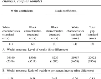
We now turn to wealth accumulation, which we measure using the five-year changes between the 1984 and 1989 surveys or between the 1989 and 1994 surveys. These show a much more rapid rate of accumulation for whites than for blacks. In the trimmed sample, for example, the mean five-year change in wealth including home equity is 36,160 for whites and 8,237 for blacks. The corresponding values for W/yare 1.28 and 0.45, respectively. The large difference could reflect dif-ferences in savings, difdif-ferences in rates of return on assets, or a combination of the two.
How much of the difference in accumulation rates can be explained by differences in income and demographics? To answer this question, we estimate growth models that include the variables that appear in the wealth models plus the changes in the measures of current income, region, SMSA, wife’s work hours, children, dependents, health status, and self-employment. To ensure reasonable sample sizes we confine the analysis to couples. We do not weight observations in computing the decompositions. The wealth change decompositions are reported in Table 4. In the case of W, income and demographic variables explain 74 percent of the difference in accumulation rates when the accumulation model for whites is used. Using the accumulation model for blacks, the same factors explain 49 percent of the gap. The corresponding figures for The Journal of Human Resources
growth in the wealth/permanent income ratio, W/y, is 84 percent based on the white accumulation model and 30 percent based on the black accumulation model. In sum-mary, we find that income and demographic characteristics explained more of the gap in wealth accumulation when the wealth model for whites is used.
What is responsible for the substantial difference between blacks and whites in the sensitivity of wealth levels and wealth/permanent income ratios to income and demo-graphic variables? Difference in the rate of return to wealth may be part of the story, because blacks have larger percentages of their wealth in home equity and smaller percentages in stocks and business wealth. However, the differences seem too great to be attributable to differences in rate of return alone although further research on this issue is needed. The wealth change regressions suggest that differences in savings rates are an important factor. Recall that our sibling results show that inheritances and gifts are not a major factor in the black/white differences in the wealth models. This fact, in combination with the substantial race differences in the wealth growth mod-els, suggests that differences in savings behavior, possibly in combination with rates
Altonji and Doraszelki 25
Table 4
Mean regression decompositions of the race gap in growth of wealth (5 year changes, couples sample)
White coefficients Black coefficients
Explained Explained gap using gap using
white black
White Black Black White Total coefficients coefficients
characteristics characteristics characteristics characteristics gap (standard (standard
(standard (standard (standard (standard (standard error) error)
error) error) error) error) error) (percent) (percent)
(1) (2) (3) (4) (5) (6) (7)
A. Wealth measure: Level of wealth (first difference)
36160 15366 8237 21967 27922 20794 13730
(2306) (5511) (1685) (4668) (2856) (5006) (4353)
(74%) (49%)
B. Wealth measure: Ratio of wealth to permanent income (first difference)
1.28 0.58 0.45 0.70 0.83 0.70 0.25
(0.05) (0.12) (0.06) (0.17) (0.08) (0.11) (0.16)
(84%) (30%)
C. Wealth measure: Log of wealth (first difference)
0.39 0.37 0.15 0.33 0.23 0.01 0.18
(0.02) (0.06) (0.06) (0.14) (0.06) (0.05) (0.13)
(5%) (77%)
of return, may be an important source of the wealth gap and of black/white differences in the wealth models.14
Note that the results for logs in Panel C of Table 4 present a challenge to the above interpretation. The results for logs show that 77 percent of the wealth is explained when the black log wealth growth model is used while only 5 percent of the gap is explained when the white log wealth growth model is used. These results are not con-sistent with the results in Panels A and B and cannot be attributed to the fact that the log model is basically a multiplicative specification. We do not have a good explana-tion for this, but note that many of the coefficients in the model are poorly estimated and the explanatory power of both the white model and black model is low. In general, the low explanatory power of the growth models makes us cautious in interpreting the decompositions, especially in the case of the models for blacks.15
In independent work, Gittleman and Wolff (2001) analyze race differences in wealth accumulation using a different approach than ours. They find that race differ-ences in savings rates are entirely explained by differdiffer-ences in income and demo-graphics. Because they pool whites and blacks and use population weights, their regression estimates should be close to those for the white sample. Thus, their results for savings are qualitatively consistent with our results for the change in W/y, although we only explain 84 percent of the gap in the change in W/y.
VII. Conclusions and Further Questions
Using better income and demographic controls than were available for previous studies, we can explain a large part of the racial disparity in wealth hold-ings with income and demographic variables provided that we estimate the wealth model on a sample of whites, but only a small fraction when we use the black wealth model. We also find that a higher self-employment rate and a stronger link between self-employment and wealth for whites than for blacks make an important contribution to the wealth gap between white and black couples. Overall, our results suggest that race differences in the sensitivity of wealth to income and demographics may be as important as the gap in income and demographics in understanding black/white differences in wealth.
What underlies the substantial race differences in the sensitivity of wealth holding to income and demographics? The fact that we obtain similar results when we relate sibling differences in wealth to sibling differences in income and demographics sug-gests, perhaps surprisingly, that differences in inter vivos transfers and inheritances are not the main reason the wealth model coefficients differ by race. This would seem to leave race differences in savings behavior and/or rates of return as a default The Journal of Human Resources
26
14. We have also estimated equations for W that include a lagged value of W along with the other variables used in the savings regressions. However, given the presence of lagged wealth, the high explanatory power of the models is largely due to the race gap in lagged wealth, and so it is hard to know what the economic significance of the explained gap is. See Footnote 29 of AD for details.
15. The adjusted R2s of the growth models are only about 0.05 for the growth in ln W. The adjusted R2is
explanation. We find that income and demographic differences explain a substantial part of the difference between whites and blacks in the growth in the level of wealth and in the ratio of wealth to permanent income when we use the wealth model for whites, but relatively little when we use the wealth model for blacks. This result points to important differences between whites and blacks in the effects of income and demographics on savings and/or rates of return, although this conclusion is tentative for a number of reasons discussed above. We suspect that differences in savings behavior is the main factor. This conjecture is supported by the fact that about 25–30 percent of black households are “unbanked,” meaning that they have no direct access to a financial institution (Hogarth and O’Donnell 1999; Hogarth and Lee 2000).
A large research agenda remains. Our sibling approach to the study of the effects of parental resources on the wealth models should be augmented by a study of the sources of intergenerational links in wealth along the lines of recent work by Charles and Hurst (2002). The role of self-employment and small business forma-tion has already received a substantial amount of attenforma-tion in the literature and deserves more.
As suggested by Smith (1995), a possible explanation for the racial disparity in sav-ings behavior is that differences in permanent income in conjunction with lower life expectancies among blacks and a higher replacement rate of private income with pub-licly provided social security and health benefits depress the incentive to save for retirement of blacks relative to whites.16 Lower life expectancy for blacks should
reduce savings, although we doubt that it plays a major role.
The lower incomes of black households may lead to greater dependence on social transfer programs relative to own resources and private transfers, holding permanent income and other household characteristics constant. Eligibility requirements for many transfer programs, including welfare programs and public housing, discourage wealth accumulation. This may reduce the private incentive to accumulate wealth.17
Another possible explanation revolves around the implications of differences in the income distributions of the friends and relatives of whites versus blacks. The basic idea is that savings and wealth accumulation are influenced by economic links to other households and friends that are motivated by altruism or other factors. The effects of ties to other households on savings depends on the level and distribution of resources and needs. We know that wealth is a convex function of permanent income. An explanation for this is that the marginal utility of household consumption declines in spending, leading households to accumulate resources as a hedge against future consumption needs, fluctuations in income, and uncertainty about the lifespan. Unspent resources are left to children or to charity late in life or upon death. However, if a high-income family has strong ties to needy relatives and friends, it may make transfers rather than accumulate wealth. Also, social pressure on the relatively
well-Altonji and Doraszelki 27
16. In preliminary work using the Health and Retirement Survey (HRS), John Karl Scholz (University of Wisconsin–Madison) has found that the race gap is much smaller for pensions than other forms of wealth (personal communication). This could have spillovers into holding of assets.