Ileana Ioan. 185KB Jun 04 2011 12:09:02 AM

(1)

ON THE OPTOELECTRONIC IMPLEMENTATION OF

NEURAL NETWORKS. SOURCES OF ERRORS AND

THEIR INFLUENCE ON THE INFLUENCE OF RANDOM

DEVIATIONS OF THE WEIGHTS ON THE

PERFORMANCES

Ioan Ilean , Joldeş Remus

Abstract.

One of the most promising implementation of neural networks is optoelectronic implementation. Optical interconnections are useful for neural networks as far as one can take advantage of the special potential of 3D connection through free space. This paper analyses the consequences caused by random deviations of the neurons interconnection weights from the accurately computed values. For the neural network we used, the connections are considered to be implemented optically, by computer generated holograms (CGH) and we outlined the main causes of weight deviations. Also we study the influence of these deviations on the network’s dynamics, accuracy of prototype recall, spurious states etc. The theoretical results are sustained by simulations of a concrete autoassociative neural network.

Keywords: Autoassociative memory, weights matrix, random deviations, pattern

recognition.

1.INTRODUCTION

The artificial neural networks have the specific feature of “storing” the knowledge in the synaptic weights of the processing elements (artificial neurons).There is a great number of algorithms allowing the design of neural networks (e. g.2) and the computing of weight values.

(2)

It is expected that these deviations of the weights from the accurate values influence the network’s behaviour during the working phase. This paper therefore intends an analysis of the consequences of synaptic weights deviations from the accurate values in the particular case of an associative network, whose neurons are optically interconnected through CGH.

Section 2 briefly presents the network model we used, as well as some results concerning the behaviour of this network type. Section 3 reviews the main causes of errors that may occur when using CGH to implement the interconnections of neurons. Section 4 realises a detailed study on the consequences of the random weights deviations on the behaviour of the network and section 5 shows the results of some simulations realised by the authors.

2. THE ARTIFICIAL NEURAL NETWORK MODEL

In this section we’ll briefly introduce the main theoretical elements concerning associative memories and recurrent neural networks 4, elements that will be used in section 5 in order to build an associative memory for patterns recognition.

We’ll call pattern a multidimensional vector with real components. An associative memory is a system that accomplishes the association of p pattern pairs

n

R ∈

µ

ξ , ςµ∈Rn, (µ=1, 2,..., p) so that when the system is given a new vector n

R

x∈ such as

)

(

min

)

(

j

j i

d

x

,

ξ

=

x

,

ξ

(1)

the system responds with ςi; in (1) d(a,b) is the distance between patterns a and b.

The pairs

( )

ξi,ςi , (i= 1,2,... p) are called prototypes and the association accomplished by the memory can be defined as a transformation Φ: Rn ×Rm so that

( )

i

i ξ

ς =Φ .

The space Ω⊂Rn of input vectors x is named configuration space and the vectors ξi, (i=1,2,...,p) are called attractors or stable points. Around each attractor, there is a basin of attraction Bi such that ∀x∈Bi, the dynamics of the network will

lead to the stabilization of

( )

ξi,ςi pair. For autoassociative memories ξi =ςi

(i=1,2,...,p) and if some vector x is nearest ξi, then Φ

( )

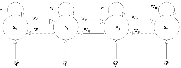
x =ξi.

In section 4 we will use for graphic pattern recognition a neural network whose model4 is presented below. Let’s consider the single-layer neural network built from totally connected neurons, whose states are given by xi∈{-1,1}, i=1,2,... n, (fig.1).

We denote : W=[wij,: 1≤ i, j≤ n] the weights matrix, θ=[θ1, ..., θn]T∈Rn the

(3)

For the memory described in this paper, the weight matrix W will be built as follows: given a set of n-dimensional prototype vectors X=[ξ1, ξ 2,..., ξp ], we establish the synaptic matrix W and the threshold vector θ, so that the prototype vectors become stable points for the associative memory, that is:

ξ

i

=

sgn(

W

ξ

i

−

θ

)

i

=

1,

2,..,

p

(2) where the sgn function is applied to each component of the argument.

w11 wii wjj wnn

wnj

wjn

wji

wij

wi1

w1i

x

1

x

i

x

j

x

n [image:3.595.115.489.196.337.2]

!1k !ik !jk !nk

Fig. 1. Single layer recurrent neural network

We use the Lyapunov method to study the stability of the network, defining an energy function and showing that this function is decreasing for any network trajectory in the state space. In our case, we’ll consider the following energy function:

x

T

Wx

-

x

T

θ

2

1

)

(

=

−

E

(3)

where x is the network state vector at time t.

From the evolution in states space point of view, a network can reach a stable point or can execute a limit cycle. At its turn, a stable point can be a global or a local energy minimum. Using (3), the following results concerning the network’s dynamics are demonstrated in4:

a) The asynchronous updating mode:

Χ If the synaptic matrix is symmetric and has non-negative diagonal elements, the recurrent network in asynchronous operation has only stable states (there are no cycles). As a consequence, the different variants of Hebb’s law (weighted, with or without null diagonal) and the projection rule guarantee the absence of cycles for asynchronous mode.

b) The synchronous updating mode:

(4)

cycles in synchronous mode. If the diagonal is null, two-length cycles may appear.

3. ERROR SOURCES FOR OPTICAL INTERCONNECTION WITH CGH

Optical interconnections are useful for neural networks as far as one can take advantage of the special potential of 3D connection through free space. This involves the organizing of the neurons layer in 2D configurations (planar), where the optical interconnections realise the desired links between the two planes. A certain connection also materialises the synaptic weight corresponding to neuron j from input plane and neuron i from output plane (fig. 2).

The interconnection network accomplishes the following function:

∑

⋅

=

ij

ijkl

T

j

i

l

k

,

)

(

,

)

(

α

β

(4)

In order to connect the two neuron planes one may use computer generated holograms which, by light waves diffraction, assure the desired connections. Due to the fact that generally the connections differ from neuron to neuron, the interconnection system will be a spatial variant system, each point from the input plane being connected differently to the output plane. This spatial variance can be realised in several manners.

(i,j)

Input plane

(Photonic generators or SLM)

Optical interconnectionnetwork Output plane (Photodetectors)

(k,l)

Fig. 2 .Optical interconnection of two neural planes.

Implementing optical interconnection with CGH implies the following steps:

• synthesis 8 of CGH for the synaptic weights matrix W (fig. 3)

CGH Complex

amplitude calculation

[image:4.595.107.489.361.473.2]

Coding Materialization

(5)

In the following we will briefly review the errors that may occur in the optical implementation of interconnections, leading to deviations of the real weight values from the accurate ones.

A. During the CGH computing step, the errors are due to the hologram synthesis method, as well as to the quantization of the obtained values 7, 8,10,11. When using Fourier amplitude holograms, a frequent difficulty is connected to the dynamic range of Fourier coefficients to be materialized in hologram. The computed range would lead to a smaller number of large aperture cells, most of the apertures being small, which significantly diminishes the hologram efficience on diffraction. Consequently, a dynamic range compression is required, with direct influence on the accuracy of the resulting synaptic weights.

During the CGH materialization step, the errors may occur from the unsatisfactory resolution of the devices involved or from the photolythographic process.

B. During the building of optical setup (the hardware implementation of the neural network), the following error sources may appear:

• Un-uniform optical emission of the photoemitters from the output plane of the neural layer (the input plane of the optical interconnection system)

• Un-uniform sensitivity of the photodetectors in the input plane of the neural layer (the output plane of the optical interconnection system)

• Axial misalignment (translation or rotation) of the three planes: the input plane, the hologram plane and the output plane.

• Errors concerning the positioning of individual photoemitters or photodetectors in their corresponding plane.

• Errors due to the variation of the geometrical dimensions of the setup, as a result of temperature variations.

• Errors caused by interaction of the adjacent optical paths (the light flow deviated by the hologram to a certain photodetector also reaches the nearby photodetectors).

All the errors above can be minimized, but it is obvious they cannot be completely removed. Consequently, we find very useful an analysis of the influences these errors might have on the global behaviour of the network.

4. INFLUENCE OF RANDOM WEIGHT DEVIATIONS

In the following, we will present a general qualitative study on the effects of the weight deviations from the accurate values. We’ll denote by W the accurate (theoretical) weight matrix and by W *the real weight matrix. We may then consider:

W W

W*= +

δ

(5)

where ∗W is a matrix of deviations from the computed values.

(6)

network. In order to simplify the computing we will consider null thresholds for all the neurons. The network’s dynamics is associated to this energy function and one can easily see that the weight values deviations will have important consequences on the network’s functioning.

Thus, the random deviations of synaptic weights values can cancel the symmetry of W matrix and the property of diagonal elements (e. g. they may become negative), making the results in section 2 (concerning stability) no longer valid. A non-symmetric or negative diagonal weight matrix may lead to the occurrence of cycles in the network’s evolution. Therefore, the network won’t reach a stable state, consequently it won’t work well as associative memory.

The weight matrix synthesis starts from a set of prototype vectors we wish to be stored. From energy perspective, these prototypes are global minimum of function E (of value E0). If instead of the accurate W matrix the network operates using the W

*

matrix, the energy value for some prototype becomes:

E

ξ

=

ξ

−

ξ

δ

ξ

=

₀

+

δ

2

1

2

1

(

)

-

T

W

T

W

(6)

One may observe that the weights deviation from accurate values will modify the “energy landscape”. The prototypes minimum may change, as well as spurious states minimums may occur.

Up to this point we didn’t make any assumption on the range or statistical distribution of deviations. Now we will perform, following3, a more detailed analysis, to see the influence of deviations on the maximum number of prototypes the memory can store. For this, starting from the dynamic equation with θi= 0, we’ll study the

stability of component ξiυ(i=1,2,..,n) of the prototype ξυ:

∑

₌ =

∑

₌ +

∑

₌ = n j n j n j j ij j ij j ij

i w w w

1 1 1

*

) sgn(

)

sgn( ν ν

ν

ξ

δ

ξ

(7)

We’ll call net input (or synaptic potential):

∑

₌ =

∑

₌ +

∑

₌ = n j n j n j j ij j ij j ij

i w w w

h

1 1 1

* ν ν

ν

ξ

δ

ξ

₍₈₎

Assuming that the weights have been computed using Hebb’s rule, it is easy to outline the contribution of ξ_iυ to net input:

∑∑

₌ _≠ +

∑

₌ + = n j n j j ij j j i i i w n h 1 1 1 ν µ ν ν µ µ ν

ν

ξ

δ

ξ

₍₉₎

where µ:=1,2,..,p indexes the p prototypes.

We denote by Zi the additive term from (14) and we make the observation that if

(7)

prototypes that may be stored, we’ll consider: ) 1 ( 1 1

∑∑

₌ _≠ +

∑

₌ − = ⋅ − = n j n j j ij j j i i i i i w n Z C ν µ ν ν µ µ ν ν

ν

ξ

δ

ξ

₍₁₀₎

The probability for ξ_iυ to be unstable is (remember that ξ_imay take only -1 or +1 values):

)

1

(

Pr

>

=

ν i unst

ob

C

p

(11)

We shall try to find the distribution function and the statistical parameters for the random variable Cυi .

Let

∑∑

₌ _≠ − = n j j j i i i n A 1 1 ν µ ν µ µ ν

ξ

(12)

and

∑

₌ − = n j j ij i i w B 1 ν ν

δ

ξ

(13)

In the reference [3] it is shown that the variable Ai obeys, with a good

approximation, a gaussian distribution with mean 0 and variance p/n. We’ll consider that the deviations δ Wij also obey a gaussian distribution with mean 0 and variance

2 δ

σ . In this case, the variable Bi will obey, with a good approximation, a gaussian

distribution with mean 0 and variance σ_δ2. Consequently, we may assume that variable Ci obeys a normal distribution with mean 0 and variance:

2 2 δ

σ

=

+

n

p

(14) We denote 2

'

=

p

+

n

⋅

σ

_δ

p

(15)

and using the results from reference [3] we find that the correct functioning of the network implies

138

.

0

'

≤

n

p

(16) or

n

p

≤

(

0

.

138

−

σ

_δ2

)

⋅

(17) One can thus see that random deviations of the weights can seriously affect

(8)

5. EXPERIMENTAL RESULTS AND CONCLUSIONS

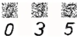
We’ve performed a large number of simulations in order to verify the theoretical considerations from the precedent section. We’ve studied an autoassociative neural network, synthesized starting from a set of 10 prototypes representing the cursive script numerals 0..9 (fig. 4). The simulations have had in view the influence that random weight deviations have on the following network features:

• Noise tolerance. The network had to recognize noise affected prototypes, using the accurate W matrix, and also the deviated weights matrix W *.

• The energy minimums corresponding to prototypes. For the 10 prototypes we have computed the energy minimums, in the accurate weights phase, as well as using the deviated weights.

• The average number of iterations before stabilizing into an attractor.

Fig.4. The prototypes used in simulations

The results we’ve obtained are illustrated below:

[image:8.595.238.368.376.443.2]

I. When the associative memory operates with the accurate weights, it shows a very good noise immunity, recognizing prototypes affected by up to 40% noise (fig. 5).

Fig. 5. The recognition of noisy prototypes by the accurate network

If the weight matrix used is W*, the noise immunity decreases, so that the network is no longer able to recognize prototypes with the same noise contamination (fig.6).

In order to study the above mentioned objectives, we’ve performed several simulations affecting the weight matrix W with random deviations having various distribution laws and parameters.

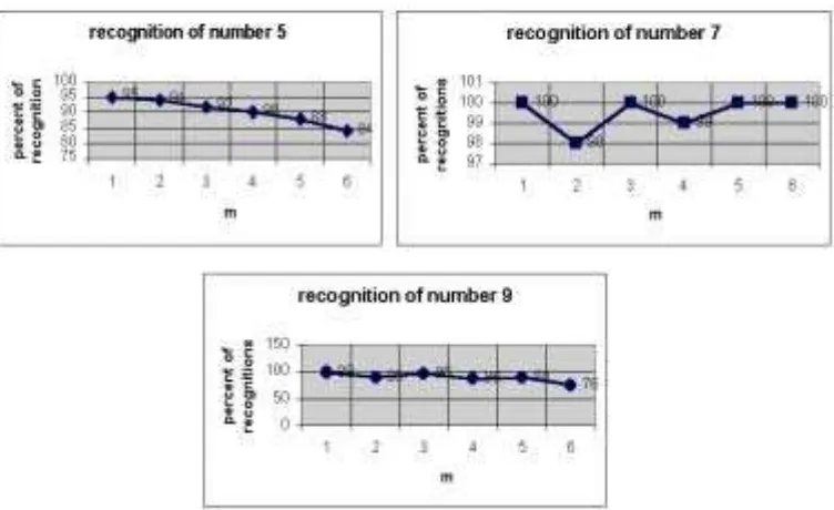
A first set of simulations pursued the altering of the accurate matrix with random deviations having a gaussian distribution, with different mean and variance values. For each case, we’ve performed 100 recognitions of every prototype, disturbed by 40% noise. The results are shown in fig. 7.

(9)

its value. In this case also we’ve performed 100 recognitions for each noise affected prototype. The results are shown in table 1.

[image:9.595.253.355.203.305.2]

II. For every deviated matrix we used, we’ve computed the prototype corresponding energy values, watching the energy minimum’s variations. The simulations outlined, for the above cases, a slight disturbance of the energy minimums (about 3% of the values corresponding to the accurate weights). Also, we’ve noticed that the average number of iterations slightly varies from the value of 3, no matter which the weights deviations are.

Fig. 6. Failed recognition of prototypes by the deviated weights network

Fig. 7. Recognition of some noisy prototypes by the network with weights disturbed by Gaussian deviations with variance Φ_∗2−m2Φw2

[image:9.595.119.495.339.569.2]

(10)

Prototype 0 1 2 3 4 5 6 7 8 9

Percent of correct recognitions

94 100 94 81 95 86 98 100 98 91

CONCLUSIONS

The simulations have shown diminished performances of the autoassociative memory as a result of the random weights deviations from the correctly computed values. For the statistical parameters used above the performances’ degradation is relatively small, which proves certain insensitivity to those deviations. Therefore, the memory appears quite robust, not only in what the noise contained by the patterns to be recognized is concerned, but also in relation with the random weights deviations.

It is possible for this insensitivity to occur also due to the fact that the number of stored prototypes is much lower than the memory’s capacity. The simulations performed on another associative memory, designed to recognize cursive script letters, confirm this last assumption. In this case the input vector’s size is still of 1024 components, but the amount of stored prototypes becomes 27.

This aspect is to be elucidated in further studies. It would also be useful to determine quantitatively the contribution of the errors described in section 4 to the deviation of actual weights from accurate ones, in order to state realistic requests for the hardware implementation of the autoassociative memory.

REFERENCES

1. Cox J. A., Werner T., Lee J., Nelson S., Fritz B. and Bergshom J.: “Diffraction efficiency of binary optical elements. Proc. SPIE vol. 1211, pp.116-124 (1990). 2. Dumitra∏ Adriana: Proiectarea re⇔elelor neuronale artificiale, Casa editorial|

Odeon, Bucure∏ti, 1997.

3. Hertz John, Krogh Anders, Palmer G. Richard: Introduction to the theory of

neural computation, Addison-Wesley Publishing Company, 1991.

4. Kamp Yves, Hasler Martin:Reseaux de neurones récursifs pour mémoires associatives,Presses polytechniques et universitairea romandes, Lausanne, 1990. 5. Keller E. Paul and Gmitro F. Arthur: “ Computer-generated holograms for optical

neural networks: on-axis versus off-axis geometry”, Applied Optics 32, pp.1304-1310 (10 March 1993).

6. Keller E. Paul and Gmitro F. Arthur: “Design and analysis of fixed planar holographic interconnects for optical neural networks”. Applied Optics 31, pp.5517-5526, 10 September 1992.

7. Lee Hon Wai: “Sampled Fourier Transform Hologram Generated by Computer”,

(11)

8. Lohmann A. W. and Paris D. P.: “Binary Fraunhofer Holograms, Generated by Computer, Applied Optics, Vol 6 (10), pp.1739-1745 (October 1967).

9. Riehl J., Appel J. Thiriot A., Dorey J.: “Hybrid electronic/non coherent optical processor for large scale phased arrays”. SPIE vol. 963 Optical Computing 88, pp.337-345.

10. Seldowitz A. Michael, Allebach Jan P., and Sweeney W. Donald: “Synthesis of digital holograms by direct binary search”, Applied Optics,vol 26, No. 14/ 15 July 1987, pp.2788-2798.

11. Wolf E.: Progress in Optics XXVIII, Elsevier Science Publishers B. V. 1990.