El e c t ro n ic
Jo ur
n a l o
f P
r o
b a b il i t y
Vol. 14 (2009), Paper no. 70, pages 2038–2067. Journal URL
http://www.math.washington.edu/~ejpecp/
Depinning of a polymer in a multi-interface medium
∗
F. Caravenna
Dipartimento di Matematica Pura e Applicata
Università degli Studi di Padova,
via Trieste 63
35121 Padova
Italy
Email: [email protected]
N. Pétrélis
Institute of Mathematics
University of Zürich
Winterthurerstrasse 190
8057 Zürich
Switzerland
Email: [email protected]
Abstract
In this paper we consider a model which describes a polymer chain interacting with an infinity of equi-spaced linear interfaces. The distance between two consecutive interfaces is denoted by
T = TN and is allowed to grow with the size N of the polymer. When the polymer receives a positive reward for touching the interfaces, its asymptotic behavior has been derived in[3], showing that a transition occurs whenTN ≈logN. In the present paper, we deal with the so– calleddepinning case, i.e., the polymer is repelled rather than attracted by the interfaces. Using techniques from renewal theory, we determine the scaling behavior of the model for largeNas a function of{TN}N, showing that two transitions occur, whenTN ≈N1/3and whenTN ≈pN
respectively.
Key words: Polymer Model, Pinning Model, Random Walk, Renewal Theory, Localiza-tion/Delocalization Transition.
AMS 2000 Subject Classification:Primary 60K35, 60F05, 82B41.
Submitted to EJP on January 17, 2009, final version accepted July 21, 2009.
∗We gratefully acknowledge the support of the Swiss Scientific Foundation (N.P. under grant 200020-116348) and of
1
Introduction and main results
1.1
The model
We consider a(1+1)-dimensional model of a polymer depinned at an infinity of equi-spaced hori-zontal interfaces. The possible configurations of the polymer are modeled by the trajectories of the simple random walk(i,Si)i≥0, whereS0 = 0 and(Si−Si−1)i≥1 is an i.i.d. sequence of symmetric Bernouilli trials taking values 1 and−1, that is P(Si−Si−1 = +1) = P(Si−Si−1 = −1) = 12. The
polymer receives an energetic penaltyδ <0 each times it touches one of the horizontal interfaces lo-cated at heights{kT:k∈Z}, whereT∈2N(we assume thatT is even for notational convenience). More precisely, the polymer interacts with the interfaces through the following Hamiltonian:
HNT,δ(S) := δ
N
X
i=1
1{Si∈TZ} = δ X
k∈Z
N
X
i=1
1{Si=k T}, (1.1)
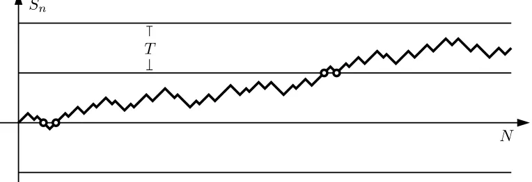
where N ∈N is the number of monomers constituting the polymer. We then introduce the corre-sponding polymer measurePNT,δ(see Figure 1 for a graphical description) by
dPNT,δ dP (S) :=
exp HNT,δ(S)
ZNT,δ , (1.2)
where the normalizing constantZNT,δ=E[exp(HNT,δ(S))]is called thepartition function.
S
n [image:2.612.71.453.414.545.2]N
T
Figure 1: A typical path of{Sn}0≤n≤N under the polymer measure PTN,δ, for N =158 and T =16. The circles indicate the points where the polymer touches the interfaces, that are penalized byδ <0 each.
We are interested in the case where the interface spacing T ={TN}N≥1 is allowed to vary with the
For the reader’s convenience, and in order to get some intuition on our model, we recall briefly the result obtained in[3]forδ >0. We first set some notation: given a positive sequence {aN}N, we write SN ≍ aN to indicate that, on the one hand, SN/aN is tight (for everyǫ > 0 there exists M > 0 such that PTN
N,δ |SN/aN| > M
≤ ǫ for large N) and, on the other hand, that for some
ρ∈(0, 1)andη >0 we havePTN
N,δ |SN/aN|> η
≥ρfor largeN. This notation catches the rate of asymptotic growth ofSN somehow precisely: ifSN≍aN andSN ≍bN, for someǫ >0 we must have
ǫaN ≤bN ≤ǫ−1aN, for largeN.
Theorem 2 in[3]can be read as follows: for everyδ >0 there existscδ>0 such that
SN underPTN
N,δ ≍
p N e−
cδ
2TNT
N if TN− c1
δ logN→ −∞ TN if TN− c1
δ logN=O(1) 1 if TN− c1
δ logN→+∞
. (1.3)
Let us give an heuristic explanation for these scalings. For fixedT∈2N, the process{Sn}0≤n≤N under PNT,δbehaves approximately like a time-homogeneous Markov process (for a precise statement in this direction see §2.2). A quantity of basic interest is the first timeτˆ:=inf{n>0 : |Sn|=T}at which the polymer visits a neighboring interface. It turns out that forδ >0 the typical size ofτˆis of order ≈ecδT, so that until epochN the polymer will make approximatelyN/ecδT changes of interface. Assuming that these arguments can be applied also when T = TN varies with N, it follows that the process {Sn}0≤n≤N jumps from an interface to a neighboring one a number of times which is approximately uN := N/ecδTN. By symmetry, the probability of jumping to the neighboring upper
interface is the same as the probability of jumping to the lower one, hence the last visited interface will be approximately the square root of the number of jumps. Therefore, when uN → ∞, one expects thatSN will be typically of order TN ·puN, which matches perfectly with the first line of (1.3). On the other hand, whenuN →0 the polymer will never visit any interface different from the one located at zero and, because of the attractive reward δ >0, SN will be typically at finite distance from this interface, in agreement with the third line of (1.3). Finally, whenuN is bounded, the polymer visits a finite number of different interfaces and thereforeSN will be of the same order asTN, as the second line of (1.3) shows.
1.2
The main results
Also in the repulsive caseδ <0 one can perform an analogous heuristic analysis. The big difference with respect to the attractive case is the following: under PTN,δ, the time τˆ the polymer needs to jump from an interface to a neighboring one turns out to be typically of orderT3 (see Section 2). Assuming that these considerations can be applied also to the case when T = TN varies with N, we conclude that, underPTN
N,δ, the total number of jumps from an interface to the neighboring one should be of order vN :=N/TN3. One can therefore conjecture that if vN →+∞the typical size of SN should be of orderTN·pvN=pN/TN, while if vN remains bounded one should haveSN≍TN.
should be of orderTN, while ifTN≫pN we should haveSN ≍pN (of course we writeaN ≪bN iff aN/bN →0 and aN ≫bN iff aN/bN →+∞). We can sum up these considerations in the following formula:
SN ≍
p
N/TN if TN ≪N1/3
TN if (const.)N1/3≤TN≤(const.)pN p
N if TN ≫pN
. (1.4)
It turns out that these conjectures are indeed correct: the following theorem makes this precise, together with some details on the scaling laws.
Theorem 1.1. Letδ <0and{TN}N∈N∈(2N) N
be such that TN→ ∞as N→ ∞.
(1) If TN ≪N1/3, then SN ≍
p
N/TN. More precisely, there exist two constants0< c1 < c2 <∞
such that for all a,b∈Rwith a<b we have for N large enough
c1Pa<Z≤b ≤ PTN
N,δ
a<
SN
Cδ
q
N TN
≤ b
≤ c2P
a<Z≤b, (1.5)
where Cδ:=π/
p
e−δ−1is an explicit positive constant and Z∼ N(0, 1).
(2) If TN ∼ (const.)N1/3, then SN ≍ TN. More precisely, for every ǫ >0small enough there exist constants M,η >0such that∀N ∈N
PTN
N,δ |SN| ≤M TN
≥ 1−ǫ, PTN
N,δ |SN| ≥ηTN
≥ 1−ǫ. (1.6)
(3) If N1/3≪TN ≤(const.) p
N , then SN ≍TN. More precisely, for everyǫ >0small enough there exist constants L,η >0such that∀N∈N
PTN
N,δ 0<|Sn|<TN, ∀n∈ {L, . . . ,N}
≥ 1−ǫ, PTN
N,δ |SN| ≥ηTN
≥ 1−ǫ. (1.7)
(4) If TN ≫ p
N , then SN ≍ p
N . More precisely, for everyǫ >0small enough there exist constants L,M,η >0such that∀N ∈N
PTN
N,δ 0<|Sn|<M p
N, ∀n∈ {L, . . . ,N} ≥ 1−ǫ, PTN
N,δ |SN| ≥η p
N ≥ 1−ǫ. (1.8)
To have a more intuitive view on the scaling behaviors in (1.4), let us consider the concrete example TN ∼(const.)Na: in this case we have
SN ≍
N(1−a)/2 if 0≤a≤ 13 Na if 13 ≤a≤ 12 N1/2 ifa≥ 12
. (1.9)
We have thus shown that the asymptotic behavior of our model displays two transitions, atTN≈pN and at TN ≈ N1/3. While the first one is somewhat natural, in view of the diffusive behavior of the simple random walk, the transition happening at TN ≈ N1/3 is certainly more surprising and somehow unexpected.
Let us make some further comments on Theorem 1.1.
• About regime (1), that is whenTN≪N1/3, we conjecture that equation (1.5) can be strength-ened to a full convergence in distribution:SN/(Cδ
p
N/TN) =⇒ N(0, 1). The reason for the slightly weaker result that we present is that we miss sharp renewal theory estimates for a basic renewal process, that we define in §2.2. As a matter of fact, using the techniques in
[7]one can refine our proof and show that the full convergence in distribution holds true in the restricted regime TN ≪ N1/6, but we omit the details for conciseness (see however the discussion following Proposition 2.3).
In any case, equation (1.5) implies that the sequence {SN/(Cδ
p
N/TN)}N is tight, and the limit law of any converging subsequence must be absolutely continuous with respect to the Lebesgue measure on R, with density bounded from above and from below by a multiple of the standard normal density.
• The case when TN →T ∈Ras N→ ∞has not been included in Theorem 1.1 for the sake of simplicity. However a straightforward adaptation of our proof shows that in this case equation (1.5) still holds true, withCδreplaced by a different (T-dependent) constantCbδ(T).
• We stress that in regimes (3) and (4) the polymer really touches the interface at zero a finite number of times, after which it does not touch any other interface.
1.3
A link with a polymer in a slit
It turns out that our modelPTN,δis closely related to a model which has received quite some attention in the recent physical literature, the so-calledpolymer confined between two walls and interacting with them[1; 6; 8](also known as polymer in a slit). The model can be simply described as follows: givenN,T∈2N, take the firstNsteps of the simple random walk constrained not to exit the interval {0,T}, and give each trajectory a reward/penalizationγ∈Reach time it touches 0 orT (one can also consider two different rewards/penaltiesγ0 andγT, but we will stick to the caseγ0=γT =γ). We are thus considering the probability measureQTN,γdefined by
dQTN,γ
dPNc,T (S) ∝ exp γ N
X
i=1
1{S
i=0 orSi=T}
!
, (1.10)
where PNc,T(·) := P(· |0 ≤ Si ≤ T for all 0 ≤ i ≤ N) is the law of the simple random walk con-strainedto stay between the two walls located at 0 andT.
Consider now the simple random walkreflected on both walls 0 and T, which may be defined as {ΦT(Sn)}n≥0, where({Sn}n≥0,P)is the ordinary simple random walk and
ΦT(x) := min[x]2T, 2T−[x]2T , with [x]2T := 2T
x
2T −
j x
2T
k
0 0 T
T 2T 3T
−T δ
δ δ δ δ
δ+ log 2 δ+ log 2
[image:6.612.79.452.87.282.2]ΦT
Figure 2: A polymer trajectory in a multi-interface medium transformed, after reflection on the interfaces 0 and T, in a trajectory of polymer in a slit. The dotted lines correspond to the parts of trajectory that appear upside-down after the reflection.
that is,[x]2T denotes the equivalence class of x modulo 2T (see Figure 2 for a graphical descrip-tion). We denote byPNr,T the law of the firstNsteps of{ΦT(Sn)}n≥0. Of course,PNr,T is different from PNc,T: the latter is the uniform measure on the simple random walk paths {Sn}0≤n≤N that stay in {0,T}, while under the former each such path has a probability which is proportional to 2NN, where NN=PNi=11{Si=0 orSi=T}is the number of times the path has touched the walls. In other terms, we
have
dPNc,T
dPNr,T(S) ∝ exp −(log 2) N
X
i=1
1{Si=0 orSi=T}
!
. (1.11)
If we consider the reflection underΦT of our model, that is the process{ΦT(Sn)}0≤n≤N underPNT,δ, whose law will be simply denoted byΦT(PTN,δ), then it comes
dΦT(PTN,δ)
dPNr,T (S) ∝ exp δ N
X
i=1
1{S
i=0 orSi=T}
!
. (1.12)
At this stage, a look at equations (1.10), (1.11) and (1.12) points out the link with our model: we have the basic identity QTN,δ+log 2 = ΦT(PTN,δ), for all δ ∈ R and T,N ∈ 2N. In words, the polymer confined between two attractive walls is just the reflection of our model throughΦT, up to a shift of the pinning intensity by log 2. This allows a direct translation of all our results in this new framework.
Let us describe in detail a particular issue, namely, the study of the modelQTN,γ whenT =TN is al-lowed to vary withN(this is interesting, e.g., in order to interpolate between the two extreme cases when one of the two quantitiesT andNtends to∞before the other). This problem is considered in
Focusing on the casea= b=exp(γ), we mention in particular equations (6.4)–(6.6) in[8], which fora<2 read as
Zn,w(a,a) ≈ (const.) n3/2 fphase
p n w
, (1.13)
where we have neglected a combinatorial factor 2n (which just comes from a different choice of notation), and where the function fphase(x)is such that
fphase(x) → 1 as x→0 , fphase(x) ≈ x3e−π
2x2/2
as x → ∞. (1.14)
The regime a < 2 corresponds to γ < log 2, hence, in view of the correspondence δ = γ−log 2 described above, we are exactly in the regime δ < 0 for our model PNT,δ. We recall (1.2) and, with the help of equation (2.11), we can express the partition function with boundary condition SN∈(2T)Zas
ZNT,,δ{SN∈(2T)Z} ∼ O(1)ZT,{SN∈TZ}
N,δ ∼ O(1)e φ(δ,T)N
Pδ,T(N∈τ),
where, with some abuse of notation, we denote byO(1)a quantity which stays bounded away from 0 and∞asN → ∞. In this formula,φ(δ,T)is thefree energyof our model and({τn}n∈Z+,Pδ,T) is a basic renewal process, introduced respectively in §2.1 and §2.2 below. In the case when T = TN → ∞, we can use the asymptotic expansion (2.3) forφ(δ,T), which, combined with the bounds in (2.21), gives asN,T→ ∞
ZT,{SN∈(2T)Z}
N,δ =
O(1)
N3/2 max
1,
pN
T
3
exp
−π
2
2 N T2 +
2π2
e−δ−1 N T3 +o
N
T3
.
SinceZT,{SN∈(2T)Z}
N,δ =Zn,w(a,a), we can rewrite this relation using the notation of[8]:
Zn,w(a,a) ≈ (const.) n3/2 fphase
p
n w
g
n1/3
w
, where g(x) ≈ e 2π2
e−δ−1x as x→ ∞.
We have therefore obtained a refinement of equations (1.13), (1.14). This is linked to the fact that we have gone beyond the first order in the asymptotic expansion of the free energyφ(δ,T), making an additional term of the orderN/TN3 appear. We stress that this new term gives a non-negligible (in fact, exponentially diverging!) contribution as soon asTN≪N1/3(w≪n1/3 in the notation of[8]). This corresponds to the fact that, by Theorem 1.1, the trajectories that touch the walls a number of times of the orderN/TN3 are actually dominating the partition function whenTN ≪N1/3. Of course, a higher order expansion of the free energy (cf. Appendix A.1) may lead to further correction terms.
1.4
Outline of the paper
the renewal function, which are of crucial importance for the proof of Theorem 1.1. Sections 3, 4, 5 and 6 are dedicated respectively to the proof of parts (1), (2), (3) and (4) of Theorem 1.1. Finally, some technical results are proven in the appendices.
We stress that the value ofδ <0 is kept fixed throughout the paper, so that the generic constants appearing in the proofs may beδ-dependent.
2
A renewal theory viewpoint
In this section we recall some features of our model, including a basic renewal theory representation, originally proven in[3], and we derive some new estimates.
2.1
The free energy
Considering for a moment our model whenTN ≡ T ∈2Nis fixed, i.e., it does not vary with N, we define thefree energy φ(δ,T) as the rate of exponential growth of the partition function ZNT,δ as N→ ∞:
φ(δ,T) := lim N→∞
1 N logZ
T
N,δ = Nlim→∞ 1 N logE
eHTN,δ
. (2.1)
Generally speaking, the reason for looking at this function is that the values ofδ(if any) at which
δ 7→ φ(δ,T) is not analytic correspond physically to the occurrence of aphase transition in the system. As a matter of fact, in our case δ7→ φ(δ,T) is analytic on the whole real line, for every T ∈2N. Nevertheless, the free energy φ(δ,T) turns out to be a very useful tool to obtain a path description of our model, even when T = TN varies with N, as we explain in detail in §2.2. For this reason, we now recall some basic facts onφ(δ,T), that were proven in[3], and we derive its asymptotic behavior asT→ ∞.
We introduce τT1 := inf{n > 0 : Sn ∈ {−T, 0,+T}}, that is the first epoch at which the polymer visits an interface, and we denote byQT(λ):=E e−λτ
T
1its Laplace transform under the law of the simple random walk. We point out thatQT(λ) is finite and analytic on the interval(λT0,∞), where
λ0T <0, andQT(λ)→+∞asλ↓λT0 (as a matter of fact, one can give a closed explicit expression forQT(λ), cf. equations (A.4) and (A.5) in [3]). A basic fact is that QT(·) is sharply linked to the free energy: more precisely, we have
φ(δ,T) = (QT)−1(e−δ), (2.2)
for everyδ∈R(see Theorem 1 in[3]). From this, it is easy to obtain an asymptotic expansion of
φ(δ,T)asT → ∞, forδ <0, which reads as
φ(δ,T) = − π
2
2T2
1− 4 e−δ−1
1 T +o
1
T
, (2.3)
2.2
A renewal theory interpretation
We now recall a basic renewal theory description of our model, that was proven in §2.2 of[3]. We have already introduced the first epochτT
1 at which the polymer visits an interface. Let us extend
this definition: forT∈2N∪ {∞}, we setτ0T =0 and for j∈N
τTj := infn> τTj−1: Sn∈TZ and ǫT j :=
SτT j−
SτT j−1
T , (2.4)
where for T=∞we agree thatTZ={0}. Plainly,τT
j is the j
thepoch at whichS visits an interface
andǫTj tells whether the jth visited interface is the same as the(j−1)th (ǫTj =0), or the one above (ǫTj =1) or below (ǫTj =−1). We denote byqTj(n)the joint law of (τ1T,ǫ1T)under the law of the simple random walk:
qTj(n) := P τT1 =n,ǫ1T = j. (2.5) Of course, by symmetry we have thatq1T(n) =qT−1(n)for everynandT. We also set
qT(n) := P τ1T =n
= q0T(n) +2q1T(n). (2.6)
Next we introduce a Markov chain({(τj,ǫj)}j≥0,Pδ,T)taking values in(N∪{0})×{−1, 0, 1}, defined in the following way:τ0 :=ǫ0 :=0 and underPδ,T the sequence of vectors {(τj−τj−1,ǫj)}j≥1 is
i.i.d. with marginal distribution
Pδ,T(τ1=n,ǫ1= j) := eδq
j T(n)e−
φ(δ,T)n. (2.7)
The fact that the r.h.s. of this equation indeed defines a probability law follows from (2.2), which implies thatQ(φ(δ,T)) =E(e−φ(δ,T)τ1T) =e−δ. Notice that the process{τ
j}j≥0alone underPδ,T is a (undelayed)renewal process, i.e.τ0=0 and the variables{τj−τj−1}j≥1are i.i.d., with step law
Pδ,T(τ1=n) = eδqT(n)e−φ(δ,T)n = eδP(τT1 =n)e−
φ(δ,T)n. (2.8)
Let us now make the link between the lawPδ,T and our modelPTN,δ. We introduce two variables that count how many epochs have taken place beforeN, in the processesτT andτrespectively:
LN,T := supn≥0 : τTn ≤N , LN := supn≥0 : τn≤N . (2.9)
We then have the following crucial result (cf. equation (2.13) in[3]): for allN,T ∈2Nand for all k∈N,{ti}1≤i≤k∈Nk,{σi}1≤i≤k∈ {−1, 0,+1}kwe have
PTN,δLN,T =k, (τiT,ǫiT) = (ti,σi), 1≤i≤k
N∈τT
= Pδ,TLN =k, (τi,ǫi) = (ti,σi), 1≤i≤k
N∈τ,
(2.10)
where{N∈τ}:=S∞k=0{τk=N}and analogously for{N ∈τT}. In words, the process{(τTj,ǫ T j)}j under PTN,δ(· |N ∈τT) is distributed like the Markov chain {(τj,ǫj)}j under Pδ,T(· |N ∈ τ). It is precisely this link with renewal theory that makes our model amenable to precise estimates. Note that the lawPδ,T carries no explicit dependence on N. Another basic relation we are going to use repeatedly is the following one:
EheHkT,δ(S)1
{k∈τT}
i
= eφ(δ,T)kPδ,T k∈τ, (2.11)
2.3
Some asymptotic estimates
We now derive some estimates that will be used throughout the paper. We start from the asymptotic behavior ofP(τT
1 =n)asn→ ∞. Let us set
g(T) := −log cos
π
T
= π
2
2T2 +O
1
T4
, (T→ ∞). (2.12)
We then have the following
Lemma 2.1. There exist positive constants T0,c1,c2,c3,c4 such that when T > T0 the following rela-tions hold for every n∈2N:
c1
min{T3,n3/2}e
−g(T)n
≤ P(τ1T =n) ≤ c2
min{T3,n3/2}e
−g(T)n, (2.13)
c3 min{T,pn}e
−g(T)n
≤ P(τ1T >n) ≤ c4 min{T,pn}e
−g(T)n. (2.14)
The proof of Lemma 2.1 is somewhat technical and is deferred to Appendix B.1. Next we turn to the study of the renewal process {τn}n≥0,Pδ,T
. It turns out that the law ofτ1underPδ,T is essentially split into two components: the first one atO(1), with masseδ, and the second one atO(T3), with mass 1−eδ (although we do not fully prove these results, it is useful to keep them in mind). We start with the following estimates onPδ,T(τ1=n), which follow quite easily from Lemma 2.1.
Lemma 2.2. There exist positive constants T0,c1,c2,c3,c4 such that when T > T0 the following rela-tions hold for every m,n∈2N∪ {+∞}with m<n:
c1
min{T3,k3/2}e
−(g(T)+φ(δ,T))k
≤ Pδ,T(τ1=k) ≤
c2
min{T3,k3/2}e
−(g(T)+φ(δ,T))k (2.15)
Pδ,T(m≤τ1<n) ≥ c3
e−(g(T)+φ(δ,T))m−e−(g(T)+φ(δ,T))n (2.16) Pδ,T(τ1≥m) ≤ c4e−(g(T)+φ(δ,T))m. (2.17)
Proof. Equation (2.15) is an immediate consequence of equations (2.8) and (2.13). To prove (2.16), we sum the lower bound in (2.15) overk, estimating min{T3,k3/2} ≤T3and observing that by (2.3) and (2.12), for every fixedδ <0, we have asT → ∞
g(T) +φ(δ,T) = 2π
2
e−δ−1 1
T3 1+o(1)
. (2.18)
To get (2.17), form≤T2there is nothing to prove (provided c4is large enough, see (2.18)), while
form>T2 it suffices to sum the upper bound in (2.15) overk.
Notice that equation (2.15), together with (2.18), shows indeed that the law ofτ1has a component
are the following ones:
Eδ,T(τ1) =
eδ(e−δ−1)2 2π2 T
3 + o(T3), (2.19)
Eδ,T(τ21) =
eδ(e−δ−1)3 2π4 T
6 + o(T6), (2.20)
which are proven in Appendix A.2. We stress that these relations, together with equation (A.6), imply that, underPδ,T, the timeτˆneeded to hop from an interface to a neighboring one is of order T3, and this is precisely the reason why the asymptotic behavior of our model has a transition at TN ≈ N1/3, as discussed in the introduction. Finally, we state an estimate on the renewal function Pδ,T(n∈τ), which is proven in Appendix B.2.
Proposition 2.3. There exist positive constants T0,c1,c2 such that for T > T0 and for all n∈2Nwe have
c1
min{n3/2,T3} ≤ Pδ,T(n∈τ) ≤
c2
min{n3/2,T3}. (2.21)
Note that the large nbehavior of (2.21) is consistent with the classical renewal theorem, because 1/Eδ,T(τ1)≈ T−3, by (2.19). One could hope to refine this estimate, e.g., proving that forn≫T3
one hasPδ,T(n∈τ) = (1+o(1))/Eδ,T(τ1): this would allow strengthening part (1) of Theorem 1.1
to a full convergence in distributionSN/(Cδ
p
N/TN) =⇒ N(0, 1). It is actually possible to do this forn≫T6, using the ideas and techniques of[7], thus strengthening Theorem 1.1 in the restricted regimeTN ≪N1/6 (we omit the details).
3
Proof of Theorem 1.1: part (1)
We are in the regime whenN/TN3→ ∞asN→ ∞. The scheme of this proof is actually very similar to the one of the proof of part (i) of Theorem 2 in [3]. However, more technical difficulties arise in this context, essentially because, in the depinning case (δ <0), the density of contact between the polymer and the interfaces vanishes asN→ ∞, whereas it is strictly positive in the pinning case (δ >0). For this reason, it is necessary to display this proof in detail.
Throughout the proof we set vδ = (1−eδ)/2 and kN =⌊N/Eδ,TN(τ1)⌋. Recalling (2.4) and (2.9),
we setYTN
0 =0 andY
TN
i =ǫ TN
1 +· · ·+ǫ
TN
i fori∈ {1, . . . ,LN,TN}. Plainly, we can write
SN = YTN
LN,TN ·TN + sN, with |sN| < TN. (3.1)
In view of equation (2.19), this relation shows that to prove (1.5) we can equivalently replace SN/(Cδ
p
N/TN)withYTN
LN,TN/
p
3.1
Step 1
Recall (2.7) and setYn=ǫ1+· · ·+ǫnfor alln≥1. The first step consists in proving that for alla<b inR
lim N→∞ Pδ,TN
a< YkN
p
vδkN ≤ b
= P(a<Z≤ b), (3.2)
that is, underPδ,T
N and asN→ ∞we haveYkN/
p
vδkN =⇒Z, where “=⇒” denotes convergence in distribution.
The random variables(ǫ1, . . . ,ǫN), defined under Pδ,TN, are symmetric and i.i.d. . Moreover, they
take their values in{−1, 0, 1}, which together with (A.6) entails
Eδ,TN(|ǫ1|
3) =
Eδ,TN((ǫ1)
2)
−→ vδ asN→ ∞. (3.3)
Observe thatkN → ∞asN → ∞andEδ,T
N(τ1) =O(T
3
N), by (2.19). Thus, we can apply the Berry Esseèn Theorem that directly proves (3.2) and completes this step.
3.2
Step 2
Henceforth, we fix a sequence of integers(VN)N≥1 such that TN3 ≪VN ≪N. In this step we prove that, for alla<b∈R, the following convergence occurs, uniformly inu∈ {0, . . . , 2VN}:
lim N→∞ Pδ,TN
a< pYLN−u
vδkN ≤ b
= P(a<Z≤b). (3.4)
To obtain (3.4), it is sufficient to prove that, asN→ ∞and under the lawPδ,T
N,
UN:= YkN
p
vδkN
=⇒Z and GN := sup
u∈{0,...,2VN}
YL
N−u−YkN
p
vδkN
=⇒0 . (3.5)
Step 1 gives directly the first relation in (3.5). To deal with the second relation, we must show that Pδ,TN(GN ≥ ǫ)→ 0 asN → ∞, for allǫ >0. To this purpose, notice that {GN ≥ ǫ} ⊆A
N η∪B
N η,ǫ, where forη >0 we have set
ANη:=LN−kN≥ηkN ∪LN−2V
N−kN ≤ −ηkN (3.6)
BηN,ǫ:=
¨
supYkN+i−YkN
p
vδkN
, i∈ {−ηkN, . . . ,ηkN}
≥ǫ
«
. (3.7)
Let us focus onPδ,T
N(A
N
η). Introducing the centered variablesτfk:=τk−k· Eδ,TN(τ1), fork∈N, by
the Chebychev inequality we can write (assuming that(1−η)kN∈Nfor notational convenience)
Pδ,TN LN−2VN−kN<−ηkN
= Pδ,T
N τ(1−η)kN >N−2VN
= Pδ,T
N τe(1−η)kN >N−2VN−(1−η)kNEδ,TN(τ1) = ηN−2VN
≤ (1−η)kNVarδ,TN(τ1)
(ηN−2VN)2
≤ N Varδ,TN(τ1)
(ηN−2VN)2Eδ,TN(τ1)
With the help of the estimates in (2.19), (2.20), we can assert that Varδ,T
N(τ1)/Eδ,TN(τ1) =O(T
3
N). Since N ≫ VN andN ≫ TN3, the r.h.s. of (3.8) vanishes asN → ∞. With a similar technique, we prove thatPδ,TN LN−kN > ηkN
→0 as well, and consequentlyPδ,TN(A
N
η)→0 asN→ ∞.
At this stage it remains to show that, for every fixedǫ > 0, the quantity Pδ,TN B
N η,ǫ
vanishes as
η→0,uniformly inN. This holds true because{Yn}nunderPδ,TN is a symmetric random walk, and therefore{(Yk
N+j−YkN)
2
}j≥0 is a submartingale (and the same with j 7→ −j). Thus, the maximal
inequality yields
Pδ,TN B
N η,ǫ
≤ 2
ǫ
Eδ,TN (YkN+ηkN−YkN)
2
vδkN ≤
2ηEδ,TN(ǫ
2 1)
ǫvδ ≤
2η ǫvδ
. (3.9)
We can therefore assert that the r.h.s in (3.9) tends to 0 asη→0, uniformly inN. This completes the step.
3.3
Step 3
Recall thatkN =⌊N/Eδ,TN(τ1)⌋. In this step we assume for simplicity thatN ∈2N, and we aim at
switching from the free measurePδ,TN toPδ,TN · N ∈τ. More precisely, we want to prove that there exist two constants 0<c1<c2<∞such that for alla< b∈Rthere exists N0>0 such that
forN≥N0 and for allu∈ {0, . . . ,VN} ∩2N
c1P(a<Z≤b) ≤ Pδ,T
N
a< YLN−u
p
vδkN ≤ b
N−u∈τ
≤ c2P(a<Z≤b). (3.10)
A first observation is that we can safely replace LN−u with LN−u−T3
N in (3.10). To prove this, since
kN→ ∞, the following bound is sufficient: for everyN,M∈2N
sup u∈{0,...,VN}∩2N
Pδ,TN
YLN
−u−YLN−u−T3
N
≥M
N−u∈τ
≤ (const.)
M . (3.11)
Note that the l.h.s. is bounded above byPδ,TN #
τ∩[N−u−TN3,N−u) ≥ MN−u∈τ. By time-inversion and the renewal property we then rewrite this as
Pδ,TN #
τ∩(0,TN3] ≥MN−u∈τ = Pδ,T
N τM ≤T
3
N
N−u∈τ
≤ TN3
X
n=1
Pδ,TN τM=n
·Pδ,TN N−u−n∈τ
Pδ,TN N−u∈τ
.
(3.12)
Recalling that N ≫VN ≫ TN3 and using the estimate (2.21), we see that the ratio in the r.h.s. of (3.12) is bounded above by some constant, uniformly for 0≤n≤TN3 andu∈ {0, . . . ,VN} ∩2N. We are therefore left with estimatingPδ,T
N τM≤T
3
N
. Recalling the definitionτek:=τk−k·Eδ,T(τ1)∼
τk−ckT3 asT→ ∞, wherec>0 by (2.19), it follows that for largeN∈Nwe have
Pδ,TN(τ∩[0,T
3
N]≥M) = Pδ,TN(τM ≤T
3
N)
≤ Pδ,TN
e
τM≤ − c 2M T
3
N
≤ 4M Varδ,TN(τ1)
c2M2TN6 ≤
having applied the Chebychev inequality and (2.20). This proves (3.11).
Let us come back to (3.10). By summing over the last point inτbefore N−u−TN3 (call itN−u− TN3−t) and the first point inτafterN−u−TN3 (call itN−u−TN3+r), using the Markov property we obtain
Pδ,TN
a<
YLN −u−T3
N
p
vδkN ≤b
N−u∈τ
= N−T3
N−u
X
t=0
Pδ,TN
a<
YL
N−u−TN3−t
p
vδkN
≤b,N−u−TN3−t∈τ
· Pδ,TN τ1>t
·Θuδ,N(t),
(3.13)
whereΘuδ,N is defined by
Θuδ,N(t) :=
PT3
N
r=1Pδ,TN τ1=t+r
· Pδ,TN T
3
N−r∈τ
Pδ,TN N−u∈τ
· Pδ,TN τ1>t
. (3.14)
Let us setINu:={0, . . . ,N−u−TN3}. Notice that replacingΘuδ,N(t)by the constant 1 in the r.h.s. of (3.13), the latter becomes equal to
Pδ,TN
a<
YLN −u−T3
N
p
vδkN ≤b
. (3.15)
Sinceu+TN3 ≤2VN for large N (becauseVN ≫TN3), equation (3.4) implies that (3.15) converges asN → ∞toP(a<Z≤ b), uniformly foru∈ {0, . . . ,VN} ∩2N. Therefore, equation (3.10) will be proven (completing this step) once we show that there existsN0such thatΘuδ,N(t)is bounded from above and below by two constants 0 < l1 < l2 < ∞, forN ≥ N0 and for all u∈ {0, . . . ,VN}and t∈ INu.
Let us set KN(n) := Pδ,TN(τ1 = n) and uN(n) := Pδ,TN(n∈ τ). The lower bound is obtained by
restricting the sum in the numerator of (3.14) to r ∈ {1, . . . ,TN3/2}. Recalling that N ≫VN ≫TN3, and applying the upper (resp. lower) bound in (2.21) touN(N−u)(resp.uN(TN3−r)), we have that for largeN, uniformly inu∈ {0, . . . ,VN}andt∈ INu,
Θuδ,N(t) ≥
PT3
N/2
r=1 KN(t+r)·uN TN3−r
uN N−u
·P∞j=1KN(t+j)
≥ c1 c2·
PT3
N/2
r=1 KN(t+r)
P∞
j=1KN(t+j)
. (3.16)
Then, we use (2.16) to bound from below the numerator in the r.h.s. of (3.16) and we use (2.17) to bound from above its denominator. This allows to write
Θuδ,N(t) ≥ c1c3(1−e
−(g(TN)+φ(δ,TN)) T3
N
2 )
c2c4 . (3.17)
The upper bound is obtained by splitting the r.h.s. of (3.14) into
RN+DN :=
PT3
N/2
r=1 KN(t+r)·uN(TN3−r) uN N−u
·P∞j=1KN(t+ j) +
PT3
N/2
r=1 KN(t+TN3−r)·uN(r) uN N−u
·P∞j=1KN(t+ j)
. (3.18)
The termRN can be bounded from above by a constant by simply applying the upper bound in (2.21) touN(TN3−r)for allr∈ {1, . . . ,T
3
N/2}and the lower bound touN(N−u). To boundDN from above, we use the upper bound in (2.15), which, together with the fact that g(TN) +φ(δ,TN)∼mδ/TN3, shows that there existsc>0 such that forN large enough andr∈ {1, . . . ,TN3/2}we have
KN(t+TN3−r)≤ c
TN3 e
−(g(TN)+φ(δ,TN))t. (3.19)
Notice also that by (2.16) we can assert that
∞
X
j=1
KN(t+j)≥c3e−(g(TN)+φ(δ,TN))t. (3.20)
Finally, (3.19), (3.20) and the fact thatuN(N−u)≥c1/TN3 for allu∈ {0, . . . ,VN}(by (2.21)) allow to write
DN ≤ c
PT3
N/2
r=1 uN(r) c1c3
. (3.21)
By applying the upper bound in (2.21), we can check easily thatPT 3
N/2
r=1 uN(r)is bounded from above uniformly inN≥1 by a constant. This completes the proof of the step.
3.4
Step 4
In this step we complete the proof of Theorem 1.1 (1), by proving equation (1.5), that we rewrite for convenience: there exist 0<c1 <c2<∞such that for alla< b∈Rand for largeN ∈2N(for
simplicity)
c1P(a<Z≤b) ≤ PTN
N,δ
a<
YTN
LN
p
vδkN ≤b
≤ c2P(a<Z≤ b). (3.22)
We recall (2.4) and we start summing over the locationµN:=τ TN
LN,TN of the last point inτ
TN before
N:
PTN
N,δ
a<
YTN
LN,TN
p
vδkN ≤ b
= N
X
ℓ=0
PTN
N,δ
a<
YTN
LN,TN
p
vδkN ≤ b
µN=N−ℓ
·PTN
N,δ µN =N−ℓ
. (3.23)
Of course, only the terms withℓeven are non-zero. We want to show that the sum in the r.h.s. of (3.23) can be restricted toℓ ∈ {0, . . . ,VN}. To that aim, we need to prove thatPNℓ=V
NP
TN
N,δ µN = N−ℓtends to 0 asN→ ∞. We start by displaying a lower bound on the partition function ZTN
Lemma 3.1. There exists a constant c>0such that for N large enough
ZTN
N,δ ≥ c TN e
φ(δ,TN)N. (3.24)
Proof. Summing over the location ofµN and using the Markov property, together with (2.11), we have
ZTN
N,δ = E
h
eHNTN,δ(S)
i = N X r=0 E h
eHNTN,δ(S)1
{µN=r}
i
= N
X
r=0
EheHrTN,δ(S)1
{r∈τTN}
i
P(τTN
1 >N−r)
= N
X
r=0
eφ(δ,TN)rPδ
,TN(r∈τ)P(τ
TN
1 >N−r). (3.25)
From (3.25) and the lower bounds in (2.14) and (2.21), we obtain forN large enough
ZTN
N,δ ≥ (const.)e
φ(δ,TN)N
N
X
r=0
e−[φ(δ,TN)+g(TN)](N−r)
min{pN−r+1,TN}min{(r+1)3/2,T3
N}
. (3.26)
At this stage, we recall thatφ(δ,T) +g(T) =mδ/T3+o(1/T3)asT→ ∞, withmδ>0, by (2.18). SinceTN3 ≪N, we can restrict the sum in (3.26) to r∈ {N−TN3, . . . ,N−TN2}, for largeN, obtaining
ZTN
N,δ ≥ (const.)
eφ(δ,TN)N
TN4
N−T2
N
X
r=N−T3
N
e−
mδ TN3+o
1
TN3
(N−r)
≥ (const.′)e
φ(δ,TN)N
TN , (3.27)
because the geometric sum gives a contribution of orderTN3.
We can now bound from above (using the Markov property and (2.11))
NX−VN
l=0
PTN
N,δ(µN=ℓ) = NX−VN
ℓ=0
E exp HTN
ℓ,δ(S)
1{ℓ∈τ}·P τ1>N−ℓ
ZTN
N,δ
= NX−VN
ℓ=0
Pδ,TN(ℓ∈τ)e
φ(δ,TN)ℓ P τ
1>N−ℓ
ZTN
N,δ
≤ (const.) NX−VN
ℓ=0
TN
min{(ℓ+1)3/2,T3
N} ·e
−[φ(δ,TN)+g(TN)](N−ℓ)
min{pN−ℓ,TN}
, (3.28)
where we have used Lemma 3.1 and the upper bounds in (2.14) and (2.21). For notational conve-nience we setd(TN) =φ(δ,TN)+g(TN). Then, the estimate (2.18) and the fact thatVN ≫TN3 imply that
NX−VN
ℓ=0
PTN
n,δ(µN =ℓ) ≤ (const.)e−d(TN)VN NX−VN
ℓ=0
e−d(TN)(N−VN−ℓ)
min{(ℓ+1)3/2,T3
N}
≤ (const.′)e−d(TN)VN
X∞
ℓ=0
1
(l+1)3/2 +
∞
X
ℓ=0
e−d(TN)(ℓ)
TN3
.
Sinced(TN)∼ mδ/TN3, withmδ>0, andVN ≫TN3 we obtain that the l.h.s. of (3.29) tends to 0 as N→ ∞.
Thus, we can write
PTN
N,δ
a<
YTN
LN,TN
p
vδkN ≤b
= VN
X
ℓ=0
PTN
N,δ
a<
YTN
LN,TN
p
vδkN ≤b
µN =N−ℓ
PTN
N,δ µN=N−ℓ
+ ǫN(a,b),
(3.30)
where ǫN(a,b)tends to 0 as N → ∞, uniformly overa,b∈R. At this stage, by using the Markov property and (2.10) we may write
PTN
N,δ
a<
YTN
LN,TN
p
vδkN ≤b
µN=N−ℓ
= PTN
N,δ
a<
YTN
LN−ℓ,TN
p
vδkN ≤b
N−ℓ∈τ
T
= Pδ,T
N
a< YLN−ℓ
p
vδkN ≤ b
N−ℓ∈τ
.
Plugging this into (3.30), recalling (3.10) and the fact thatPVN
ℓ=0P
TN
N,δ(µN =N−ℓ)→1 (by (3.29)), it follows that equation (3.22) is proven, and the proof is complete.
4
Proof of Theorem 1.1: part (2)
We assume thatTN ∼(const.)N1/3 and we start proving the first relation in (1.6), that we rewrite as follows: for everyǫ >0 we can find M>0 such that for largeN
PTN
N,δ |SN|>M·TN
≤ǫ.
Recalling that LTN is the number of times the polymer has touched an interface up to epoch N, see (2.9), we have|SN| ≤TN·(LN,TN +1), hence it suffices to show that
PTN
N,δ LN,TN >M
≤ǫ. (4.1)
By using (2.10) we have
PTN
N,δ LN,T >M
= 1
ZTN
N,δ E
h
eHNTN,δ(S)1
{LN,TN>M}
i
= 1
ZTN
N,δ N
X
r=0
EheHrTN,δ(S)1
{Lr,TN>M}1{r∈τTN}
i
P(τTN
1 >N−r)
= 1
ZTN
N,δ N
X
r=0
eφ(δ,TN)rPδ
,TN Lr,TN >M, r∈τ
TNP(τTN
By (2.14) and (2.12) it follows easily that
ZTN
N,δ ≥ P(τ TN
1 >N) ≥
(const.) TN e
−2π2
TN2N (4.2)
(note that this bound holds true whenever we have(const.)N1/4≤TN ≤(const.′) p
N for largeN). Using this lower bound onZTN
N,δ, together with the upper bound in (2.14), the asymptotic expansions in (2.18) and (2.12), we obtain
PTN
N,δ LN,T >M
≤ (const.)TN N
X
r=0
Pδ,TN Lr,TN >M,r∈τ
TN 1
min{pN−r+1,TN} .
The contribution of the terms withr>N−TN2 is bounded with the upper bound (2.21):
TN N
X
r=N−T2
N
1
TN3
1 p
N−r+1 ≤
(const.)
TN −→ 0 (N→ ∞),
while for the terms with r≤N−TN2 we get
TN N
X
r=0
Pδ,TN Lr,TN >M,r ∈τ
TN 1
TN = Eδ,TN (LN,TN−M)1{LN,TN>M}
.
Finally, we simply observe that{LN,T
N =k} ⊆
Tk
i=1{τi−τi−1≤N}, hence
Pδ,TN(LN,TN =k) ≤ Pδ,TN(τ1≤N)
k ≤ ck,
with 0<c<1, as it follows from (2.16) and (2.18) recalling thatN=O(TN3). Putting together the preceding estimates, we have
PTN
N,δ LN,TN >M
≤ (const.)Eδ,T
N (LN,TN−M)1{LN,TN>M}
= (const.)
∞
X
k=M+1
(k−M)Pδ,T
N(LN,TN =k)
≤ (const.)
∞
X
k=M+1
(k−M)ck ≤ (const.′)cM,
and (4.1) is proven by choosingM sufficiently large.
Finally, we prove at the same time the second relations in (1.6) and (1.7), by showing that for every
ǫ >0 there existsη >0 such that for largeN
PTN
N,δ |SN| ≤ηTN
≤ ǫ, (4.3)
invariance principle that there existsc>0 such that inf0≤k≤ηT
NPk(τ ∞
1 ≤η 2T2
N, Si<TN∀i≤τ∞1 )≥
c for largeN. Therefore we may write
cPTN
N,δ |SN| ≤ηTN
= c
ZTN
N,δ ηTN
X
k=0
EheHNTN,δ(S)1
{|SN|=k}
i
≤ 1
ZTN
N,δ ηTN
X
k=0
η2T2
N
X
u=0
E
h
eHNTN,δ(S)1
{|SN|=k}
i
Pk(τ∞1 =u, Si<TN∀i≤u)
= 1
ZTN
N,δ ηTN
X
k=0
η2T2
N
X
u=0
E
h
eHNTN+u,δ(S)1
{|SN|=k}1{|SN+i|<TN∀i≤u}1{SN+u=0}
i
.
Performing the sum over k, dropping the second indicator function and using equations (2.11), (2.21) and (2.3), we obtain the estimate
PTN
N,δ |SN| ≤ηTN
≤ 1
c ZTN
N,δ η2T2
N
X
u=0
E
h
eHNTN+u,δ(S)1
{N+u∈τTN}
i
≤ 1
c ZTN
N,δ η2T2
N
X
u=0
eφ(δ,TN)(N+u)Pδ
,TN(N+u∈τ) ≤ (const.) η2TN2 ZTN
N,δT
3
N e−
π2 2TN2N.
Then (4.2) shows that equation (4.3) holds true forηsmall, and we are done.
5
Proof of Theorem 1.1: part (3)
We now give the proof of part (3) of Theorem 1.1. More precisely, we prove the first relation in (1.7), because the second one has been proven at the end of Section 4 (see (4.3) and the following lines). We recall that we are in the regime whenN1/3≪TN≤(const.)pN, so that in particular
C := inf N∈N
N
TN2 > 0 . (5.1)
We start stating an immediate corollary of Proposition 2.3.
Corollary 5.1. For everyǫ >0there exist T0>0, Mǫ∈2N, dǫ>0such that for T >T0
dXǫT3
k=Mǫ
Pδ,T k∈τ
≤ ǫ.
Note that we can restate the first relation in (1.7) asPTN
N,δ τ TN
LN,TN ≤ L
≥1−ǫ. Let us define three intermediate quantities, by setting forl∈N
B1(l,N) = PTN
N,δ τ TN
LN,TN ≤l
ZTN
N,δ, (5.2)
B2(l,N) = P
TN
N,δ l< τ TN
LN,TN ≤N−ηT
2
N
ZTN
N,δ, (5.3)
B3(N) = PTN
N,δ τ TN
LN,TN >N−ηT
2
N
ZTN
where we fixη:=C/2, so thatηTN2 ≤N/2. The first relation in (1.7) will be proven once we show that for allǫ >0, there existslǫ∈Nsuch that for largeN we have
B2(lǫ,N)
B1(lǫ,N) ≤ ǫ and
B3(N)
B1(lǫ,N) ≤ ǫ. (5.5)
We start giving a simple lower bound ofB1: since{τ
TN
LN,TN ≤l} ⊇ {τ TN
1 >N}, we have
B1(l,N) ≥ E
h
eHNTN,δ(S)1
{τTN1 >N}
i
= P τTN
1 >N
≥ (const.) TN
e− π2
2TN2N,