ELECTRONIC
COMMUNICATIONS in PROBABILITY
FILTERING AND PARAMETER ESTIMATION FOR A
JUMP STOCHASTIC PROCESS WITH DISCRETE
OB-SERVATIONS
OLEG V MAKHNIN
Department of Mathematics, New Mexico Tech, Socorro NM 87801 email: [email protected]
Submitted October 31, 2006, accepted in final form February 18, 2008 AMS 2000 Subject classification: 60J75, 62M05, 93E11
Keywords: non-linear filtering, Kalman filter, particle filtering, jump processes, target tracking
Abstract
A compound Poisson process is considered. We estimate the current position of the stochas-tic process based on past discrete-time observations (non-linear discrete filtering problem) in Bayesian setting. We obtain bounds for the asymptotic rate of the expected square error of the filter when observations become frequent. The bounds depend linearly on jump intensity. Also, estimation of process’ parameters is addressed.
1
Introduction
Filtering of stochastic processes has attracted a lot of attention. One of the examples is target tracking, when a target is observed over a discrete time grid, corresponding to the successive passes of a radar. Another is signal processing, where the observations are discretized. In both cases, we deal with discrete observations.
We will further refer to the (unobservable) process of interest as “signal” (“state”)X(t). Assume that the time grid is uniform. We attempt to establish asymptotic properties of such filtering when the time interval τ between successive observations goes to zero. The signal+noise model takes the form of a state-space model: the processX(t) evaluated at the grid points is a discrete-time Markov process (see (1) below). The observation equation is
Yk=X(kτ) +ek, k= 1,2, ... where ek are i.i.d. with densityφ, mean 0 and varianceσ2
e.
The goal of filtering is to estimate the current position X(t) of the process based on all observations up to the moment. The filter given by
E[X(t)|Y1, ...Yk, τ k≤t < τ(k+ 1)]
is optimal with respect to square loss. That is, it minimizesE(X(t)−X(t))ˆ 2 among all filters ˆ
X(t) based on up-to-the-moment observations (see Lemma 1 below).
We consider a special case of stochastic process: piecewise-constant or pure-jump process. It is a compound Poisson process
X(t) =X0+ X i: si≤t
ξi
where (si, ξi) are the events of a 2-dimensional Poisson process on [0, T]×R. The intensity of this process is given byλ(s, y) =λh(y), whereλ >0 is a constant “time intensity” describing how frequently the jumps of X occur and h(y) = hθ(y) is the “jump density” describing magnitudes of jumpsξi of processX. Here θ ∈Θ⊂Rp is a parameter (possibly unknown) defining the distribution of jumps and errors.
In the Bayesian formulation, let parametersθandλhave a prior densityπ(θ, λ) with respect to Lebesgue measure. Assume that for eachθ∈Θ,Eξ2
1<∞. Also, assume that starting value X0 has some prior density π0(·). The Bayesian approach lends conveniently to the combined parameter and state estimation via the posterior expectation
\
(X(t), θ, λ) :=Eπ,π0[X(t), θ, λ |Y1, ...Yk, τ k≤t < τ(k+ 1)]
Remark 1
a) Generalizations to non-constant jump intensityλ=λ(·) and more general structure where λ(s, y) depends on current position ofX(s) are possible, but will not be considered here. b) A generalization to d-dimensional signal and observations is immediate when the density φof the error distribution takes a special form: φ(x1, ..., xd) =Qd
i=1φi(xi). In this case, the optimal filter can be computed coordinate-wise.
More realistic cases in context of target-tracking (like processes with pure-jump velocity or pure-jump acceleration) are more complex and will be discussed elsewhere. A special case of a piecewise-linear process with uniform observational errors was considered in [12], but their suggested asymptotics of O(n−2) appear to be incorrect. A general approach to filters for target-tracking was laid out in [11].
There is a substantial body of work dedicated to the filtering of jump processes in continuous noise (see [14] and references therein). In [13], jump processes of much more general type are considered, but the process is assumed to be observed without error.
Recently, considerable interest was devoted to practical methods of estimating the optimal filter. Particle filters described in [6] and [1] are useful, and have generated a great deal of interest in signal-processing community. Still, some convergence problems persist, especially when non-linearity of the model increases. Typically, the optimal filter is infinite-dimensional and requires great computational effort.
On the other hand, the popular Kalman filter (which is an optimallinearfilter, see, e.g., [4]) is fast but is based on the assumption of normality for both process and errors and may not be very efficient. In target-tracking literature, several low-cost improvements for Kalman filter have been suggested. In particular, interactive multiple model (IMM) filters were described in [2].
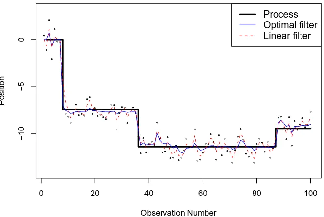
0 20 40 60 80 100
Figure 1: optimal non-linear and linear filters
and Kalman filters. Parameters areτ = 0.2,λ= 0.2, Normal jumps with mean 0 and variance = 52, and σe= 1.
One of the questions is how much improvement does the (optimal) non-linear filter bring compared to (linear) Kalman filter. Another is how does the error distribution affect this improvement.
2
Filtering of a jump process
2.1
Recursive formulation
DenotingXk:=X(τ k), we have
Xk=Xk−1+ζk (1)
Yk =Xk+ek
Here, ζk is a sum of jumps ofX on the interval [τ(k−1), τ k). Thus, {ζk}k≥1 are i.i.d. with an atom of mass e−λτ at 0 and the rest of the mass having (improper) density ˜ψ = ˜ψθ,λ expressible in terms of the original density of jumpshθ. To simplify the notation, I will callψ a “density”, actually meaning thatψ(0) is a scaledδ-function, that is for any functiong,
Z
g(x)ψ(x)dx:=e−λτ·g(0) +
Z
g(x) ˜ψ(x)dx Further on, subscriptsθ, λin φθ,ψθ,λ will be omitted.
The joint density ofX0:k:= (X0, ..., Xk),Y1:k:= (Y1, ..., Yk),θandλis found as p(x0:k, y1:k, θ, λ) =p(y1:k |x0:k, θ, λ)·p(x0:k |θ, λ)·π(θ, λ) = =π(θ, λ)·π0(x0)·
k
Y
j=1
φ(yj−xj)· k
Y
j=1
ψ(xj−xj−1) (2)
Let qk(x, θ, λ) := R
Rkp(x0:k, Y1:k, θ, λ)dx0... dxk−1 be the unnormalized density of the latest stateXk and parametersθ, λgiven the observationsY1:k. The following relation is well-known (see e.g. [6]).
Theorem 1.
q0(x, θ, λ) =πX0(x)·π(θ, λ),
qk(x, θ, λ) =φθ(Yk−x)·
Z
R
ψθ,λ(x−z)qk−1(z, θ, λ)dz= (3)
=φθ(Yk−x)·
e−λτqk−1(x, θ, λ) +
Z
R ˜
ψθ,λ(x−z)qk−1(z, θ, λ)dz
Remark 2
a) In order to use Theorem 1 for the estimation of stateXk, one should computeqj(x, θ, λ), j≤ kconsecutively, then compute marginal unnormalized densityqk(x) :=R
qk(x, θ, λ)dθ dλ and then find
ˆ
Xk:=E(Xk|Y1:k) =
R
Rxqk(x)dx R
Rqk(x)dx
. (4)
b) Although not derived explicitly, the unnormalized densityqhas to do with a change of the original probability measure to, say, Q, which makes the observationsY1, ..., Yk independent of the processX(t), see [7]. This way, prior distributions on (θ, λ) andX(0) ensure that the two measures are absolutely continuous with respect to each other. The change of measure approach is often used in non-linear filtering.
2.2
Multiple-block upper bound for expected square error
Next, we investigate asymptotic properties of the above filtering estimator ˆX(T) := ˆX⌊nT⌋ as
the observations become frequent (1/τ =n→ ∞). The following results were obtained when the error distribution is considered known. Without loss of generality, assumeT = 1 (since we can always rescale time, and use the new jump intensity λT). We assume that n is integer, so that the last jump occurs at exactly 1. If nis not integer, then the estimation of X(1) is based onY1, ..., Y⌊n⌋, and the expected loss added on the interval (τ⌊n⌋,1] is of order 1/n, so
the overall asymptotics will not change.
The following discussion is based on the well-known fact (e.g. see [3, p. 84])
Lemma 1. For a square-integrable random variableX, sigma-algebraF and anF-measurable random variable U,
E[X−E(X|F)]2≤E(X−U)2
Setting F := σ{Y1, ..., Yk}, we can see that the filtered estimator ˆXk introduced by (4) has the smallest expected square loss among all possible estimators of Xk based on observations Y1:k. We will produce a sub-optimal estimate forX(1) based on the mean of observations for a suitable interval. The difficulty lies in not knowing where exactly the last jump of process X occurred.
Consider the intervals (blocks) going backwards (T1, T0],(T2, T1], ...,(TN, TN−1], where
T0:= 1
Tj:=Tj−1−(lnn)j/n, j= 1, ..., N
and the total number of blocks is N :=⌊ln lnlnnn⌋ −1; j-th block has length (lnn)j/n and nj observations. The exact integer value ofnj depends on the positioning of blocks, but it differs from (lnn)j by no more than 1. Thus, in the future calculations we would sometimes use (lnn)j instead ofnj, as long as it will not change the asymptotic values of expressions. Note that the total length of all blocks, for nlarge enough, is no greater than
lnn n ·
(lnn)ln lnlnnn−1−1 lnn−1 =
n−lnn n(lnn−1) <1
Starting at the time 1, we will probe back one block of observations after another, stopping whenever we believe that a jump has occurred.
LetYj be the average of observations from the block j, that is Yj :=n−j1
X
k
YkI(Tj < k
n ≤Tj−1). Assumption 1. Let
χm:=
Pm
k=1ek
σe√m (5)
be the normalized sum of merrors. Assume that for the distribution of errorsek the following is true. There exist constants C1, C2 and K >0 such that for all sufficiently large m and uniformly for all positive integers j,
E[χ2mI(|χm|> C1·m
1
This assumption is satisfied for Normal errors with K= 2; in general, it requires ek to have small tails. The following is simpler-looking but more restrictive than Assumption 1:
Assumption 1′. For χm given above, there exist constants G, γ >0 such that for all
suffi-ciently largem,Eexp(γ|χm|)≤G.
Proposition 1. Assumption1′ implies Assumption 1 withK= 1.
Proof:
Suppose that Assumption 1′ is satisfied. Let Fm(.) be the distribution function ofχm. Pick
C1large enough, so thatx2<exp(γ
|x|/2) for|x|> C1, andγC1/2>1. Then for anyj,
Z
R
I{|x|> C1m1/j
}x2dFm(x)
≤
Z
R
I{|x|> C1m1/j
}eγ|x|/2dFm(x)
≤
≤exp(−γC1m1/j/2)Z R
eγ|x|dFm(x)
≤exp(−γC1m1/j/2)
·G
Theorem 2. Upper bound forE( ˆXn(1)−X(1))2
Suppose that the error density φ is known and does not depend on the parameter θ. Then, under Assumption 1, there exists a constant C such that for large enoughn,
E( ˆXn(1)−X(1))2
≤Cλln Mn
n withM =max{1 +K2,2}.
Proof:
ConsiderN blocks as described above. DenoteT⋆ the point of last jump ofX: T⋆= sup{0≤ t≤1 :X(t)−X(t−)>0}. Let alsoJ⋆= the number of Block where the last jump happened. The idea is to approximateT⋆, then take the average of all observations from that Block. Construct an estimate ofX(1) as follows. Definej0as
j0:=N∧
inf
j≥1 :√nj |Yj−Yj+1|
σe >2C1·n
1
Kj j
(6)
Then, as our estimate ofX(1), take ˜X(1) :=Yj0. We will find an upper bound for the average risk of this estimate,ℓ :=E( ˜X(1)−X(1))2. For this, we will need several inequalities, with proofs to follow in the next section.
Case 1: Correct stopping
In the event S that the last jump ofX occurred just before the Block j0, S={Tj0+1< T
⋆
≤Tj0}={J
⋆=j0+ 1
}
ℓS:=E[( ˜X(1)−X(1))2IS]≤C4λln 2n
n (7.1)
Case 2: Late stopping In the event L={Tj0 < T
⋆
}={J⋆
≤j0}
ℓL:=E[( ˜X(1)−X(1))2IL]≤C5λ(lnn)
(1+2/K)∨2
Case 3: Early stopping
rate of the estimator ˜X does not depend on the particular form of jump densityhθ.
By Lemma 1, the risk of estimate ˆX does not exceed the risk of ˜X. Even though the rate in (7.3) does not depend onλ, it is of a smaller order. Combining (7.1) through (7.3), we obtain the proof of the Theorem.
2.3
Proofs of inequalities used in Theorem 2
Proof of (7.1) randomness ofj0 and therefore possible dependence on theYj0 value.] Thus,
ℓS ≤
The stopping rule (6) implies that forJ⋆
≤j≤j0,|Yj−Yj−1| ≤2σeC1n Thus, using the inequality (A−B)2
≤2A2+ 2B2,
Consider separately the caseJ⋆= 1. Then, the summation forE1has lower limit ofJ⋆+1 = 2, because the probability of more than one jump on Block 1 iso(lnn/n)
Proof of (7.3)
If the stopping occurred too early then X(t) = X(1) for Tj0+1 < t < 1. Also, the stopping
rule (6) implies that at least one of
|Yj0+1−X(1)|> C1σen To estimateE3, note thatP
would increase ifn−
1
j0+1 , and consider the Chebyshev-type inequality
D2P(|Y
j0+1 and, similarly toE4, obtainE5≤C2/nby Assumption 1.
Therefore
2.4
Lower bound for expected square error
Let us, as before, have exactly n observations on the interval [0, T], and we only need to considerT = 1. ThenX(1) =Xn.
To get the lower bound for the expected squared loss of the Bayesian estimate ˆXn, consider the estimator
˘
Xn=E(Xn|Y1, ..., Yn, Xn−1, In),
where In = I(Xn 6= Xn−1) is indicator of the event that some jumps occurred on the last
observed interval.
It’s easy to see that ˘Xn =E(Xn|Yn, Xn−1, In) and thatE( ˘Xn−Xn)2≤E( ˆXn−Xn)2, since
Proposition 2. The expected square error forXn,˘
E( ˘Xn−Xn)2=C λ/n+o(1/n), where C >0 is some constant not depending on λ, n.
Proof:
Consider random variables Zm, m = 1,2, ...having density ˜ψ so thatXm=Xm−1+ImZm, and letWm=Zm+em.Joint distribution ofZm, Wm does not depend onnand
P(Zm∈dx, Wm∈dy) = ˜ψ(x)φ(y−x).
Also note that on the event{In= 0},Xn =Xn−1and on the event{In= 1},Yn=Xn−1+Wn.
Therefore,
˘
Xn =E(Xn|Yn, Xn−1, In) =Xn−1+InE(Zn |Wn). Let ˆZn :=E(Zn|Wn). ThenE( ˘Xn−Xn)2=P(In= 1)E( ˆZn
−Zn)2. Clearly,E( ˆZn
−Zn)2>0 and P(In= 1) = 1−e−λ/n=λ/n+o(n−1). This gives us the statement of Proposition with C=E( ˆZn−Zn)2.
This proposition shows us that the hyper-efficiency observed in case of estimating a constant mean (different rates for different error distributions) here does not exist, because there’s always a possibility of a last-instant change in the process. The following informal argument shows what one can hope for with different error distributions.
Suppose that the number of observations J since the last jump is known. Set ˇ
Xn=E(Xn|Y1, ..., Yn, J). Just as before,E( ˇXn−Xn)2≤E( ˆXn−Xn)2.
The optimal strategy is to use the latestJ observations. If the error densityφhas jumps (e.g. uniform errors) then this strategy yields
E( ˇXn−Xn)2≃n−1(12+ 1
22 +...+ 1 J2)≃
1 n On the other hand, for a continuous error density (e.g. normal errors)
E( ˇXn−Xn)2≃n−1(1 + 1 2+...+
1 J)≃
lnn n
2.5
Comparison to Kalman filter
The optimal linear filter for our problem is the well-known Kalman filter (see e.g. [4]). Its asymptotic rate is of ordern−1/2:
E(Xt−Xt)ˆ 2=pλ/n·σξσe+o(1/√n)
3
Parameter estimation for the jump process
Next, our goal is to estimate the parameters of the process itself, that is, the time-intensityλ and parameterθdescribing jump densityhθ, based on observationsYj,0≤jτ≤T. Recursive formula (Theorem 1) will allow us to do it. The question is: how efficient are these estimates? Assume, as before, that the error densityφ is known. Without loss of generality, letσe = 1. Also, assume thatλis bounded by some constants: 0<Λ1≤λ≤Λ2.
When the entire trajectory of the process X(t, ω) is known, that is, we know exact times t1, t2, ...when jumps happened, and exact magnitudesξi=X(ti)−X(ti−), i≥1, the answer is trivial. For example, to estimate the intensity, we can just take ˆλ:=P
i≥1I(ti≤T)/T. Likewise, inference abouthθ will be based on the jump magnitudes ξi. It’s clear that these estimates will be consistent only when we observe long enough, that is T → ∞. In fact, we will consider limiting behavior of the estimates as bothnandT become large.
Now, when the only observations we have are noisyYj, we can try to estimate the locations and magnitudes of jumps of processX. Letnbe number of observations on the interval [0,1]. Split the time interval [0, T] into blocks ofm :=⌊nβ
⌋observations each. Let the total number of Blocksb=⌊T nm⌋(we would get a slightly suboptimal estimate by ignoring some observations).
LetZk be the average of observations over Blockk, Zk= 1
m m
X
j=1
Ym(k−1)+j
Consider several cases. Letα >0 andβ >0 be specified later. Case 1.√m|Zk+1−Zk| ≤mα.
In this case we conclude that no jumps occurred on any of Blocksk, k+ 1. Case 2.√m|Zk+1−Zk|> mα, √m|Zk−Zk
−1| ≤mα,√m|Zk+2−Zk+1| ≤mα.
In this case we conclude that a jump occurred exactly between Blockkand Blockk+ 1, that is, at the timet=mk/n. Let us estimate the magnitude of this jump asξ∗=Zk+1−Zk.
Note: accumulation of errors does not occur when estimatingξbecause the estimates are based on non-overlapping intervals.
Case 3.√m(Zk+1−Zk)> mα and√m(Zk
−Zk−1)> mα, or
√m(Zk+1
−Zk)<−mαand√m(Zk
−Zk−1)<−mα,
In this case, we conclude that a jump has occurred in the middle of Block k, that is, at the timet∗=m(k−0.5)/n. We estimate the magnitude of this jump asξ∗=Zk+1−Zk
−1.
Case 4.Jumps occur on the same Block, or on two neighboring Blocks.
The probability that at least two such jumps occur on an interval of length 2m/nis asymptot-ically equivalent toλ2(m/n)2b
≈λ2T m/n. We will pickT, β to make this probability small. Of course, there are errors associated with this kind of detection, we can classify them as:
• Type II Error: we determined that no jump occurred when in reality it did (this involves Cases 1 and 4).
• Placement Error: we determined the location of a jump within a Block or two neighboring Blocks incorrectly.
• Magnitude Error: the error when estimating the value ofξi (jump magnitude). Note that the placement error is small, it is of order m/n. The magnitude errorδi:=ξ∗
i −ξi is based on the difference of averages of mi.i.d. values, and is therefore of orderm−1/2.
3.1
Errors in jump detection: Lemmas
Let’s estimate the effect of Type I and II errors. Here, as in Section 2.2, we demand that Assumption 1 hold.
Type I errors
Assume that there are no jumps over the Blocks kand k+ 1, but we detected one according to Case 2 or 3.
Consider
P(√m|Zk+1−Zk|> mα) =P(|χm,k+1−χm,k|> mα), where χm,k=m−0.5Pm
i=1em(k−1)+i is the sum of normalized errors. Further, P(|χm,k+1−χm,k|> mα)≤2P(|χm,k| ≥0.5mα). From Assumption 1, for any integerj >0
Ehχ2m,kI(|χm,k|> C1·m
1
Kj)
i
< C2exp(−m1/j), and an application of Chebyshev’s inequality yields
P(|χm,k|> C1·mKj1 )< const·exp(−m1/j)·m−Kj2 < const·exp(−m1/j)
Picking j such that Kj1 < α and for mlarge enough, summing up over⌊T n m−1⌋blocks, we obtain
Lemma 2. As n→ ∞, provided thatT grows no faster than some power ofn, P(Type I error)< const·T n m−1exp(−m1/j)→0.
Type II errors
Suppose that a jump occurred on Block k, but it was not detected (Case 1), that is max{|Zk−1−Zk|,|Zk+1−Zk|} ≤mα−0.5
Of Blocks k−1, k+ 1, pick the one closest to the true moment of jump. Without loss of generality, let it be Blockk−1. Letξbe the size of the jump. Then, the averages ofX(t) on Blockskandk−1,Xk andXk−1, differ by at leastξ/2 and, conditional onξ,
P(|Zk−1−Zk| ≤mα−0.5)≤2P(|Zk−Xk|>|ξ|/4−mα−0.5)≤ 2P(2|χm,k|>|ξ|√m/4−mα)<2P[
|χm,k|> const·mα(mε/4
as long as|ξ|> m−0.5+α+ε, for an arbitraryε >0. Pickingjand using Assumption 1 in a way similar to Lemma 2, we obtain, after summing up over⌊T n m−1
⌋blocks, the upper bound on Type II errorsconst·T n m−1exp(
−m1/j). This bound will go to 0 faster than any power of nand can be ignored.
We still need to consider the case of “small jumps”
P [ i
|ξi| ≤m−0.5+α+ε
!
≤const(λT+o(T))m−0.5+α+ε,
using the assumption 3(c) below that density ofξiis bounded in a neighborhood of 0 and the total number of jumps isλT +o(T). Finally, take into account Case 4 which yields an upper boundconst·λ2T m/n. Summing up, we obtain
Lemma 3.
P(Type II error)< const·λT max{n(−0.5+α+ε)β, λnβ−1}
3.2
Asymptotic behavior of parameter estimates
Since the jump magnitudes are independent of locations, we can determine the behavior of estimates separately, that is consider first an estimate ofλ, and then an estimate ofθ. Sup-pose that the true values of parameters are λ0 and θ0. Let t∗
i be consecutive jumps ofX(·) determined by Cases 2, 3. Estimate the intensityλby
λ∗:= 1 T
X
i≥1
I(t∗i ≤T).
From the previous discussion it’s clear that λ∗ is asymptotically equivalent (as T → ∞) to
ˆ
λdetermined from the “true” trajectory of processX. Thus, it possesses the same property, that is asymptotical normality with meanλ0 and varianceC/T for some constantC.
To estimateθ, use the following
Assumption 2. Jump magnitude ξ belongs to anexponential family with densities hθ with respect to some measureµ,hθ(x) = exp(θB(x)−A(θ))
Under this Assumption, A(θ) = lnR
exp(θB(x))dµ(x). Also, A′(θ) = EθB(ξ) and I(θ) :=
A′′(θ) =V arθ[B(ξ)] is Fisher information. We follow the discussion in [9, Example 7.1].
Assumption 3.
a)θ∈Θ, whereΘis a bounded subset of R
b)I(θ)≥Imin>0
c)hθ(x)is bounded in a neighborhood of 0, uniformly inθ.
d) There is a constant γ >0 such that for large enough M there exists∆ = ∆(M)such that P(|ξi|>∆) =o(M−1)and
b∆:=sup|x|≤∆
∂
∂x(lnhθ(x))
=sup|x|≤∆|θB
′(x)
|=o(Mγ)
Define the log-likelihood function based onN∗ estimated jumps (determined in Cases 2, 3)
L∗(θ) = N∗
X
i=1
Theorem 3. Let Assumptions 1-3 hold. Then the maximum likelihood estimate θ∗ =
argmaxθ∈Θ L∗(θ)is asymptotically normal, that is
p
λ0T (θ∗−θ0)→ N[0, I(θ0)−1] (8) in distribution as n→ ∞, andT → ∞no faster thanT =nκ, whereκ <(3 + 2γ)−1.
Proof:
According to Cases 1-4, the estimated jump magnitudes are ξ∗
i = (ξi+δi)IEC+ξ0iIE,
where E is the exceptional set where Type I and II errors occurred, ξ0
i are the estimates of ξ resulting from these errors, and δi are “magnitude errors” discussed in the beginning of Section 3.
Pick β,κ,αandεsuch that
κ+β−1<0, κ+β(−0.5 +α+ε)<0, κ(1 +γ)< β/2
Withα, εarbitrarily small, this is achieved when 2κ(1+γ)< β <(1−κ), so thatκ <(3+2γ)−1. This choice, applied to Lemmas 2 and 3, ensures thatP(E)→0 asn→ ∞. Therefore we can disregard this set and consider onlyξ∗
i =ξi+δi.LetN be the total number of jumps on [0, T], N →λ0Talmost surely. Consider the log-likelihood functionL(θ) =PN
i=1lnhθ(ξi). Under the conditions of Theorem, maximum likelihood estimate ˆθ=argmaxθ∈ΘL(θ) is asymptotically normal with the given mean and variance. Next, we would like to show that the estimate θ∗
based on {ξ∗i}1≤i≤N∗ is close to ˆθ based on true values ofξi.
Note that both maxima exist because L′′(θ) =
−N A′′(θ) and therefore L(θ) is a concave
function, the same is true for L∗(θ). Furthermore, for anyθ in a neighborhood of ˆθ,
L(θ) =L(ˆθ)−(θ−θ)ˆ 2
2 N A
′′(ˆθ) +o(θ
−θ)ˆ2 (9) According to Lemma 4 below, L(θ)−L∗(θ) = o(1) uniformly in θ, so that their maximal
valuesL(ˆθ)−L∗(θ∗) =o(1) also. Therefore,L(ˆθ)−L(θ∗) =o(1), and from (9), it follows that
(θ∗
−θ)ˆ2N A′′(ˆθ) =o(1). Hence, (θ∗
−θ) =ˆ o(N−1/2), and the statement of Theorem follows from the well-known similar statement for ˆθ.
Lemma 4. Under the conditions of Theorem 3,|L(θ)−L∗(θ)|=o(1)uniformly inθ, outside some exceptional set E1 withP(E1) =o(1).
Proof:
Let M =λ0T and pick ∆ according to Assumption 3(d), so that probability of eventE2 :=
S
i{|ξi| > ∆} is o(1). Also, for a ν > 0, consider E3 :=
S
i{|δi| > n−β/2+ν}. Since ξi are based on sums of m = ⌊nβ
⌋ i.i.d. terms, they are asymptotically normal, and P(E3) → 0 exponentially fast for any ν > 0. Let another exceptional set E4 := {N > λ0T + (λ0T)ζ}, P(E4)→0 as long asζ >1/2. Finally,N=N∗ outside the exceptional setE.
Thus, excludingE1:=E2∪E3∪E4∪E, for large enoughn,
|L(θ)−L∗(θ)
| ≤PN
i=1|lnhθ(ξi)−lnhθ(ξi+δi)| ≤
P
|ξi|≤∆|θB′(ξi)| · |δi|< b∆N n−β/2+ν
≤const·(λ0T+o(T))1+γn−β/2+ν
The statement of Lemma follows asκ(1 +γ)< β/2.
Assumption 3(d) is the hardest to verify. It holds, e.g., in following cases: a) whenB′(x) is bounded. For example, exponential distribution with
hθ(x) = exp(−θx+A(θ)), x≥0.
b) The normal distribution withhθ(x) = exp(−θx2+A(θ)). Here one can pick ∆(M) = lnM, and thenb∆=θln (M)/2 =o(Mγ) for arbitrarily smallγ.
4
Simulations
The author has simulated the optimal filter for the jump process using the particle filtering method described in [6]. The results of simulation are given in Table 1. The parameters are λ= 0.2, Normal jumps with variance = 102 andσe= 1, andn= 1/τ varies.
For each sample path of the process, the ratio of effectiveness of non-linear filter to the linear one was found:
R:=
"PnT
t=1( ˆXt−Xt)2
PnT
t=1( ˜Xt−Xt)2
#1/2
,
where ˆXt is the optimal non-linear filter at time t and ˜Xt is the Kalman filter. Also, the estimate of mean square errorE( ˆXt−Xt)2 of the optimal non-linear filter is given, along with its standard error. In each case,N= 25 sample paths were generated.
n 5 10 15 20 25 30 50
R 0.353 0.252 0.244 0.232 0.229 0.211 0.190
MSE(Opt.) 0.277 0.197 0.149 0.141 0.132 0.126 0.088 St.Error (MSE Opt.) 0.032 0.016 0.013 0.009 0.011 0.012 0.009 Table 1. Simulation results
This and other simulations lead us to believe that the optimal filter becomes more effective relative to the linear filter when:
a) τ→0 (we know that from the asymptotics, as well as Table 1). b) Noise varianceσ2
e increases.
c) jump magnitudes increase, making the process more “ragged”.
Acknowledgments
The author would like to thank Prof. Anatoly Skorokhod for proposing the problem, Prof. Raoul LePage and the anonymous referee for valuable suggestions.
References
[1] C. Andrieu, M. Davy, and A. Doucet, Efficient particle filtering for jump Markov systems. Application to time-varying autoregressions, IEEE Trans. Signal Process., 51 (2003), pp. 1762–1770. MR1996962
[3] P. Br´emaud,Point processes and queues, Springer-Verlag, New York, 1981. MR0636252 [4] P. J. Brockwell and R. A. Davis, Introduction to time series and forecasting,
Springer-Verlag, New York, 2002. MR1894099
[5] H. Chernoff and H. Rubin,The estimation of the location of a discontinuity in den-sity, in Proceedings of the Third Berkeley Symposium on Mathematical Statistics and Probability, 1954–1955, vol. I, Univerity of California Press, Berkeley and Los Angeles, 1956, pp. 19–37. MR0084910
[6] A. Doucet, N. de Freitas, and N. Gordon, Sequential Monte-Carlo methods in practice, Springer-Verlag, New York, 2001. MR1847783
[7] R. J. Elliott, L. Aggoun, and J. B. Moore, Hidden Markov models, vol. 29 of Applications of Mathematics (New York), Springer-Verlag, New York, 1995. MR1323178 [8] I. A. Ibragimov and R. Z. Has′minski˘ı, Statistical estimation. Asymptotic the-ory, Translated from the Russian by Samuel Kotz, Springer-Verlag, New York, 1981. MR0620321
[9] E. L. Lehmann, Theory of point estimation,Wiley, New York, 1983. MR0702834 [10] O. V. Makhnin,Filtering for some stochastic processes with discrete observations, PhD
thesis, Michigan State University, 2002.
[11] N. Portenko, H. Salehi, and A. Skorokhod, On optimal filtering of multitarget tracking systems based on point processes observations, Random Oper. Stochastic Equa-tions, 5 (1997), pp. 1–34. MR1443419
[12] N. Portenko, H. Salehi, and A. Skorokhod, Optimal filtering in target tracking in presence of uniformly distributed errors and false targets, Random Oper. Stochastic Equations, 6 (1998), pp. 213–240. MR1630999
[13] Y. Shimizu and N. Yoshida, Estimation of parameters for diffusion processes with jumps from discrete observations, Statistical Inference for Stochastic Processes, 9 (2006), pp. 227–277. MR2252242