El e c t ro n ic
Jo ur
n a l o
f P
r o
b a b il i t y
Vol. 16 (2011), Paper no. 11, pages 314–346. Journal URL
http://www.math.washington.edu/~ejpecp/
Bulk scaling limit of the Laguerre ensemble
Stéphanie Jacquot
∗Benedek Valkó
†Abstract
We consider theβ-Laguerre ensemble, a family of distributions generalizing the joint eigenvalue distribution of the Wishart random matrices. We show that the bulk scaling limit of these ensem-bles exists for allβ >0 for a general family of parameters and it is the same as the bulk scaling limit of the correspondingβ-Hermite ensemble.
Key words:Random matrices, eigenvalues, Laguerre ensemble, Wishart ensemble, bulk scaling limit.
AMS 2000 Subject Classification:Primary 60B20; Secondary: 60G55, 60H10. Submitted to EJP on June 7, 2010, final version accepted January 2, 2011.
∗University of Cambridge, Statistical Laboratory, Centre for Mathematical Sciences, Wilberforce Road, Cambridge, CB3
0WB, UK. [email protected]
1
Introduction
The Wishart ensemble is one of the first studied random matrix models, introduced by Wishart in 1928 [15]. It describes the joint eigenvalue distribution of the n×n random symmetric matrix M = AA∗ where Ais an n×(m−1) matrix with i.i.d. standard normal entries. We can use real, complex or real quaternion standard normal random variables as ingredients. Since we are only interested in the eigenvalues, we can assume m−1≥n. Then the joint eigenvalue density onRn
+
exists and it is given by the following formula for all three versions:
1
Zn,mβ +1 Y
j<k
|λj−λk|β n Y
k=1
λ
β
2(m−n)−1
k e−
β
2λk. (1)
Hereβ=1, 2 and 4 correspond to the real, complex and quaternion cases respectively and Zn,mβ +1 is an explicitly computable constant.
The density (1) defines a distribution onRn+for anyβ >0,n∈Nandm>nwith a suitableZn,mβ +1. The resulting family of distributions is called theβ-Laguerre ensemble. Note that we intentionally shifted the parametermby one as this will result in slightly cleaner expressions later on.
Another important family of distributions in random matrix theory is theβ-Hermite (or Gaussian) ensemble. It is described by the density function
1
˜ Znβ
Y
1≤j<k≤n
|λj−λk|β n Y
k=1
e−β4λ 2
k. (2)
onRn. Forβ=1, 2 and 4 this gives the joint eigenvalue density of the Gaussian orthogonal, unitary and symplectic ensembles. It is known that if we rescale the ensemble bypnthen the empirical
spectral density converges to the Wigner semicircle distribution 21π
p
4−x21
[−2,2](x). In [13]the
authors derive the bulk scaling limit of theβ-Hermite ensemble, i.e. the point process limit of the spectrum it is scaled around a sequence of points away from the edges.
Theorem 1(Valkó and Virág[13]). Ifµnis a sequence of real numbers satisfying n1/6(2pn− |µn|)→ ∞as n→ ∞andΛH
n is a sequence of random vectors with density (2) then
Æ
4n−µ2 n(Λ
H
n −µn)⇒Sineβ (3)
whereSineβ is a discrete point process with density(2π)−1.
Note that the condition onµn means that we are in the bulk of the spectrum, not too close to the
edge. The limiting point process Sineβ can be described as a functional of the Brownian motion in
the hyperbolic plane or equivalently via a system of stochastic differential equations (see Subsection 2.3 for details).
The main result of the present paper provides the point process limit of the Laguerre ensemble in the bulk. In order to understand the order of the scaling parameters, we first recall the classical results about the limit of the empirical spectral measure for the Wishart matrices. Ifm/n→γ∈[1,∞)then with probability one the scaled empirical spectral measuresνn= 1n
Pn
k=1δλk/n converge weakly to
the Marchenko-Pastur distribution which is a deterministic measure with density
˜ σγ(x) =
p
(x−a2)(b2−x)
2πx 1[a2,b2](x), a=a(γ) =γ
1/2
This can be proved by the moment method or using Stieltjes-transform. (See [7] for the original proof and[5]for the generalβ case).
Now we are ready to state our main theorem:
Theorem 2(Bulk limit of the Laguerre ensemble). Fixβ >0, assume that m/n→γ∈[1,∞)and let c∈(a2,b2)for a=a(γ),b= b(γ)defined in (4). LetΛnLdenote the point process given by (1). Then
2πσ˜γ(c)ΛnL−cn⇒Sineβ (5)
whereSineβ is the bulk scaling limit of theβ-Hermite ensemble andσ˜γ is defined in (4).
We will actually prove a more general version of this theorem: we will also allow the cases when m/n → ∞ or when the center of the scaling gets close to the spectral edge. See Theorem 9 in Subsection 2.2 for the details.
Although this statement has been known for the classical cases (β=1, 2 and 4)[8], this is the first proof for generalβ. Our approach relies on the tridiagonal matrix representation of the Laguerre ensemble introduced by Dumitriu and Edelman[1]and the techniques introduced in[13].
There are various other ways one can generalize the classical Wishart ensembles. One possibility is that instead of normal distribution one uses more general real or complex distributions in the construction described at the beginning of this section. It has been conjectured that the bulk scaling limit for these generalized Wishart matrices would be the same as in theβ=1 and 2 cases for the Laguerre ensemble. The recent papers of Tao and Vu[12]and Erd˝os et al.[3]prove this conjecture for a wide range of distributions (see[12]and[3]for the exact conditions).
Our theorem completes the picture about the point process scaling limits of the Laguerre ensemble.
The scaling limit at the soft edge has been proved in [9], where the edge limit of the Hermite ensemble was also treated.
Theorem 3(Ramírez, Rider and Virág[9]). If m>n→ ∞then
(mn)1/6 (pm+pn)4/3(Λ
L n−(
p
n+pm)2)⇒Airyβ
whereAiryβ is a discrete simple point process given by the eigenvalues of the stochastic Airy operator
Hβ =−
d2
d x2 +x+
2
p
β b′x.
Here b′x is white noise and the eigenvalue problem is set up on the positive half line with initial conditions f(0) =0,f′(0) =1. A similar limit holds at the lower edge: iflim infm/n>1then
(mn)1/6 (pm−pn)4/3((
p
m−pn)2−ΛnL)⇒Airyβ.
Ifm−n→a∈(0,∞)then the lower edge of the spectrum is pushed to 0 and it becomes a ‘hard’ edge. The scaling limit in this case was proved in[10].
Theorem 5(Ramírez and Rider[10]). If m−n→a∈(0,∞)then
nΛnL⇒Θβ,a
where Θβ,a is a simple point process that can be described as the sequence of eigenvalues of a certain
random operator (the Bessel operator).
In the next section we discuss the tridiagonal representation of the Laguerre ensemble, recall how to count eigenvalues of a tridiagonal matrix and state a more general version of our theorem. Section 3 will contain the outline of the proof while the rest of the paper deals with the details of the proof.
2
Preparatory steps
2.1
Tridiagonal representation
In [1] Dumitriu and Edelman proved that the β-Laguerre ensemble can be represented as joint eigenvalue distributions for certain random tridiagonal matrices.
Lemma 6(Dumitriu, Edelman[1]). Let An,mbe the following n×n bidiagonal matrix:
An,m= p1
β
˜ χβ(m−1)
χβ(n−1) χ˜β(m−2)
... ...
χβ·2 χ˜β(m−n+1)
χβ χ˜β(m−n)
.
whereχβa, ˜χβbare independent chi-distributed random variables with the appropriate parameters (1≤
a≤n−1,m−1≤b≤m−n). Then the eigenvalues of the tridiagonal matrix An,mATn,m are distributed
according to the density (1).
If we want to find the bulk scaling limit of the eigenvalues ofAn,mATn,mthen it is sufficient to under-stand the scaling limit of the singular values of An,m.The following simple lemma will be a useful
tool for this.
Lemma 7. Suppose that B is an n× n bidiagonal matrix with a1,a2, . . . ,an in the diagonal and
b1,b2, . . . ,bn−1 below the diagonal. Consider the2n×2n symmetric tridiagonal matrix M which has zeros in the main diagonal and a1,b1,a2,b2, . . . ,an in the off-diagonal. If the singular values of B are λ1,λ2, . . . ,λn then the eigenvalues of M are±λi,i=1 . . .n.
We learned about this trick from[2], we reproduce the simple proof for the sake of the reader.
Proof. Consider the matrix ˜B =
0 BT
B 0
. If Bu = λiv and BTv = λiu then [u,±v]T is
Because of the previous lemma it is enough to study the eigenvalues of the(2n)×(2n)tridiagonal matrix
˜ An,m=
1
p
β
0 χ˜β(m−1)
˜
χβ(m−1) 0 χβ(n−1)
χβ(n−1) 0 χ˜β(m−2)
... ... ...
˜
χβ(m−n+1) 0 χβ
χβ 0 χ˜β(m−n)
˜
χβ(m−n) 0
(6)
The main advantage of this representation, as opposed to studying the tridiagonal matrixAn,mATn,m,
is that here the entries are independent modulo symmetry.
Remark 8. Assume that [u1,v1,u2,v2, . . . ,un,vn]T is an eigenvector for ˜An,m with eigenvalue λ.
Then[u1,u2, . . . ,un]T is and eigenvector forATn,mAn,mwith eigenvalueλ2 and[v1,v2, . . . ,vn]T is an eigenvector forAn,mATn,mwith eigenvalueλ2.
2.2
Bulk limit of the singular values
We can compute the asymptotic spectral density of ˜An,mfrom the Marchenko-Pastur distribution. If m/n→γ∈[1,∞)then the asymptotic density (when scaled withpn) is
σγ(x) = 2|x|σ˜γ(x2) = p
(x2−a2)(b2−x2)
π|x| 1[a,b](|x|)
= p
(x−a)(x+a)(b−x)(b+x)
π|x| 1[a,b](|x|). (7)
This means that the spectrum of ˜An,m in R+ is asymptotically concentrated on the interval[pm
− pn,pm+pn]. We will scale around
µn ∈(pm−pn,pm+pn) where µn is chosen in a way
that it is not too close to the edges. Nearµn the asymptotic eigenvalue density should be close to
σm/n(µn/ p
n)which explains the choice of the scaling parameters in the following theorem.
Theorem 9. Fixβ >0and suppose that m=m(n)>n. LetΛn denote the set of eigenvalues ofA˜n,m and set
n0 = π
2
4 nσ
m/n
µnn−1/2 2
−1
2, n1=n− π2
4 nσ
m/n
µnn−1/2 2
. (8)
Assume that as n→ ∞we have
n11/3n−01→0 (9)
and
lim inf
n→∞ m/n>1 or nlim→∞m/n=1 and lim infn→∞ µn/
p
n>0. (10)
Then
The extra 1/2 in the definition ofn0is introduced to make some of the forthcoming formulas nicer. We also note that the following identities hold:
n0+
1 2 =
2(m+n)µ2n−(m−n)2−µ4n 4µ2
n
, n1=
m−n−µ2n2 4µ2
n
. (12)
Note that we did not assume thatm/nconverges to a constant or thatµn=pcpn. By the
discus-sions at the beginning of this section(Λn∩R+)2 is distributed according to the Laguerre ensemble.
If we assume that m/n→ γ andµn = p
cpn with c ∈(a(γ)2,b(γ)2) then both (9) and (10) are satisfied. Since in this casen0n−1→σ˜γ(c)the result of Theorem 9 implies Theorem 2.
Remark 10. We want prove that the weak limit of 4pn0(Λn−µn)is Sineβ, thus it is sufficient to
prove that for any subsequence ofnthere is a further subsequence so that the limit in distribution holds. Because of this by taking an appropriate subsequence we may assume that
m/n→γ∈[1,∞], and if m/n→1 then µn/ p
n→c∈(0, 2]. (13)
These assumptions imply that form1=m−n+n1we have
lim inf
n→∞ m1/n>0. (14)
One only needs to check this in them/n→1 case, when from (13) and the definition ofn1 we get n1/n→c>0.
Remark 11. The conditions of Theorem 9 are optimal if lim infm/n>1 and the theorem provides a complete description of the possible point process scaling limits ofΛnL. To see this first note that usingΛL
n = (Λn∩R+)2 we can translate the edge scaling limit of Theorem 3 to get
2(mn)1/6
(pm±pn)1/3(Λn−( p
m±pn))⇒ ±Airyβ. (15)
If lim infm/n> 1 then by the previous remark we may assume limm/n = γ∈(1,∞]. Then the
previous statement can be transformed into n1/6(Λn−(pm±pn)) =d⇒ Ξ where Ξ is a a linear transformation of Airyβ. From this it is easy to check that ifn11/3n0−1→c∈(0,∞]then we need to scaleΛn−µn withn1/6 to get a meaningful limit (and the limit is a linear transformation of Airyβ)
and ifn11/3n−01→0 then we get the bulk case.
If m/n→1 then the condition (10) is suboptimal, this is partly due to the fact that the lower soft edge limit in this case is not available. Assuming lim infm−n>0 the statement should be true with the following condition instead of (10):
µn p
n(m−n)−1/3−1
2(m−n)
2/3
→ ∞. (16)
It is easy to check that this condition is necessary for the bulk scaling limit. By choosing an appro-priate subsequence we may assume thatm−n→a>0 orm−n→ ∞. Then if (16) does not hold then we can use Theorem 5 (ifm−n→a>0) or (15) (ifm−n→ ∞) to show that an appropriately scaled version ofΛn−µn converges to a shifted copy of the hard edge or soft edge limiting point
2.3
The
Sine
βprocess
The distribution of the point process Sineβ from Theorem 1 was described in[13]as a functional of
the Brownian motion in the hyperbolic plane (the Brownian carousel) or equivalently via a system of stochastic differential equations. We review the latter description here. Let Z be a complex Brownian motion with i.i.d. standard real and imaginary parts. Consider the strong solution of the following one parameter system of stochastic differential equations fort∈[0, 1),λ∈R:
dαλ=
λ
2p1−td t+
p
2
p
β(1−t)ℜ
(e−iαλ−1)d Z, α
λ(0) =0. (17)
It was proved in [13] that for any given λ the limit N(λ) = 1
2πlimt→1αλ(t) exists, it is integer
valued a.s. andN(λ)has the same distribution as the counting function of the point process Sineβ
evaluated atλ. Moreover, this is true for the joint distribution of(N(λi),i=1, . . . ,d)for any fixed
vector(λi,i=1, . . . ,d). Recall that the counting function atλ >0 gives the number of points in the
interval(0,λ], and negative the number of points in(λ, 0]forλ <0.
2.4
Counting eigenvalues of tridiagonal matrices
Assume that the tridiagonalk×kmatrixM has positive off-diagonal entries.
M=
a1 b1 c1 a2 b2
... ...
ck−2 ak−1 bk−1
ck−1 ak
, bi >0,ci>0.
Ifu=
u1, . . . ,ukT
is an eigenvector corresponding toλthen we have
cℓ−1uℓ−1+aℓuℓ+bℓuℓ+1=λuℓ, ℓ=1, . . .k (18)
where we can we set u0 = uk+1 = 0 (with c0,bk defined arbitrarily). This gives a single term recursion onR∪ {∞}for the ratios rℓ=
uℓ+1 uℓ :
r0=∞, rℓ=
1 bℓ
−cℓ−1
rℓ−1 +λ−aℓ
, ℓ=1, . . .k. (19)
This recursion can be solved for any parameterλ, andλis an eigenvalue if and only ifrk=rk,λ=0.
Induction shows that for a fixedℓ >0 the functionλ→ rℓ,λ is just a rational function inλ which
is analytic and increasing between its blow-ups. (In fact, it can be shown that rℓ is a constant multiple of pℓ(λ)/pℓ−1(λ) where pℓ(·) is the characteristic polynomial of the top left ℓ×ℓminor
of M.) From this it follows easily that for each 0≤ ℓ≤ k we can define a continuous monotone increasing functionλ →φℓ,λ which satisfies tan(φℓ,λ/2) =rℓ,λ. The functionϕℓ,· is unique up to translation by integer multiples of 2π. Clearly the eigenvalues ofMare identified by the solutions of φk,λ=0 mod 2π. Sinceφℓ,·is continuous and monotone this provides a way to identify the number of eigenvalues in(λ0,λ1]from the valuesφk,λ0 andφk,λ1:
#¦(φk,λ0,φk,λ1]∩2πZ ©
This is basically a discrete version of the Sturm-Liouville oscillation theory. (Note that if we shift φk,· by 2πthen the expression on the right stays the same, so it does not matter which realization ofφk,· we take.)
We do not need to fully solve the recursion (19) in order to count eigenvalues. If we consider the reversed version of (19) started from indexkwith initial condition 0:
rk⊙=0, rℓ⊙−1=−cℓaℓ−λ+bℓrℓ⊙−1, ℓ=1, . . .k. (20) thenλis an eigenvalue if and only ifrℓ,λ=rℓ⊙,λ. Moreover, we can turnrℓ⊙,λinto an angleφℓ⊙,λwhich
will be continuous and monotone decreasing inλ(similarly as before forrandφ) which transforms the previous condition toφℓ,λ−φ⊙ℓ,λ =0 mod 2π. This means that we can also count eigenvalues
in the interval(λ0,λ1]by the formula
#n(φℓ,λ0−φ
⊙
ℓ,λ0,φℓ,λ1−φ
⊙
ℓ,λ1]∩2πZ o
=#{eigenvalues in(λ0,λ1]} (21)
Ifh:R→Ris a monotone increasing continuous function withh(x+2π) =h(x)then the solutions ofφℓ,λ=φℓ⊙,λ mod 2πwill be the same as that ofh(φℓ,λ) =h(φℓ⊙,λ)mod 2π. Sinceh(φℓ,λ)−h(φℓ⊙,λ)
is also continuous and increasing we get
#
n
(h(φℓ,λ0)−h(φ
⊙
ℓ,λ0),h(φℓ,λ1)−h(φ
⊙
ℓ,λ1)]∩2πZ o
=#{eigenvalues in(λ0,λ1]}. (22)
In our case, by analyzing the scaling limit ofh(φℓ,·)andh(φℓ⊙,·)for a certainℓandhwe can identify the limiting point process. This method was used in[13]for the bulk scaling limit of theβHermite ensemble. An equivalent approach (via transfer matrices) was used in[6]and[14]to analyze the asymptotic behavior of the spectrum for certain discrete random Schrödinger operators.
3
The main steps of the proof
The proof will be similar to one given for Theorem 1 in[13]. The basic idea is simple to explain: we will use (22) with a certainℓ=ℓ(n)andh. Then we will show that the length of the interval on the left hand side of the equation converges to 2π(N(λ1)−N(λ0)) while the left endpoint of that
interval becomes uniform modulo 2π. SinceN(λ1)−N(λ0)is a.s. integer the number of eigenvalues
in(λ0,λ1]converges toN(λ1)−N(λ0)which shows that the scaling limit of the eigenvalue process
is given by Sineβ.
The actual proof will require several steps. In order to limit the size of this paper and not to make it overly technical, we will recycle some parts of the proof in[13]. Our aim is to give full details whenever there is a major difference between the two proofs and to provide an outline of the proof if one can adapt parts of[13]easily.
Proof of Theorem 9. Recall thatΛn denotes the multi-set of eigenvalues for the matrix ˜An,m which is defined in (6). We denote byNn(λ)the counting function of the scaled random multi-sets 4n10/2(Λn−
µn), we will prove that for any(λ1,· · ·,λd)∈Rd we have
Nn(λ1),· · ·,Nn(λd)
d
=⇒ N(λ1),· · ·,N(λd)
whereN(λ) = 21πlimt→1αλ(t)as defined using the SDE (17).
We will use the ideas described in Subsection 2.4 to analyze the eigenvalue equation ˜An,mx = Λx,
where x∈R2n. Following the scaling given in (11) we set
Λ =µn+
λ 4pn0.
In Section 4 we will define the regularized phase function ϕℓ,λ and target phase functionϕℓ⊙,λ for
ℓ∈[0,n0). These will be independent of each other for a fixedℓ(as functions inλ) and satisfy the following identity forλ < λ′:
#
n
(ϕℓ,λ−ϕℓ⊙,λ,ϕℓ,λ′−ϕℓ⊙,λ′]∩2πZ
o
=Nn(λ′)−Nn(λ). (24)
The functions ϕℓ,λ and ϕ⊙ℓ,λ will be transformed versions of the phase function and target phase
function φℓ,λ and φℓ⊙,λ so (24) will be just an application of (22). The regularization is needed
in order to have a version of the phase function which is asymptotically continuous. Indeed, in Proposition 17 of Section 5 we will show that for any 0< ǫ <1 the rescaled version of the phase functionϕℓ,λ in
0,n0(1−ǫ)
converges to a one-parameter family of stochastic differential equa-tions. Moreover we will prove that in the same region the relative phase functionαℓ,λ=ϕℓ,λ−ϕℓ,0
will converge to the solutionαλ of the SDE (17)
α⌊n0(1−ǫ)⌋,λ
d
=⇒αλ(1−ǫ), asn→ ∞ (25)
in the sense of finite dimensional distributions inλ. This will be the content of Corollary 18.
Next we will describe the asymptotic behavior of the phase functionsϕℓ,λ,αℓ,λandϕℓ⊙,λin the stretch
ℓ∈[⌊n0(1−ǫ)⌋,n2]where
n2=⌊n0− K(n11/3∨1)⌋. (26)
(The constants ǫ,K will be determined later.) We will show that if the relative phase function is already close to an integer multiple of 2π at ⌊n0(1−ǫ)⌋ then it will not change too much in the interval[⌊n0(1−ǫ)⌋,n2]. To be more precise, in Proposition 19 of Section 6 we will prove that there
exists a constantc=c(λ,¯ β)so that we have
E|α⌊n0(1−ǫ)⌋,λ−αn2,λ| ∧1
≤c h
dist(α⌊n0(1−ǫ)⌋,λ, 2πZ) + p
ε+n−01/2(n11/6∨logn0) +K−1 i
(27)
for allK >0,ε∈(0, 1),λ≤ |λ¯|. Note that we already know thatα⌊n0(1−ǫ)⌋converges toαλ(1−ǫ)
in distribution (asn→ ∞) and thatαλ(1−ǫ)converges a.s. to an integer multiple of 2π(asǫ→0).
By the conditions onn0,n1the term n0−1/2(n11/6∨logn0)converges to 0.
We will also show that ifK → ∞andKn−01(n11/3∨1)→0 then the random angleϕn2,0becomes
uniformly distributed modulo 2πasn→ ∞(see Proposition 23 of Section 7).
Next we will prove that the target phase function will loose its dependence onλ: for everyλ∈R
andK >0 we have
α⊙n2,λ=ϕ⊙n2,λ−ϕn⊙
2,0 P
−→0, asn→ ∞. (28)
The proof now can be finished exactly the same way as in[13]. Using the previous statements and a standard diagonal argument we can chooseǫ=ǫ(n)→0 andK =K(n)→ ∞so that the following limits all hold simultaneously:
(α⌊n0(1−ǫ)⌋,λi,i=1, . . . ,d) d
=⇒ (2πN(λi),i=1, . . . ,d),
ϕn2,0 P
−→ Uniform[0, 2π] modulo 2π,
α⌊n0(1−ǫ)⌋,λi −αn2,λi P
−→ 0, i=1, . . . ,d,
α⊙n
2,λi P
−→ 0, i=1, . . . ,d.
This means that if we apply the identity (24) withλ=0,λ′=λi andℓ=n2 then the length of the
random intervals
Ii = (ϕn2,0−ϕ
⊙
n2,0,ϕn2,λi−ϕ
⊙
n2,λi]
converge to 2πN(λi) in distribution (jointly), while the common left endpoint of these intervals
becomes uniform modulo 2π. (Since ϕn2,0 and ϕ
⊙
n2,0 are independent and ϕn2,0 converges to a
uniform distribution mod 2π.) This means that #{2kπ ∈ Ii : k ∈Z} converges to N(λi) which
proves (23) and Theorem 9.
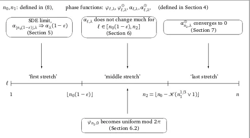
The following figure gives an overview of the main components of the proof.
n0,n1: defined in (8), phase functions: ϕℓ,λ,ϕℓ⊙,λ,αℓ,λ,α⊙ℓ,λ, (defined in Section 4) ✓
✒
✏
✑
SDE limit, α⌊n0(1−ǫ)⌋,λ⇒αλ(1−ǫ)
(Section 5)
✓
✒
✏
✑
αℓ,λdoes not change much for
ℓ∈[n0(1−ǫ),n2]
(Section 6)
☛
✡
✟
✠
α⊙n
2,λ converges to 0
(Section 7)
❄ ❄ ❄
✻
ℓ
1
‘first stretch’ ‘middle stretch’ ‘last stretch’
⌊n0(1−ǫ)⌋ n2=⌊n0− K(n11/3∨1)⌋ n
☛
✡
✟
✠
ϕn2,0becomes uniform mod 2π
(Section 6.2)
4
Phase functions
In this section we introduce the phase functions used to count the eigenvalues.
4.1
The eigenvalue equations
Letsj=pn− j−1/2 and pj =pm−j−1/2. Conjugating the matrix ˜An,m (6) with a(2n)×(2n)
diagonal matrixD=D(n)with diagonal elements
D1,1=1, D2i,2i= χ˜β(pm−i−1)
The first couple of moments of these random variables are explicitly computable using the moment generating function of theχ2-distribution and we get the following asymptotics:
EXℓ=O((m−ℓ)−3/2), EXℓ2=2/β+O((m−ℓ)−1), EXℓ4=O(1),
EYℓ=O((n−ℓ)−3/2), EYℓ2=2/β+O((n−ℓ)−1), EYℓ4=O(1), (30) where the constants in the error terms only depend onβ.
4.2
The hyperbolic point of view
We use the hyperbolic geometric approach of[13]to study the evolution of r andˆr. We will view
R∪ {∞}as the boundary of the hyperbolic plane H={ℑz>0 :z∈C}in the Poincaré half-plane model. We denote the group of linear fractional transformations preservingH by PSL(2,R). The recursions for bothr andˆr evolve by elements of this group of the form x7→b−a/x witha>0.
The Poincaré half-plane model is equivalent to the Poincaré disk modelU={|z|< 1} via the con-formal bijectionU(z) = iz+1
z+i which is also a bijection between the boundaries∂H=R∪ {∞}and
∂U = {|z| = 1,z ∈C}. Thus elements of PSL(2,R) also act naturally on the unit circle ∂U. By lifting these maps toR, the universal cover of∂U, each elementT in PSL(2,R)becomes anR→R
function. The lifted versions are uniquely determined up to shifts by 2πand will also form a group which we denote by UPSL(2,R). For anyT ∈UPSL(2,R) we can look atTas a function acting on ∂H,∂UorR. We will denote these actions by:
∂H→∂H :z7→z.T, ∂U→∂U :z7→z◦T, ∂R→∂R :z7→z∗T.
For everyT ∈UPSL(2,R) the function x 7→ f(x) = x∗T is monotone, analytic and quasiperiodic modulo 2π: f(x +2π) = f(x) +2π. It is clear from the definitions that ei x◦T = ei f(x) and
(2 tan(x)).T=2 tanf(x).
Now we will introduce a couple of simple elements of UPSL(2,R). For a givenα∈Rwe will denote by Q(α) the rotation by α in U about 0. More precisely, ϕ∗Q(α) = ϕ+α. For a > 0,b ∈R we denote byA(a,b)the affine mapz→a(z+b)inH. This is an element of PSL(2,R)which fixes∞ inH and−1 in∂U. We specify its lifted version in UPSL(2,R)by making it fixπ, this will uniquely determines it as aR→Rfunction.
GivenT∈UPSL(2,R), x,y∈Rwe define the angular shift
ash(T,x,y) = (y∗T−x∗T)−(y−x)
which gives the change in the signed distance ofx,yunderT. This only depends onv=ei x,w=ei y and the effect ofTon∂U, so we can also view ash(T,·,·)as a function on∂U×∂U and the following identity holds:
ash(T,v,w) =arg[0,2π)(w◦T/v◦T)−arg[0,2π)(w/v).
The following lemma appeared as Lemma 16 in[13], it provides a useful estimate for the angular shift.
Lemma 12. Suppose that for aT∈UPSL(2,R)we have(i+z).T=i with|z| ≤1
3. Then
ash(T,v,w) = ℜh(w¯−¯v)−z− i(2+4¯v+w¯)z2 i
+ǫ3 = −ℜ[(w¯−¯v)z] +ǫ2=ǫ1,
(33)
where for d=1, 2, 3and an absolute constant c we have
|ǫd| ≤c|w−v||z|d≤2c|z|d. (34)
4.3
Regularized phase functions
Because of the scaling in (11) we will set
Λ =µn+
λ
4n10/2 .
We introduce the following operators
Jℓ=Q(π)A(sℓ/pℓ,µn/sℓ), Mℓ=A((1+Xℓ/pℓ)−1,λ/(4n
1/2 0 pℓ))A(
pℓ
pℓ+1
, 0),
ˆ
Jℓ=Q(π)A(pℓ/sℓ,µn/pℓ), Mˆℓ=A((1+Yℓ/sℓ)−1,λ/(4n1 /2 0 sℓ)).
Then (31) and (32) can be rewritten as
rℓ+1=rℓ.JℓMℓˆJℓMˆℓ, r0=∞.
(We suppressed theλdependence in r and the operatorsM,Mˆ.) Lifting these recursions from ∂H
toRwe get the evolution of the corresponding phase angle which we denote byφℓ=φℓ,λ.
φℓ+1=φℓ∗JℓMℓJˆℓMˆℓ, φ0=−π. (35)
Solving the recursion from the other end, with end condition 0 we get the target phase function φ⊙ℓ,λ:
φℓ⊙=φℓ+⊙1∗Mˆ−ℓ1ˆJℓ−1M−ℓ1J−ℓ1, φ⊙n =0. (36) It is clear thatφℓ,λ andφℓ⊙,λ are independent for a fixedℓ(as functions inλ), they are monotone
and analytic inλand we can count eigenvalues using the formula (21).
In our case bothMℓ andMˆℓ will be small perturbations of the identity soJℓˆJℓ will be the main part
of the evolution. This is a rotation in the hyperbolic plane if it only has one fixed point inH. The fixed point equationρℓ=ρℓ.JℓˆJℓ can be rewritten as
ρℓ=
pℓ sℓ
µn
pℓ − pℓ µ
n sℓ −
1
ρℓ
=
ρℓ(µ2n−p 2
ℓ)−µnsℓ
ρℓµnsℓ−s2ℓ
.
This can be solved explicitly, and one gets the following unique solution in the upper half plane if ℓ <n0+1/2:
ρℓ=
µ2n−m+n 2µnsℓ
+i s
1− (µ
2
n−m+n)2
4µ2 ns2ℓ
. (37)
One also needs to use the identity p2ℓ −s2ℓ =m−nand (12). This shows that ifℓ <n0 thenJℓˆJℓ is
a rotation in the hyperbolic plane. We can move the center of rotation to 0 inU by conjugating it with an appropriate affine transformation:
JℓˆJℓ=Q(−2 arg(ρℓρˆℓ))T
−1
ℓ .
HereTℓ=A(ℑ(ρℓ)−1,−ℜρℓ),XY=Y−1XYand
ˆ
ρℓ=
µ2
n+m−n
2µnpℓ
+i s
1− (µ
2
n+m−n)2
4µ2 npℓ2
In order to regularize the evolution of the phase function we introduce
ϕℓ,λ:=φℓ,λ∗TℓQℓ−1, 0≤ℓ <n0
where Qℓ =Q(2 arg(ρ0ρˆ0))· · ·Q(2 arg(ρℓρˆℓ)) andQ−1 is the identity. It is easy to check that the
initial condition remainsϕ0,λ=π. Then
ϕℓ+1 = ϕℓ∗Q−ℓ−11Tℓ−1JℓMℓˆJℓMˆℓTℓ+1Qℓ
Note that the evolution operator is now infinitesimal:Mℓ,Mˆℓ andT−ℓ1Tℓ+1 will all be asymptotically small, and the various conjugations will not change this.
We can also introduce the corresponding target phase function
ϕℓ⊙,λ:=φℓ⊙,λ∗TℓQℓ−1, 0≤ℓ <n0. (39)
The new, regularized phase functions ϕℓ,λ and ϕℓ⊙,λ have the same properties asφ,φ⊙, i.e.: they
are independent for a fixedℓ(as functions inλ), they are monotone and analytic inλand we can count eigenvalues using the formula (24). (See (22) and the discussion before it.)
We will further simplify the evolution using the following identities:
−ar +b=
This allows us to write
We will introduce the following operators to break up the evolution into smaller pieces:
Lℓ,λ=A(1,λ/(4n1 /2
0 pℓ)), Lˆℓ,λ=A(1,λ/(4n1 /2 0 sℓ)),
Sℓ,λ=L ˆ
Tℓ
ℓ,λ
ˆ
T−ℓ1A( pℓ
pℓ+1
(1+Xℓ/pℓ)−1, 0) ˆTℓ
, (41)
ˆ
Sℓ,λ= ˆLTℓ
ℓ,λ
Tℓ−1A((1+Yℓ/sℓ)−1, 0)Tℓ+1. Then
ϕℓ+1 = ϕℓ∗
LTˆℓ
ℓ
Qˆℓ
Sℓ,0Qˆℓ
ˆ LTℓ
ℓ
Qℓ ˆ
Sℓ,0Qℓ =ϕℓ∗
Sℓ,λQˆℓˆSℓ,λQℓ. (42) We also introduce the relative (regularized) phase function and target phase function:
αℓ,λ:=ϕℓ,λ−ϕℓ,0, αℓ⊙,λ:=ϕℓ⊙,λ−ϕ⊙ℓ,0. (43)
5
SDE limit for the phase function
Let Fℓ denote the σ-field generated by ϕj,λ,j ≤ ℓ−1. Then ϕℓ,λ is a Markov chain in ℓ with
respect to Fℓ. Indeed, the relation (42) shows that ϕℓ+1,λ = hℓ,λ(ϕℓ+1,λ,Xℓ,Yℓ) where hℓ,λ is a
deterministic function depending on ℓ andλ. Since Xℓ,Yℓ are independent of Fℓ it follows that
Eϕℓ+1,λ|Fℓ
= Eϕℓ+1,λ|ϕℓ,λ
. We will show that this Markov chain converges to a diffusion limit after proper normalization. In order to do this we will estimate Eϕℓ+1,λ−ϕℓ,λ|Fℓ
and
E(ϕℓ+1,λ−ϕℓ,λ)(ϕℓ+1,λ′−ϕℓ,λ′)|Fℓ
using the angular shift lemma, Lemma 12.
To simplify the computations we introduce ‘intermediate’ values for the processϕℓ,λby breaking the
evolution operator in (42) into two parts:
ϕℓ+1/2,λ=ϕℓ∗
Sℓ,λQˆℓ, Fℓ+1/2=σ(Fℓ∪ {ϕℓ+1/2,λ}).
Note thatϕℓ,λis still a Markov chain if we consider it as a process on the half integers.
Remark 13. We would like to note that the ‘half-step’ evolution rules ϕℓ,λ →ϕℓ+1/2,λ, ϕℓ+1/2,λ →
ϕℓ+1,λ arevery similar to the one-step evolution of the phase functionϕ in [13]. Indeed, in[13],
the evolution ofϕis of the typeϕℓ+1=ϕℓ∗
˜
Sℓ,λQ˜ℓ where ˜Sis an affine transformation and ˜Qis a rotation similar to ourS,ˆSandQ,Qˆ. In our case the evolution ofϕℓ+1,λ is the composition of two
transformations with similar structure. The main difficulties in our computations are caused by the fact thatQandQˆ are rather different which makes the oscillating terms more complicated.
5.1
Single step estimates
Throughout the rest of the proof we will use the notation k= n0−ℓ. We will need to rescale the discrete time by n0 in order to get a limit, we will uset =ℓ/n0 and also introduceˆs(t) =
p
We start with the identity
Note that this means that
ρℓ = ±
m−nand negative otherwise. For the angular shift estimates we need to consider
Zℓ,λ := i.S−ℓ,1λ−i= have the following estimates for the deterministic parts (by Taylor expansion):
vℓ,λ = where the constants in the error term only depend onβand
q(1)(t) =2ρˆ(t)
Proposition 14. Forℓ≤n0we have
Proof. We start with the identity
ϕℓ+1/2,λ−ϕℓ,λ=ϕℓ+1,λ∗Qˆℓ−1−ϕℓ,λ∗Qˆℓ−1=ϕℓ,λ∗Qˆℓ−1Sℓ,λ−ϕℓ,λ∗Qˆ−ℓ1=ash(Sℓ,λ,eiϕℓ,λη¯ℓρˆ−ℓ2,−1).
Here we used the definition of the angular shift with the fact that Sℓ,λ (and any affine
transfor-mation) will preserve∞ ∈ Hwhich corresponds to −1 in U. A similar identity can be proved for
∆1/2ϕℓ+1/2,λ.
The proof now follows exactly the same as in[13], it is a straightforward application of Lemma 12 using the estimates onvℓ,λ,ˆvℓ,λ,Vℓ,Vˆℓ.
5.2
The continuum limit
In this section we will prove thatϕ(n)(t,λ) =ϕ
⌊t n0⌋,λ converges to the solution of a one-parameter
family of stochastic differential equations on t∈[0, 1). The main tool is the following proposition, proved in[13](based on[11]and[4]).
Proposition 15. Fix T >0, and for each n≥1consider a Markov chain Xℓn∈Rdwithℓ=1, . . . ,⌊nT⌋. Let Yℓn(x)be distributed as the increment Xℓ+n 1−x given Xℓn=x. We define
Suppose that as n→ ∞we have
Assume also that the initial conditions converge weakly, X0n=d⇒X0. Then(X⌊nnt⌋, 0≤t≤T)converges in law to the unique solution of the SDE
d X =b d t+σd B, X(0) =X0, t∈[0,T],
where B is a d-dimensional standard Brownian motion and σ : Rd×[0,T] is a square root of the matrix valued function a, i.e. a(t,x) =σ(t,x)σ(t,x)T.
We will apply this proposition to ϕℓ,λ withℓ≤ n0(1−ǫ) and ℓ∈Z/2, so the single steps of the
proposition correspond to half steps in our setup.
The following lemma shows that the oscillatory terms in the estimates of Proposition 14 average out in the ‘long run’. Its proof relies on Proposition 14 and Lemma 26 of the Appendix.
Lemma 16. Let|λ|,|λ′| ≤λ¯andǫ >0. Then for anyℓ1≤n0(1−ǫ),ℓ1∈Z and the implicit constants inO depend only onǫ,β, ¯λ. The indices in the summation
∼
P
run through half integers.
Proof of Lemma 16. We will only prove the first statement, the second one being similar. Note that bλ(t) =b
(1) λ (t) +b
(2) λ (t).
Summing the first and third estimates in Proposition 14 we get (51) with an error term
where the first two terms will be denotedζ1,ζ2. Here
e1,ℓ=
(−vλ−iq(1)/2) ˆρℓ2+ (−ˆvλ−iq(2)/2)
e−i x, e2,ℓ=i( ˆρ−ℓ4q(1)+q(2))e−2i x/4
where for this proofcdenotes varying constants depending onǫ. Using the fact thatvλ,ˆvλ,q(1),q(2)
and their first derivatives are continuous on[0, 1−ǫ]we get
|ei,ℓ|<c, |ei,ℓ−ei,ℓ+1|<cn−01. (54)
Applying Lemma 26 of the Appendix to the first sum in (53):
|ζ1| ≤
1
n0|e1,ℓ1||F
(1)
1,ℓ1|+
1 n0
ℓ1−1 X
ℓ=1
|e1,ℓ−e1,ℓ+1||F1,(1ℓ)|.
Sinceℓ1≤n0(1−ǫ)we have|F
(1)
1,ℓ| ≤c(1+n
1/2 1 k−
1/2)
≤c(n11/2n0−1/2+1)and
|ζ1| ≤c(n− 3/2 0 n
1/2 1 +n−
1 0 ).
(Recall thatk=n0−ℓ.) For the estimate ofζ2 we first note that |e2,ℓ|=
1 2β
n0 k |ρˆ
−2
ℓ +ρ
2
ℓ|=
1 2β
n0 k |ρˆ
2
ℓρ
2
ℓ +1|. (55)
We will use Lemma 26 if|ρˆℓ2ρ2ℓ+1|is ‘big’, and a direct bound with (55) if it is small. To be more precise: we divide the sum into three pieces, we cut it at indicesℓ∗1andℓ∗2so that
|ρˆℓ2ρ2ℓ+1| ≤n0−1/2 ifk∈[k∗2,k∗1] and|ρˆℓ2ρℓ2+1| ≥n−01/2 otherwise. (56) Note that one or two of the resulting partial sums may be empty. We can always find such indices because argρˆ2ℓρℓ2 is monotone if µn ≥
p
m−n and if µn < p
m−n then argρˆ2ℓρℓ2 decreases if k>pm1n1 then it increases. (See the proof of Lemma 26.)
We denote the three pieces byζ2,i,i=1, 2, 3 and bound them separately. Sincek≥ǫn0, Lemma 26
gives
|ζ2,1| ≤c(n 1/2 1 n
−3/2 0 +n
−1/2 0 ).
The term|ζ2,3| can be bounded exactly the same way, so we only need to deal withζ2,2. Here we
use (55) to get a direct estimate:
|ζ2,2| ≤
1 2β
X
k∈[k2∗,k1∗]∩[ǫn0,n0]
1 k|ρˆ
−2
ℓ +ρ
2
ℓ| ≤cn
−1/2 0 .
Collecting all our estimates the statement follows.
Proposition 17. Assume that m/n0 → κ ∈ [1,∞], n/n0 → ν ∈ [1,∞] and that eventually µn >
p
m−n or µn ≤ p
m−n. Then the continuous functions p(n)(t)−1,ρ(n)(t),ρˆ(n)(t) converge to following limits on[0, 1):
p−1(t) = (κ−t)−1/2, ρ(t) =± r
ν−1 ν−t +i
r
1−t
ν−t, ρˆ(t) = r
κ−1 κ−t +i
r
1−t κ−t,
where the sign inℜρ depends on the (eventual) sign of µn− p
m−n. Ifκ = ∞ then p−1(t) = 0,
ˆ
ρ(t) =1and ifν=∞thenρ(t) =±1.
Let B and W be independent real and complex standard Brownian motions, and for eachλ∈Rconsider the strong solution of
dϕλ =
λ 2ˆs−
ℜρ′
ℑρ +
ℑ(ρ2+ ˆρ2)
2βˆs2 + ℜρˆ
2pˆs
d t+ p
2ℜ(e−iϕλdW)
p
βˆs
+ p
2+ℜ(ρ2+ ˆρ2) p
βˆs
d B,
ϕλ(0) = π. (57)
Then we have
ϕλ,⌊n0t⌋ d
=⇒ϕλ(t), asn→ ∞,
where the convergence is in the sense of finite dimensional distributions forλand in path-space D[0, 1)
for t.
Proof. The proof is very similar to the proof of Theorem 25 in[13]. One needs to check that for any fixed vector(λ1, . . . ,λd) the Markov chain(ϕℓ,λi, 1≤ i≤ d),ℓ≤ ⌊(1−ǫ)n0⌋,ℓ∈Z/2 satisfies the
conditions of Proposition 15 and to identify the variance matrix of the limiting diffusion. Note that because our Markov chain lives on the half integers one needs to slightly rephrase the proposition, but this is straightforward.
The Lipshitz condition (48) and the moment condition (49) are easy to check from Proposition 14. The averaging condition (50) is satisfied because of Lemma 16, using the fact that because of the conditions of the proposition, the functionsbλ(t),a(t,x,y)converge. This proves that the rescaled version of(ϕℓ,λj, 1≤ j≤d)converges in distribution to an SDE inR
d where the drift term is given
by the limit of(bλj,j =1 . . .d)and the diffusion matrix is given by a(t,x)j,k = 2
βˆs2ℜ
ei(xk−xj)+ 2+ℜ( ˆρ2+ρ2)
βˆs2 .
The only step left is to verify that the limiting SDE can be rewritten in the form (57). This follows easily using the fact that ifZis a complex Gaussian with i.i.d. standard real and imaginary parts and ω1,ω2∈Cthen
Eℜ(ω1Z)ℜ(ω2Z) =ℜ(ω¯1ω2).
The following corollary describes the scaling limit of the relative phase functionαℓ,λ.
Corollary 18. Let Z be a complex Brownian motion with i.i.d. standard real and imaginary parts and
consider the strong solutionαλ(t)of the SDE system (17). Thenα⌊n0t⌋,λ d
=⇒αλ(t)as n→ ∞ where
Proof. We just need to show that for any subsequence of nwe can choose a further subsequence so that the convergence holds. By choosing an appropriate subsequence we can assume that m/n0,n/n0 both converge and thatµn−
p
m−nis always positive or nonnegative. Then the con-ditions of Proposition 17 are satisfied andαλ =ϕλ−ϕ0 will satisfy the SDE (17) with a complex
Brownian motionZt:=R0teiϕ0(t)dW
t. From this the statement of the corollary follows.
6
Middle stretch
In this section we will study the behavior ofαℓ,λandϕℓ,λ in the interval[⌊(1−ǫ)n0⌋,n2]withn2= j
n0− K(n11/3∨1) k
. The constantK will eventually go to∞, so we can assume thatK > C0 >0 withC0large enough.
6.1
The relative phase function
The objective of this subsection is to show that the relative phase function αℓ,λ does not change
much in the middle stretch.
Proposition 19. There exists a constant c=c(λ,¯ β)so that with y =n0−1/2(n11/6∨logn0)we have
E|αℓ2,λ−αℓ1,λ| ∧1|Fℓ1
≤cd(αℓ1,λ, 2πZ) + p
ε+y+K−1 (58) for allK >0,ε∈(0, 1),λ≤ |λ¯|,n0(1−ǫ)≤l1≤l2≤n2,ℓ∈Z.
Because of the moment bounds (30) we may assume that
|Xℓ|,|Yℓ| ≤
1 10
pn
0ˆs(ℓ/n0), forℓ≤n2. (59)
Indeed, the probability that (59) does not hold is at most c(n0−n2)−1 ≤ cK−1 which can be
absorbed in the error term of (58).
We first provide the one-step estimates for the evolution of the relative phase function.
Proposition 20. There exists c =c(β, ¯λ)so that for everyℓ≤n2 and|λ|<λ¯ we have the following
estimates
E∆αℓ,λ|Fℓ
=− 1
n0ℜ ¦
ηℓ
e−iϕℓ,λ−e−iϕℓ,0ρˆ−2
ℓ
vλ+iq(1)/2+ˆvλ+iq(2)/2]} − 1
n0ℜ ¦
iη2ℓ/4e−2iϕℓ,λ−e−2iϕℓ,0ρˆ−4
ℓ q
(1)+q(2)]
}+O( ˆαℓ,λk−3/2+k−1/2n−1 /2 0 ) =O( ˆαℓ,λk−1+k−1/2n−01/2) (60)
E∆α2ℓ,λ|Fℓ
=O( ˆαℓ,λk−1+k−1n−01) (61)
E|∆αℓ,λ∆ϕℓ,λ|
Fℓ
=O( ˆαℓ,λk−1) (62)
Proof. We first prove estimates on∆1/2αℓ,λ and∆1/2αℓ+1/2,λ. In order to do this, we break up the
evolution ofϕℓ,λinto even smaller pieces:
ϕℓ,λ
the intermediate steps in the natural way.
By choosingc(β, ¯λ)large enough we can assume λ¯
4pn0k ≤ 1
10forℓ≤n2≤n−K. Using this with the
cutoff (59) the random variablesZℓ,λ,Zˆℓ,λdefined in (46) are both less than 1/3 in absolute value.
This means that we are allowed to use Lemma 12 in the general case for each operator appearing in (63) (i.e. the condition|z| ≤1/3 is always satisfied). From this point the proof is similar to the proof of Proposition 29 in[13]. We first write
∆1/2αℓ,λ = ash(L 12 again for the third term together with
|eiϕℓ,λ−eiϕℓ,0|=|eiαℓ,λ−1| ≤αˆ
this is the analogue of Lemma 32 from[13]and it can be proved exactly the same way. To get (60) we write
The next lemma provides a Gronwall-type estimate for the relative phase function. This will be the main ingredient in the proof of Proposition 19. The proof is based on the single step estimates of Proposition 20 and the oscillation estimates of Lemma 26, the latter will be proved in the Appendix.
Lemma 21. There exist constants c0,c1,c2depending onλ,¯ βand a finite set J depending on n,n1,m1
From Proposition 20 we can write
so we only need to bound the first two terms.
We will use
which is the ‘one-step’ version of (66) and can be proved the same way as Lemma 32 in[13]. From this we get the estimates
|ei,ℓ| ≤c xℓ/k, |∆ei,ℓ| ≤ck−2xℓ+cn−01/2k−3/2. Then by Lemma 26 we have
In order to boundζ2 we use a similar strategy to the one applied in the proof of Lemma 16. We
divide the index set[ℓ1,ℓ2]into finitely many intervals I1,I2, . . . ,Ia so that for each 1≤ j≤ aone
of the following three statements holds:
for eachℓ∈Ij we havek≥pn1m1and|ρˆ2ℓρ most three roots (it is a cubic equation, see the proof of Lemma 26 for details) we can always get a suitable partition with at most five intervals. Moreover the endpoints of these intervals (apart fromℓ1 andℓ2) will be the elements of a set of size at most four with elements only depending on
n,m1,n1.
We will estimate the sums corresponding to the various intervalsIjseparately. IfIjsatisfies condition (69) then we use We can bound the first term as
xℓ∗
Note that the sum of the error terms (71) is
where we used(n11/3∨1)≤k≤n0. Putting our estimates together:
|X
ℓ∈Ij
ℜ(η2ℓe2,ℓ)| ≤cK−1/2xℓ∗
1+c
ℓ∗1−1 X
ℓ=ℓ1
xℓ(k−3/2+ (n1 /3
1 ∨1)k−
2) (72)
+c(n−01/2logn0+ (n11/6∨1)n−01/2). The only case left is when Ij = [ℓ∗1,ℓ∗2] satisfies condition (68). If µn ≥
p
m−n then we have the same estimate for Fℓ(,2ℓ)∗
2
as in (70) so we get exactly the same bound as in (72). If we have
µn< p
m−nthen we use (80) of Lemma (26) with the bound
|Fℓ(2∗)
1,ℓ| ≤
c(k1/2+n11/2(k∗1)−1/2+1). Copying the previous arguments we get
|X
ℓ∈Ij
ℜ(η2ℓe2,ℓ)| ≤ cK−1/2xℓ∗
2−1+c
ℓ∗
2−1 X
ℓ=ℓ∗1
xℓ(k−3/2+ (n11/3∨1)k−2)
+c(n−01/2logn0+ (n 1/6 1 ∨1)n
−1/2 0 ).
Collecting our estimates, noting thatℓ∗2−1 is the endpoint of one of the intervalsIj and lettingK be large enough we get the statement of the lemma.
The proof of Proposition 19 relies on the single step estimates of Proposition 20 and the following Gronwall-type lemma which was proved in[13].
Lemma 22. Suppose that for positive numbers xℓ,bℓ,c, integersℓ1< ℓ≤ℓ2 we have
xℓ≤
xℓ−1 2 +c+
ℓ−1 X
j=ℓ1
bjxj. (73)
Then xℓ2≤2(xℓ1+c)exp
3Pℓ2−1 j=ℓ1 bj
.
Now we are ready to prove Proposition 19.
Proof of Proposition 19. We will adapt the proof of Proposition 28 from [13]. Let a = αℓ1,λ and
define a◊,a◊ ∈ 2πZ so that [a◊,a◊) is an interval of length 2π containing a. We can assume that λ≥0, the other case being very similar. We will drop the index λ fromα and we will write
E(.) =E(.|Fℓ1).
We will show that there existsc0so that ifK >c0, then if ˜a=a♦ora♦then
E|αℓ
2−a˜| ≤ c1(|a−a˜|+ p
ǫ+y). (74)