LI-VANG LOZADA-CHANG
Abstract. In this paper we study asymptotic behavior of some mo-ment spaces. We consider two different settings. In the first one, we work with ordinary multi-dimensional moments on the standardm-simplex. In the second one, we deal with the trigonometric moments on the unit circle of the complex plane. We state large and moderate deviation principles for uniformly distributed moments. In both cases the rate function of the large deviation principle is related to the reversed Kull-back information with respect to the uniform measure on the integration space.
1. Introduction
In this paper we present asymptotic behavior analysis of some moment spaces. We consider multi-dimensional power moments on the m -dimen-sional standard simplex and trigonometric moments on the complex unit circle. To begin with, let us introduce a general setting.
Let L be an infinite set of index and let {φt : t ∈ L} be a family of continuous complex valued functions defined on a bounded setK⊂Ω (with Ω = C⏐ or IRd, d ∈ IN∗). Let (Ln : n ∈ IN∗) be an increasing sequence of finite subsets of L such that nLn = L. For n ∈ IN∗, the n-th moment space is the set
Mn :=
K
Φndµ:µ∈ P(K)
⊂C⏐ #(Ln)
where Φn:= (φt :t∈ Ln), #(A) stands for the cardinality of the setA and
P(K) denotes the set of all probability measures with support included in
K. It is well know thatMnis the convex hull of the curve{Φn(x) : x∈K} [KN77, Theorem I.3.5]. A deeper knowledge of the shape and structure of these spaces is one of the byproducts of our results. The set P(K) will be endowed with the weak topology [Bil99].
For n, k ∈ IN∗ such that n ≥ k, let Πn,k : C⏐#(Ln) → C⏐#(Lk) be the natural projection map. Let (Mn:n∈IN) be a sequence of sets verifying
Mn⊂Mn⊂C⏐#(Ln) (n∈IN∗), (1.1a) Πn,kMn⊂Πn+1,kMn+1, (n, k∈IN∗, k≤n) (1.1b)
n≥k
Πn,kMn=Mk (k∈IN∗). (1.1c)
Date: May 5, 2004.
1991 Mathematics Subject Classification. Primary: 60F10, 44A60 Secondary: 42A70.
Key words and phrases. Random Moment Problem, Large Deviations, Multidimen-sional Moment, Kullback information, reversed Kullback information.
The setsMncould be seen asextended moment spaces. By (1.1c), these sets provide good approximation of moment spaces. In general, is not possible to have a tractable description of the moment spaces. Nevertheless, by means of the approximating sets Mn (easily describable) we will be able to deal with the asymptotics of moment spaces.
Assuming that it is feasible, we endow Mn with the uniform probability measure Un, i.e. with the corresponding normalized Lebesgue measure. Let
k be a fixed integer, we focus on the asymptotic behavior of the first k -dimensional marginal probability ofUn. More precisely, letXn be a random vector ofMnwith distributionUn. We aim to find convergence rates (in the sense of large deviations) for the sequence of random vectors
Xnk:= Πn,kXn.
Up to our knowledge, this problem was first studied in [CKS93]. Therein, the authors deal with the ordinary power moments on [0,1]. They consider the moment spaces
Mn=
1
0
Φndµ:µ∈ P([0,1])
with Φn(x) = (x, x2, ..., xn). Endowing Mn with the corresponding uni-form probability measure they show that (Xk
n :n ∈ IN) converges toc0 =
(c01, c02, ..., c0k), the k-dimensional moment vector of the arc-sine law on [0,1], i.e.
c0j =
1
0
xj
πx(1−x)dx (j = 1,2, ..., k).
Moreover, they obtain that the limit distribution of the fluctuations is nor-mal. More precisely,
√
n(Xnk−c0)−−−→Law
n→∞ Nk(0,Σ),
where Σ is a matrix whose coefficients depend on the arc-sine law moments. In the same framework the large and moderate deviations behavior are studied in [GLC]. The main result is that, for any borelian set A of [0,1],
IP Xnk∈A≈exp (−ninf{I(x) :x∈A})
whereI is a convex function related to the reverse Kullback information with respect to arc-sine law (See Section 2.2 for the definition of this functional). Here, ≈ stands for large deviation equivalence (See Section 2.1 for right formulation). The large deviation principle (LDP) is also stated for the (random) upper representation probability measures of the random vectors
Xn, (n∈IN).
In this paper we focus on two different settings. The first one concerns the m-dimensional power moments on S (with m positive integer). The standard m-simplex is the set
S :=
(x1, x2, ..., xm)∈IRm+ :
m
i=1
xi≤1
For β= (β1, β2, ..., βm)∈INm, define
φβ(x) =xβ11 xβ22 · · ·xβmm. (1.2) Let
Ln:=
(β1, β2, ..., βm)∈INm: 0< n
i=1
βi ≤n
(n∈IN)
and
ΦSn =φβ:β ∈ Ln
.
The n-th moment space (onS) is
MnS:=
S
ΦSndµ:µ∈ P(S)
.
The second setting involves the trigonometric moments on TT, the unit circle of C⏐ . The moment spaces are
MnTT:=
TT
zjdµ(z) : 1≤j≤n
:µ∈ P(TT)
(n∈IN).
Theorem 2.2 of [Gup99b] state that an infinite multi-sequence is a mo-ment multi-sequence if and only if it is completely monotone. Taking for all n ∈ IN∗, Mn as the set of all partially monotone multi-sequence of order n, denoted by Gn, the conditions (1.1) are fulfilled (See Definition (3.1) and Theorem (3.2) for details). In [Gup00] a normal central limit for
Xnk : n ∈ IN is shown. The central role played by the arc-sine law in [CKS93] and [GLC], is in this case played by νS, the uniform probability
measure on S. In Section 4, in the context of the trigonometric moment, we obtain the convergence of the random moment vector sequence (Xk
n) to the moment vector of νTT, the uniform probability measure on TT, and its limit distribution (after normalization).
One of our main results is the statement of the large deviation principle (LDP) for (Xk
n:n∈IN) in both settings. Using the symbolKto represent
S or TT our result can be written as follows. For sake of simplicity we drop the index Kof Xk
n andLn.
IP Xnk∈A≈exp (−#(Ln)I(A)) (Ameasurable set) where
IK(A) = inf µ∈ P(K,A)
K ln
dνK dµ
dνK
, (1.3)
and
P(K, A) :=µ∈ P(K) :
K
ΦKk dµ ∈A.
Throughout the paper we follow the convention that the infimum over an empty set is +∞.
This last result, as in [GLC], leads to obtain the useful expression for I(.) as in (1.3).
The paper is organized as follows. To be self contained in next section we recall some definitions and basic results on large deviation and Kullback in-formation. In Section 3 and 4 we state our results for the multi-dimensional and trigonometric moment setting respectively. Section 5 is devoted to com-paring our result with the previous one in [GLC]. The proofs of all results are deferred to the last sections.
2. Large Deviations and Kullback Information
2.1. Large Deviation Principle. Let us first recall what a LDP is (see for example [DZ98]). Let (un) be a positive sequence of real numbers decreasing to 0.
Definition 2.1. We say that a sequence (Rn) of probability measures on a measurable Hausdorff space (U,B(U)) satisfies a LDP with rate function I
and speed (un) if:
i) I is lower semicontinuous, with values in IR+∪ {+∞}. ii) For any measurable setA of U:
−I(intA)≤lim inf
n→∞ unlogRn(A)≤lim supn→∞
unlogRn(A)≤ −I(cloA),
whereI(A) = infξ∈AI(ξ) and intA(resp. cloA) is the interior (resp. the closure) of A.
We say that the rate function I is good if its level sets{x ∈U : I(x)≤a}
are compact for any a≥0. More generally, a sequence of U-valued random variables is said to satisfy a LDP if their distributions satisfy a LDP.
To be self-contained let us recall some facts and tools on large deviations which will be useful in the paper (we refer to [DZ98] for more on large deviations).
• Contraction principle. Assume that (Rn) satisfies a LDP on (U,B(U)) with good rate function I and speed (un). Let T be a continuous mapping from U to another space V. Then, (Rn◦T−1) satisfies a LDP on (V,B(V)) with good rate function
I′(y) = inf
x:T(x)=yI(x), (y∈V), and speed (un).
• Exponential approximation. Assume that U is a metric space and letddenotes the distance onU. Let (Xn) be aU-valued random sequence satisfying a LDP with good rate functionI and speed (un). Let (Yn) be anotherU-valued random sequence. If for anyξ >0
lim sup
n→∞ unlog IP(d(Xn, Yn)> ξ) =−∞,
then (Yn) satisfies the same LDP as (Xn).
speed (vn) we say that (Xn) satisfies a moderate deviation principle (MDP) [DZ98].
2.2. Kullback and Reversed Kullback Information. Let µ and ν be probabilities on certain measurable space U. The Kullback information or cross entropy of µwith respect to ν is defined by
K(µ, ν) =
⎧ ⎨ ⎩
U ln dµ
dν dµ, ifµ≪ν and ln
dµ
dν ∈L1(µ) +∞, otherwise.
(2.1)
Properties of K as a function of µ may be found in [Bre79]. K(·, ν) is the rate function for Sanov large deviations theorem (see Section 6.2 of [DZ98]) where ν is a probability generating the random variables. In this paper, the rate function involved is the reversed Kullback information. This means that we will consider K in (2.1) as a function of ν. The role of µ will be played by νS (resp. νTT) for the multi-dimensional (resp. trigonometric)
moment setting.
In order to identify the rate function that controls the LDP in the multi-dimensional moment framework (Lemma 6.3) we exploit an optimization result on measure space [BL93, Theorem 3.4]. Namely, this result establish the duality relation between an optimization problem on measure space and the corresponding dual optimization problem on continuous function space. For the Kullback information (defined for general Borel measures), this relation can be paraphrased as follows. For x∈IR#(Lk),
inf
K(ν, µ) +µ(U) : µregular Borel finite measure,
U
Φkdµ=x
= sup
Λ, x+
U
ln(1− Φk,Λ) dν : Λ∈IR#(Lk)
where·,· denotes the usual scalar product in IR#(Lk). We refer the reader to [BL93] for general statement and related results.
3. Multidimensional moment problem We recall themulti-dimensional moment space of ordern
MnS :=
cβ=
S
xβdµ(x) :β∈ Ln
:µ∈ P(S)
where xβ := xβ1
1 xβ22 ...xβmm (with 00 = 1) for x = (x1, x2, ..., xm) ∈ IRm and β= (β1, β2, ..., βm)∈INm. Forβ∈INm, let |β|:=mi=1βi.
Definition 3.1. A multi-sequence (cβ : |β| ≥ 1) is called a completely monotone multi-sequence if for all β0 ∈IN and β∈INm
(−1)β0∆β0cβ≥0 (3.1)
where, with c(0,0,...,0)= 1,
∆cβ=c(β1+1,β2,...,βm)+c(β1,β2+1,...,βm)+...
+c(β1,β2,...,βm+1)−cβ
(∆β0 stands for β0 iterates of the operator ∆). A finite multi-sequence
allβ0∈IN andβ∈INmsuch thatβ0 ≤n−|β|(3.1) holds. Following [Gup00]
we will call the completely (resp. partially) monotone multi-sequences asG -sequences (resp. partial G-sequences).
The G-sequences are the multi-dimensional version of the completely monotone sequences on IR. These sequences are the solution of the Haus-dorff moment problem, i.e. the power moment problem on [0,1] [ST63]. The following theorem, due to [Gup99a], solves the multi-dimensional moment problem on S.
Let R∞be the set of all infinite real multi-sequences. We recall that L =
n
Ln= INm\ {(0,0, ...,0)}.
Theorem 3.2 (Theorem 2.2 [Gup99a]). Letc = (cβ:β∈ L)∈ R∞. There exists µ∈ P(S) such that
cβ=
S
xβdµ(x) (∀β∈ L).
if and only if c is aG-sequence.
We denote by Rn the set of all multi-sequence of order n, i.e. Rn = IR#(Ln). For n, k ∈ IN∗ with k < n, let ΠS
n,k : Rn → Rk (n ≥ k) be the projection map defined as
(cβ:β∈ Ln)→(cβ:β∈ Lk).
Let Gn denote the set of all partial G-sequences of order n. Thus, by the previous theorem MS
k ⊂ΠSn,k(Gn)⊂ΠSn+1,k(Gn+1) for alln > k. Moreover,
MS
k =
n≥kΠSn,k(Gn).
The sets Gn are completely described in [Gup00]. In particular, they are bounded with nonzero Lebesgue measure . So, we can endow them with the corresponding uniform probability measure. Let XS
n be a random vector of Gn having uniform distribution. We define the random multi-sequence (XnS,k :n∈IN∗) of Gk by
XnS,k:= ΠSn,kXnS.
As we have said in the introduction νS, the uniform distribution on S
plays a major role in the asymptotic behavior of XnS,k : n ∈ IN. Let
cS,k = (cSβ:β ∈ Lk) denotes the moment multi-sequence of order k of νS,
i.e.
cSβ:=
S
xβdνS(x) = m!
m i=1βi
(m+|β|)! (β∈ Lk).
In [Gup00] it is established the following normal central limit for XnS,k.
Theorem 3.3 (Theorema 3.4 [Gup00]).
n+m
n XS
,k n −cS,k
Law −−−→
n→∞ Nk(0,Σ S
k), where
ΣkS =cSγ+β
Our first result concerns the large deviation behavior of the sequences of random multi-sequences XnS,k.
Theorem 3.4. The random vector sequence XnS,k :n∈INsatisfies a LDP with speed n+nm−1 :n∈IN and good rate function
ISk(x) = inf
µ∈ P(S,{x})K(ν
S, µ), (x∈ R
k).
Remark 1. Using the dual relation in Section 2.2 the rate functionISk could be expressed as, for x∈MS
k,
ISk(x) = sup
(Λ0,Λ)∈IR×Rk ⎧ ⎨
⎩Λ0−1 +x,Λ+
S
ln
1−Λ0−
β∈Lk
Λβxβ
dνS(x)
⎫ ⎬ ⎭
The following result gives an estimation of convergence rate between those of the Theorem 3.3 and Theorem 3.4.
Theorem 3.5. Let Mn : n ∈ IN) be a sequence of positive real numbers growing to +∞ such that Mn=o n+nm. The sequence of random vectors
XnS,k :=
n+m n
M(n)
XnS,k−cS,k
satisfies the LDP with speed (M(n)−1) and good rate function
HS(x) := 1 2x
T ΣS
k
−1
x, (x∈ Rk).
Finally, we present LDP in an infinite dimensional setup. Let MS
∞ be the
set of all moment multi-sequences, i.e. in view of Theorem 3.2, the set of all
G-sequences. Take on R∞ the norm defined by
c:= β∈L
1
|β|+m m
|β|2|cβ|, c = (cβ:β∈ L)
. (3.2)
Equip R∞ with the corresponding borelian σ-field. Endow M∞S with the
induced topology and σ-field. Further, let C∞⊂ R∞ defined as
C∞:={c ∈ R∞:∀β 0≤cβ≤1}.
Obviously, M∞S ⊂ C∞. It is well known that the moment problem on S
is determined [ST63, Corollary 1.1]. In others words, given c ∈ MS ∞ there
exists an unique probability measure µc verifying
cβ=
S
xβdµc(x) (∀β∈ L).
For n∈IN∗, let ΠS∞,n:R∞→ Rn be the projection map.
Theorem 3.6. Let (µn) be a sequence of probability measures defined on
C∞ such that
is the uniform probability measure on Gn. Then, (µn) verifies the LDP on
R∞ endowed with the topology induced by the norm (3.2). The good rate function is
IG(c) =
K(νS, µc), if c ∈M∞S,
+∞, otherwise (3.3)
and the speed is n+nm−1 :n∈IN.
Remark 2. As can be seen in the proof of this theorem, it remains valid if we consider as C∞ any bounded set (in the infinity norm) containing MS
∞.
Furthermore, the theorem holds for the family of norms
cl:=
β∈L 1
|β|+m m
|β|l|cβ|, c= (cβ:β∈ L)
with l >1. (3.2) corresponds to the casel= 2.
4. Trigonometric moment problem For µ∈ P(TT) the trigonometric moments on TT are given by
tk(µ) =
TT
zkdµ(z), k∈ZZ.
Since tk(·) = t−k(·) it suffices to consider k ≥ 0 in order to study the corresponding moment spaces. We recall that the (n-th) moment space is
MnTT =tn:= t1(µ), t2(µ), ..., tn(µ):µ∈ P(TT)
.
For z= (z1, z2, ..., zn)∈⏐Cn, let
Tn(z) :=
⎛ ⎜ ⎜ ⎜ ⎝
1 z1 z2 . . . zn ¯
z1 1 z1 . . . zn−1
..
. ... ... ... ¯
zn z¯n−1 z¯n−2 . . . 1
⎞ ⎟ ⎟ ⎟ ⎠.
We denote by ∆n(z) the determinant ofTn(z). Forµ∈ P(TT), the matrices
Tn(µ) :=Tn(tn(µ)),n∈IN∗ are calledToeplitz matrices. They play a major role in the theory of moments on TT.
Let XTT
n be a random vector of MnTT uniformly distributed. Let ΠTn,kT denotes the projection map from C⏐n to C⏐k (k ≤ n). Let XTT,k
n be random vector of MTT
k defined as
XnTT,k := ΠTn,kT XnTT.
Our first result give the limit distribution of √nXnTT,k:n∈IN∗. Conse-quently, we obtain a weak law of large numbers for XnTT,k. Namely,
XnTT,k−→IP
n (0,0, ...,0)∈C ⏐ k.
Note that, for all j∈IN∗,tj(νTT) = 0.
Theorem 4.1. For any measurable set A of C⏐k, lim
n→∞IP( √
n XnTT,k ∈A) = 1
πk
A
exp −z2dρ1(z)
where · denotes the Euclidean norm on C⏐k.
Remark 3. In others words, the limiting distribution of √n XnTT,k :n∈INis ak-dimensional complex normal distribution. Each component are pairwise independent with independent real and imaginary part following normal distribution of expectation zero and variance 1/2. As we see in previous section (and in [CKS93]) the variance of the limiting distribution are very related with the moments of the limit probability. In fact, in this case, as the variance is the identity matrix it is hidden its relation withνTT. A more descriptive formulation of the previous theorem could be
√
nXnTT,k−−−→Law
n→∞ N
C
k (0,Tk(νTT)) where NC
k (·,·) denotes thek-dimensional complex normal distribution. An interesting byproduct of the proof of this theorem is the “asymptotic” volume of n-th moment space. Similar results are given in [CKS93] and [Gup00]. Here, we will obtain that
V olumeIR2n MnTT= πn
n!. (4.1)
Since the Stirling’s expressionn! =√2πnexp(−n)nn+1/2(1 +o(1)), we have
V olumeIR2n MnTT
= exp(−nlnn[1 +o(1)]).
Our next results concern the large and moderate deviation behavior of the sequence XnTT,k :n∈IN.
Theorem 4.2. XnTT,k : n ∈ IN satisfies the LDP with speed n−1 and good rate function
ITkT(z) =
−ln ∆k(z)
∆k−1(z) if z∈intM
TT
k ,
+∞ otherwise. (4.2)
Theorem 4.3. Let(un) be a given decreasing sequence to0such thatn−1 =
o(un). Then √nunXnTT,k :n∈IN satisfies a LDP onC⏐ k with speed un and good rate function
HTT(z) :=
k
j=1
z2j.
Finally we give a LDP for random probability measures. This result follows from Theorem 4.2 and make possible to understand the rate function in (4.2). For everyn, let Q⏐nbe a probability measure defined onP(TT) such that ifµnhas distribution Q⏐nthen the random vectortn(µn) has distribution IPn.
Theorem 4.4. (µn) satisfies a LDP on P(TT) with good rate function
Remark 4. There is a natural way to obtain such Q⏐n. For n ∈ IN∗ and
z ∈ MnTT, let Wz
n be a probability distribution on P(TT,{z}). The mixture probability measure defined as
Q ⏐
n(·) =
MTT
n
Wzn(·) dIPn(z)
verifies our constraint. In [GLC], in the frame of the power moment problem on [0,1], the authors considered for Wz
n the probability measure concen-trated on the upper canonical representation of the moment vector z. See [KN77] for definition. Applying the contraction principle, we obtain
Corollary 4.5.
ITkT(z) = inf
µ∈ P(TT,{z})K(ν
TT, µ).
5. Related LDPs.
The results on LDP obtained in previous sections can be seen in a com-mon frame: the interval [0,1]. We will compare each of these LDP with the previous one obtained in [GLC]. This analysis will give a first approach to a slight generalization of our formulation of the asymptotics analysis on mo-ment spaces. In particular, endowing Mn (or Mn) with general probability measures instead of the uniform one.
5.1. The general [a, b]-moment spaces. We recall briefly certain aspects developed in [CKS93] and [GLC]. First, we want to remark that the all results obtained there are valid if one consider any real bounded interval of the real line. Moreover, the results are valid if one consider the moments associated to a given sequence of polynomial P = (Pn) with degPn = n,
n ∈ IN∗ instead of the ordinary power moments. For any interval [a, b] (a < b) of the real line and n∈IN∗, then-th moment space is
Mk[a,b](P) =('c1(µ),'c2(µ), ...,'ck(µ))∈IRk: µ∈ P([a, b])
.
where, for µ∈ P([a, b]) and j∈IN∗,
' cj(µ) =
b
a
Pj(x) dµ(x).
The reason of the extensibility of the result on [0,1] to any interval [a, b] and any family {Pn} is explained by the canonical moments which are defined as follows. Given 'cj = ('c1,'c2, ...,'cj)∈intMj[a,b](P) we define, forj ∈IN,
c+j+1('cj) = maxc∈IR : (('c1,c'2, ...,'cj, c)∈Mj[a,b+1](P)
c−j+1('cj) = minc∈IR : (('c1,c'2, ...,'cj, c)∈Mj[a,b+1](P)
.
For i∈IN∗, thei-th canonical moment is defined as
'
pi('ck) =p'i('ci) = 'ci−c
−
i ('ci−1)
c+i ('ci−1)−c−
i ('ci−1)
The canonical moments are independent of the particular choice of the se-quenceP[CKS93]. Furthermore, they are invariant by linear transformation (with positive slope) of the support interval. Namely, if µ∈ P([0,1]) is lin-early transformed measure with positive slope to µ′ ∈ P([a, b]), then their corresponding canonical moments are the same [Ski69, Theorem 5]. These properties make very attractive the study of the canonical moments. We refers the reader to [DS97], a very complete monograph about the subject. The results of [CKS93] and [GLC] were based on the knowledge of the exact distribution of the canonical moments. Theorem 1.3 of [CKS93] establish that the uniform probability measure on Mn[a,b](P) (n∈ IN∗) is equivalent to the first ncanonical moment are independent andp'j hasβ(n−j, n−j )-distribution,j = 1,2, ..., n.
5.2. Deriving LDPs on IR from LDP of Section 4. We denoted by
F : TT→[−1,1] the map defined as z→ ℜz. For µ∈ P(TT), let
µF :=µ◦F−1∈ P([−1,1]). (5.1) For k∈ IN∗, let F'k be the application from MkTT to Mk([−1,1]) defined by (5.1). More precisely, for z∈MkTT,
'
F(z) ='ck(µF) := ('c1(µF),c'2(µF), ...,'ck(µF))∈Mk([0,1]),
whereµis any measure onP(TT) representingz. We will see in the following that this application is independent of the selection of µ. Hence, it is well-defined. For j= 0,1, ..., k
ℜtj(µ) =ℜ
TT
zjdµ(z)
=
TT
cos(jarccosF(z)) dµ(z)
=
1
−1
Tj(x) dµF(x)
where Tj = cos(jarccosx) is the j-th Tchebycheff polynomial of the first kind. These polynomials can be expressed as Tj(x) =mj=0amjxj where
amj =
⎧ ⎨ ⎩
m
22
j(−1)m2−j
m+j
j+ 1
if m−j is even,
0, otherwise .
Therefore, for µ∈ P([−1,1]) and fors= (s0, s1, ..., sk) with
sj =sj(µ) :=
1
−1
Tjdµ, j= 0,1, ..., k,
and c= (1,'c1(µ),'c2(µ), ...,c'k(µ)) we havec=A−1s withA= (amj :m, j = 1,2, ..., k). Thus, the relation (1,F'(z)) = A−1(1,ℜz) define F'(·)
indepen-dently of the measure representing z.
By the contraction principle and the δ-method can be derived from the results of Section 4 the asymptotic behavior of sequences of random vectors
'
Zn(k):=F'(XnTT,k) = ΠSn,kF'(Z'n(k)).
to prove that the uniform probability measure onMnTT yields that the firstn
(random) canonical momentsp'j (related toF'(XnTT,n)) are independent with
β(n−j+ 1/2, n−j+ 1/2)-distribution, j= 1,2, ..., n. Compare this result with the corresponding one in previous section.
We can use the asymptotics results to study a moment space on an interval of the real line in different way. Actually, this is an equivalent form of the same study. Consider in the interval [−π, π) the system of continuous functions
Φ[n−π,π):= cosθ,sinθ, cos 2θ, sin 2θ, ..., cosnθ,sinnθ, (n∈IN∗).
For µ ∈ P([−π, π)) the corresponding real trigonometric moments are de-fined as α0 = 1,
αk(µ) =
π
−π
coskθdµ(θ), βk(µ) =
π
−π
sinkθdµ(θ), (k∈IN).
The moment space Mn[−π,π) is defined as
Mn[−π,π)=(α1(µ), β1(µ), ..., αn(µ), βn(µ))T ∈IR2n:µ∈ P([−π, π))
.
We may identify the set P(TT) with P([−π, π)) by the relation z = exp(iθ), forz∈TT andθ= [−π, π). Using the convention dµ(θ) := dµ(eiθ), we have
tk(µ) =
π
−π
eikθdµ(θ), k∈IN.
The power moments tk are related with the trigonometric moments in the following way:
tk(µ) =αk(µ) +iβk(µ).
forµ∈ P(TT) andk∈IN. Taking IPnonMnTT is equivalent to endow the set
Mn[−π,π) with the corresponding uniform probability measure. Therefore, this problem is into the general setting described in the introduction of papers. Moreover, all the results for the random power moment problem on TT can easily translate for the random real trigonometric moments problem on [−π, π). The normal limit can be translate using a δ-method [VdV98] and the large deviations by the contraction principle. In particular, we can formulate the following result.
Let T'n be a random vector of Mn[−π,π) uniformly distributed. LetT'nk be the random vector of Mk[−π,π) formed as projection ofT'n onMk[−π,π).
Corollary 5.1. The sequence of random vectors 'Tnk satisfies a LDP with speed (2n)−1 and good rate function
I[k−π,π)(x) = inf
µ∈ P([−π,π),{x})K
ν[−π,π), µ,
1
0 c1 1
c2
cu
ca
M2
[image:13.612.162.424.62.314.2]1
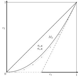
Figure 1. The moment space M2, region limited by the
solid line and the approximating spacesG2, ΠS8,2G8limited by
the segment with extreme points (0,0) and (1,1) (represented in solid line) and the dotted polygonal and dashed polygonal respectively. ca andcu the 2-dimensional moments of arcsine and uniform distribution respectively.
5.3. LDP for one-dimensional G-sequences. Consideringm= 1, in the Section 3 we have an LDP involving ordinary power moments on [0,1].
In [Gup00] the description of the setsGn, (n∈IN∗) is given. In particular, form= 1, the set Gn is the convex hull of the finite set of n+ 1 points
cin= (cin,1, cin,2, ..., cin,n), i= 0,1, ..., n,
with
cin,j =
⎧ ⎪ ⎨ ⎪ ⎩
j i
n i
ifi≤j
0 otherwise,
(j= 0,1, ..., n).
In Figure 1 we sketch the moment spaceM2 and the sets ΠSn,2Gn,n= 2,8. We highlight the points ΠS8,2ci8, i= 0,1, ...,8. As can be seen in the figure the “enlargement” of the extended moment spaces under the curve {x, x2 :
x∈[0,1]} yields that the point limit cu be “underneath” to the pointca.
(µn)⊂ P([0,1]) satisfying the LDP with rate functionIC. Equip [0,1]n(the
n-th canonical moment space) with
µn:=µn⊗µn−1⊗ · · · ⊗µ1∈ P([0,1]n).
Let Πn,k denote the projection map from [0,1]n to [0,1]k, taking the firstn components. Following similar arguments to those of [GLC] (and Section 7 in the context of complex moments) we have that µk
n:=µn◦(Πn,k)−1 :n∈ IN verify the LDP with good rate functionIk
C(p1, p2, ..., pk) =ki=1IC(pi). Letpndenote the application that transforms then-dimensional ordinary moment vector on the corresponding n-dimensional canonical moment vec-tor. Let U'n :=µn◦p−n1. The sequence (ˆµ
(k)
n := U'n◦(Πn,k)−1)⊂ P(Mn[a,b]) satisfy the LDP with Ik(c) =ICk(pk(c)), wherec∈Mk[a,b].
Similar constructions could be make in the complex canonical moment spaces. In a forthcoming paper we will develop these ideas.
6. Proofs of Results of Section 3
6.1. Notation and previous results. We will use the notation of [Gup00]. For β= (β1, β2, ..., βm)∈INm and α= (α1, α2, ..., αm)∈INm,
β! := m
)
i=1
βi!,
n β
:= n!
β!(n− |β|)!,
α β
:= m
)
i=1
αi
βi
,
Nn:= #(Ln) =
n+m
m
−1.
For n∈IN,
Ln:=Ln∪ {(0,0, ...,0)}
and Rn = IR#(Ln), i.e,Rn is the set of the multi-sequences of order n with an additional component indexed by (0,0, ...,0). In this section, for sake of simplify of notation Xnk stands for XnS,k.
Proposition 3.3 of [Gup00] gives a useful expression for the distribution of Xnk. This result is the core of all the proofs. Let (Eα : α ∈ Ln) be a multi-sequence of i.i.d. standard exponential random variables on a certain probability space.
Lemma 6.1. The law of Xnk is same as law of
Yn,β:=
δ∈Ln−|β|
β
+δ δ
Eβ+δ
n β
δ∈Ln Eα
6.2. Proof of Theorem 3.4. LetY'n:n∈IN
be the random finite multi-sequence of Rk defined by
' Yn,β:=
1
N(n)
α∈Ln
1
nα β
Eα (β∈ Lk).
The proof of theorem is based on the LDP for the sum of weighted random variables. In this case, it is not possible to derive it directly from the LDP for weighted empirical means obtained in [GG97], but we may use the result of [Naj02].
From Theorem 2.2 of [Naj02] we have the LDP for the sequence (Xn) with good rate function
I1k(x) = sup
Λ∈Rk
Λ, x+
S
ln(1−PΛ) dνS
, (x∈ Rk),
where, for Λ∈ Rk,PΛ is the polynomial on S
PΛ(x) =
β∈Lk
Λβxβ.
Define the random finite multi-sequence (Yn)
Yn,β :=
α∈Ln:α≥β α β Eα n β Nn
(β∈ Lk). (6.1)
Consider on Rk the following metric d(x,y) :=
β∈Lk
|xβ−yβ|, (x,y∈ Rk) compatible with the topology on it.
Lemma 6.2. The sequences (Y'n) and (Yn) are exponentially equivalent on (Rk,d).
Proof. Letǫ >0. Set
Lǫ,n={α∈ Ln:∀i αi≥ ⌊ǫn⌋},
where⌊w⌋ denotes the biggest integer lower thanw. Fornbig enough such that k < ǫn and for α∈ Lǫ,n
α β n β ≥ m ) i=1 αi−βi
n βi ≥ 1 nα β
1− k ǫn k and α β n β ≤ m ) i=1 α i
n− |β| βi
≤ 1
nα β
1 + k
n−k k
. (6.2)
These two inequalities leads to
1− k ǫn
k
−1≤
α β n β − 1 nα β ≤
1 + k
n−k k
If we set
Q0(ǫ, n) := max
*
1−
1− k ǫn
k
,
1 + k
n−k k −1 + (6.4) then , , , , , α β n β − 1 nα β,, , ,
,≤Q0(ǫ, n)→0 whenn→ ∞.
On the other hand, we have
#(Lǫ,n) = #-(⌊ǫn⌋,⌊ǫn⌋, ...,⌊ǫn⌋) +δ:δ∈ Ln−[ǫn]
.
=N(n− ⌊ǫn⌋).
By straightforward calculations
1−ǫ
1 +m/n m
≤ #(Lǫ,n) N(n) ≤
1−ǫ+m
n m
. (6.5)
For nbig enough, by (6.2), (6.3) and (6.4) we have the bound
d 'Yn,Yn≤ 1
N(n)
⎛
⎝2
α∈Ln\Lǫ,n
Eα+Q0(ǫ, n)
α∈Lǫ,n Eα
⎞ ⎠
Using (6.5) and the fact that #(Ln\ Lǫ,n) =N(n)−#(Lǫ,n),
d 'Yn,Yn≤2
1−
1−ǫ
1 +m/n m
1 #(Ln\ Lǫ,n)
α∈Ln\Lǫ,n Eα
+Q0(ǫ, n) (1−ǫ+m/n)m
1 #(Lǫ,n)
α∈Lǫ,n Eα.
For all Q1 >0, there exists ǫ >0 such that for all nbig enough
2
1−
1−ǫ
1 +m/n m
< t
2Q1
and
Q0(ǫ, n)
1−ǫ+m
n m
< t
2Q1
.
Therefore
IPd 'Yn,Yn> t
≤IP
⎛
⎝ 1
#(Ln\ Lǫ,n)
α∈Ln\Lǫ,n
Eα> Q1
⎞ ⎠
+ IP
⎛
⎝ 1
#(Lǫ,n)
α∈Lǫ,n
Eα> Q1
⎞ ⎠.
(6.6)
By the LDP for empirical mean of independent standard exponentially distributed random variables (particular application of Cram´er’s Theorem [DZ98, Theorem 2.2.3]), follows
lim n
1
nln IP * 1 n n i=1
Zi ≥Q1
+
Hence, by Lemma 1.2.15 of [DZ98], (6.5) and (6.6)
lim sup 1
N(n)ln IP
d 'Yn,Yn> t
≤maxǫ(1 + lnQ1−Q1),(1−ǫ)(1 + lnQ1−Q1)
≤1 + lnQ1−Q1
The exponentially equivalence is then consequence of the arbitrariness of t
and Q1.
By the previous lemma Yn verifies the same LDP as 'Yn. The con-traction principle with the continuous application fromRkto Rk defined by (xβ:β∈ Lk)→ xβ/x(0,0,...,0) :β∈ Lk
yields the LDP for
Yn,β=
Yn,β
Yn,(0,0,...,0)
, (β∈ Lk).
Therefore, in view of Lemma 6.1, Xnkverifies a LDP with good rate func-tion
I2k(x) := inf y∈Rk
I1k(y) : yβ
y(0,0,...,0)
=xβ,β∈ Lk
.
It remains to proof that Ik
S≡I2k.
Lemma 6.3. Ik
S ≡I2k.
Proof. The core of the proof is a particular application of a duality theorem concerning optimization on measure spaces. Let M(S) (resp. M+(S))
be the space of all Borel finite (resp. finite positive) measures on S. By Theorem 7.1.3 of [Dud89] the set M(S) coincide with the set of all regular Borel finite measures on S. Forµ∈ M(S), letµ=µa+µσ be the Lebesgue decomposition of µrespect to νS. Let
Υ1(µ) :=−
S
ln
dµa dν
dνS+∞ ·µ−σ(S), µ∈ Mr(S),
Υ2(Λ) :=
S
ln (1−PΛ) dνS−1, Λ∈ Rk.
From Theorem 3.4 of [BL93], for x∈ Rk, inf
µ∈M(S,x){Υ1(µ) +µ(S)}= supΛ∈Rk{x,Λ+ Υ2(Λ)}, (6.7)
where, for x∈ Rk,
M(S, x) :=
µ∈ M(S) :
S
yβdµ(y) =xβ,β∈ Lk
.
If µ /∈ M+(S), then either µ−σ(S) > 0 or νS
dµa
dνS >0
>0. Hence, Υ1(µ) = +∞ for all µ /∈ M+(S). For µ∈ M+(S), straightforward
calcula-tions yield
−
S
ln
dµa dνS(s)
dνS =K(νS, µ) (6.8)
Then, by (6.7) and (6.2)
I1k(x) = inf µ∈ M+(S,x)K
(νS, µ) +x(0,0,...,0)−1, (6.9)
where M+(S, x) =M(S, x)∩ M+(S). Let z∈ Rk define ˆz∈ Rk as ˆ
z(0,0,...,0)= 1,
ˆ
zβ=zβ, (β∈ Lk). Then, by (6.9)
I2k(z) = inf r∈IR+
I1k(rzˆ)
= inf r∈IR+
inf
µ∈ P(S,{z})K(ν
S, µ)−lnr+r−1
.
The fact that the minimum value of the real function r→r−lnr is 1 yields
I2k(z) = inf
µ∈ P(S,{z})K(ν
S, µ).
6.3. Proof of Theorem 3.5. Throughout this section (Mn :n ∈IN) is a sequence of positive real numbers increasing to +∞ such thatMn=o(Nn). For make a shorter notation we write M (resp. N) instead of Mn (resp.
Nn).
Define the sequence of random multi-sequences 'Zn:n∈IN as
'
Zn,(0,...,0)=Yn,(0,...,0),
' Zn,β=
N(n)
M(n)
Yn,β−cSβ
, (β∈ Lk)
whereYnis as (6.1). The proof is based on the G¨artner-Ellis theorem [DZ98, Theorem 2.3.6] which involves the limit of the logarithmic moment generat-ing function. Hence, for all Λ ∈ Rk, we have to calculate
Θ(Λ) := lim n
1
M ln IE /
exp(MΛ,Z'n)
0 .
Given Λ ∈ Rk, we denote by Λ the multi-sequence Λ = Λβ : β ∈ Lk. For nbig enough,
IE /exp(MΛ,Z'n)
0
= exp
⎛
⎝−√M N
β∈Lk ΛβcSβ
⎞ ⎠
×
IRN
+ exp
α∈Ln xα
12 M
N (B(Λ, n,α)) + M
NΛ(0,0,...,0)−1 3 )
α∈Ln
dxα
= exp
⎛
⎝−√M N
β∈Lk
ΛβcSβ
⎞ ⎠ )
α∈Ln *
1−
2 M
N (B(Λ, n,α))− M
NΛ(0,0,...,0) +−1
where
B(Λ, n,α) = β∈Lk Λβ α β n β
1I{β≤α}.
Using the Taylor expansion ln(1 +r) = r+ 1/2r2 +o(r2) valid in a
neigh-borhood of 0 1
M ln IE /
exp(MΛ,Z'n)
0 =− 2 N M β∈Lk
ΛβcSβ− 1 M
α∈Ln
ln
*
1− 2
M
N (B(Λ, n,α))− M
NΛ(0,0,...,0) + =− 2 N M
β∈Lk
ΛβcSβ+Λ(0,0,...,0)+
1
√ N M
α∈Ln
(B(Λ, n,α))
+ 1 2N
α∈Ln
(B(Λ, n,α))2+oM N
3 2
.
In [Gup00, p. 427], using combinatorial calculations, it is proved that
α∈Ln
α β
N βn1I{β≤α} =c S β. Consequently, 1 √ N M
α∈Ln
(B(Λ, n,α)) =√M N
β∈Lk ΛβcSβ
and 1
M ln IE /
exp(MΛ,Z'n)
0
=Λ(0,0,...,0)+
1 2N
α∈Ln
(B(Λ, n,α))2
Let Fn:S →IR defined as
Fn(x) =B(Λ, n,α) if
αi−1
n ≤xi < αi
n
and, for xwithx1+x2+...+xk= 1,Fn(x) is defined by continuity. Using inequality (6.3) we obtain the uniform convergence, whenn→+∞, of (Fn) to the polynomial PΛ. Therefore,
Θ(Λ) = Λ(0,0,...,0)+ 1 2
S
PΛ(x)
2
dx.
We may write
Θ(Λ) = Λ(0,0,...,0)+1 2Λ
TDΛ where Dis the matrix defined as
D(α,β) :=cSα+β (α,β∈ Lk).
From G¨artner-Ellis theorem we have the LDP for (Z'n) with good rate function
H(x) = sup
Λ∈Rk
By straightforward calculations
H(x) =
+∞ ifx(0,0,...,0) = 1,
1
2xTD−1x ifx(0,0,...,0) = 1,
(x∈ Rk)
where x= (xβ,β∈ Lk)∈ Rk. Now, by the contraction principle it follows a LDP for Zn with good rate function defined as, fory∈ Rk,
HS(y) = inf
H(x) :yβ=
xβ
x(0,0,...,0), β∈ Lk
= 1 2y
TD−1y
and speed M−1.
6.4. Proof of Theorem 3.6.
Lemma 6.4. (µn) verifies a LDP on R∞ endowed with the topology in-duced by pointwise convergence with the good rate function IG and the speed
n+m n
−1
.
Proof. For k < n define µ(nk) := µn◦(ΠS∞,k)−1 ∈ P(Rk). The fact that ΠS∞,k= ΠSn,k◦ΠS∞,n implies that µn(k)=Un◦(ΠSn,k)−1, the law of Xnk. Con-sequently µ(nk) verifies the LDP with good rate function ISk. By Dawson-G¨artner theorem we have the LDP for µn on the projective limit of Rk, that is R∞ (equip with the pointwise convergence topology) with good rate
function
c → sup k∈IN
ISk(ΠS∞,kc), (c ∈ R∞). (6.10) By definition ofIG, for allk∈IN∗,
ISk(x) = inf-IG(c) : ΠS∞,kc =x., (∀x∈MkS).
Therefore, in view of Lemma 4.6.5 of [DZ98] we have that the function in
(6.10) is exactly IG.
In view of Corollary 4.2.6 of [DZ98] it is sufficient to prove that C∞ is compact in the topology induced by the norm.
Lemma 6.5. The set C∞ is compact.
Proof. The proof follows elemental arguments. Since C∞ is a closed set it is sufficient to proof that it is totally bounded, i.e. for all ξ > 0 there is a finite set {yi :i∈ I} ⊂ C∞ such that
∀c ∈ C∞∃i∈ I :c−yi ≤ξ.
Let ξ >0 andNξ such that
n>Nξ
1
n2 <
ξ
2. (6.11)
For n∈IN, let
The set CNξ is a compact set inRNξ equipped with the norm
aNξ :=
β∈LNξ 1
|β|+m m
|β|2|cβ| fora∈ RNξ.
Consequently, CNξ is totally bounded. Thus, there is a finite subset{xi:i∈ I} of CNξ such that for alla∈ CNξ, there isxi with
a−xiNξ ≤ ξ
2. (6.12)
For all i∈ I, defineyi ∈ C∞ by yi,β:=
xi,β ifβ∈ LNξ,
0 otherwise.
Let c ∈ C∞. There exists i ∈ I such that (6.12) holds with a = ΠS∞,Nξc.
Hence,
c−yi =
β∈LNξ
|cβ−yi,β|
|β|+m m
|β|2 +
|β|>Nξ
|cβ−yi,β|
|β|+m m
|β|2
≤ 444ΠS∞,Nξc−xi
4 4 4N
ξ
+
|β|>Nξ
1
|β|+m m
|β|2.
(6.13)
Since #({β:|β|=n})≤#(Ln) = n+mm, (6.11) yields the bound
|β|>Nξ
1
|β|+m m
|β|2 =
n>Nξ
|β|=n 1 n+m m
n2 <
ξ
2.
This bound, (6.13) and (6.12) imply
c−yi ≤ξ.
7. Proofs of results of Section 4 Throughout this section Xnk stands forXnTT,k.
7.1. Trigonometric and canonical moments. We consecrate this sub-section to the canonical moments. These, like in [CKS93] and [GLC], are the principal tool to proof the results. This time, in the trigonometric moment context. The notation and preliminary results follows Chapter 9 of [DS97]. Throughout this subsection consider µ∈ P(TT) fixed. Further, for n∈IN∗,
tn:=tn(µ) = (t1, t2, ..., tn) and ∆n:= ∆n(tn). For w∈C⏐ , let
Rn(w) :=
, , , , , , , , ,
t1 t2 . . . tn w
t0 t1 . . . tn−1 tn ..
. ... ... ...
t−n+1 t−n+2 . . . t0 t1
, , , , , , , , ,
For tn∈MnTT, the range of the (n+ 1)-th moment is the circle
where sn+1 = (−1)n+1Rn(0)/∆n−1 and rn+1 = ∆n/∆n+1.
Let tn ∈ intMTT
n the first n canonical moments of the measure µ are defined by
pk =
tk−sk
rk ∈
ID, k= 1,2, ..., n, (7.1) where ID ={z∈C⏐ :|z| ≤1}. They can be alternatively expressed as
pk=
(−1)k−1
∆k−1
Rk−1(tk), k= 1,2, ..., n.
We will denote by pn the map from intMnTT to IDn representing (7.1). Consequently
∂pi
∂tj =
0, ifi < j,
(−1)j−1 ∆j−2
∆j−1, ifi=j; and
, , , ,
∂pi
∂tj
, , , ,
i,j=1...n =
n)−1
k=1
(−1)j∆j−1 ∆j
= (−1)
n(n−1) 2
∆n−1
. (7.2)
We have then the following lemma:
Lemma 7.1 ( Lemma 10.7.1 of [DS97]). The first-order Taylor expansion of the inverse of (7.1) around (0,0, ...,0) is given by
tn(p1, p2, ..., pn) =pn+O
* n
i=1
|pi|2
+ .
Lemma 7.2 ([DS97, Lemma 9.3.4, Corollary 9.3.5]).
∆n−1
∆n =
n
)
j=1
(1− |pj|2), (7.3)
∆n= n
)
j=1
(1− |pj|2)n−j+1. (7.4)
7.2. Proof of Theorem 4.1. Letηn denote the probability measure on ID defined by
dηn(z) =
n+ 1
π 1− |z|
2n dρ 1(z).
Recall that ρn denotes the Lebesgue measure on C⏐n.
Lemma 7.3. Endowing MnTT with the uniform probability measure is equiv-alent to the nfirst canonical coordinates pj, j= 1,2, ..., nbeing independent random variables in such a way that pj has distribution law ηn−j.
Proof. Letf an arbitrary function onMnTT, then
IEnf =Cn
MTT
n
f(tn) dρn(tn)
with Cn:= 1/ρn(MnTT). Writing the integral in the variablespi (using (7.2) and (7.4)) we have that
IEnf =Cn
IDn
f(p1, ..., pn) n)−1
j=1
The proof is completed calculating 5ID(1− |z|2)ndρ
1(z) =π/(n+ 1).
The relation (4.1) follows from
V olumeIR2n(MnTT) =ρn(MnTT) = 1n)−1
j=1
ID
(1− |z|2)jdρ1(z)
3−1
.
Lemma 7.4. Let Yn be a random variable following law ηn. The sequence (√nYn) converges in distribution to a normal complex distribution with real and imaginary parts independent with expectation 0 and variance 2.
Proof. By previous lemma, for any 1 ≤ j ≤k the distribution of Yn,j has density
djn(z) := n−j+ 1
nπ
1−|z|
2
n n
1I{z≤√
n}.
In view of the dominated convergence Lebesgue’s Theorem, the bounddjn(z)≤ 2 exp(−|z|2)/π and the pointwise limitdj
n(z)−→ n e
−|z|2
/π (for all z∈C⏐ and
j = 1,2, ..., k) imply, for A borelian set of C⏐k,
lim n IP(
√
nYn∈A) = 1
πk
A
e− z dρk(z).
By Lemma 7.3 and 7.4 we have the asymptotic complex normal distri-bution of pk(Xnk) : n ∈ IN
. The asymptotic normality of (Xnk : n ∈ IN) follows from Lemma 7.1 and the δ-method [VdV98, Theorem 3.1].
7.3. Proof of Theorem 4.2.
Lemma 7.5. The distribution family (ηn) satisfies the LDP with good rate function
J1(z) =−ln(1− |z|2) (z∈C⏐).
Proof. Define, forz0 ∈ID\ {0},r0 >0 and 0< θ0 ≤π,
V(z0, r0, θ0) ={z∈ID :
,
,|z| − |z0|
,
,< r0, |Arg(z)−Arg(z0)|< θ0}.
Let z0 ∈ID\ {0}, then for 0< r0 <|z0|and 0< θ0≤π, we have
ηn(V(z0, r0, θ0)) :=
V(z0,r0,θ0)
n+ 1
π 1− |z|
2n dν(z)
≤ 2θ0(n+ 1)
π 1−(|z0| −r)
2n.
This leads to the bound inf U∈V(z0)
lim sup n
1
nlnηn(U)
≤1− |z0|2. (7.5)
This last inequality is obviously also true forz0= 0. Now, for z0 ∈ID\ {0}
and U ∈ V(z0) with U ⊂ID, there exists r0 >0 and 0< θ0 ≤π such that
V(z0, r0, θ0)⊂U. Then
ηn(U)≥ηn(V(z0, r0, θ0))
≥ θ0(n+ 1)
π 1−(|z0|+r)
Consequently
inf U∈V(z0)
lim inf n
1
nlnηn(U)
≥1− |z0|2 (7.6)
forz0 = 0. For U ∈ V(0) there existsr0>0 such that{|z|< r0} ⊂U then,
forr < r0,
ηn(U)≥ηn({|z|< r})≥(n+ 1)r2(1−r2)n.
So the inequality (7.6) is also true for z0 = 0. In view of Theorem 4.1.11 of
[DZ98], (7.5) and (7.6) we have the weak LDP. The full LDP follows from the fact that the distributions ηn are supported in the compact set ID. Exercise 4.2.7 of [DZ98], Lemma 7.3 and Lemma 7.5 imply that the se-quence of random variables pk(Xnk) :n∈IN
satisfies the LDP on IDk with the good rate function
J2k(z) =
−ki=1ln(1− |zi|2) ifz∈int IDk,
+∞ otherwise;
where z= (z1, z2, ..., zk)∈C⏐k.
Now, in view of the contraction principle (write Xnk aspk−1(pk(Xnk)) and use that p−k1(·) is a continuous bijection), we have the LDP for (Xk
n) with the good rate function
ITkT(t) =
−lnki=1(1− |zi|2) if t∈intMkTT,
+∞ otherwise,
fort=p−k1(z). The expression (4.2) forIk
TT follows from the relation (7.3).
7.4. Proof of Theorem 4.3.
Lemma 7.6. LetYnbe a random variable having distributionηn−k(k≤n). Let
Yn:=√nunYn.
Then (Yn) satisfies a LDP onC⏐ with good rate function
J1(z) =|z|2
and speed (un).
Proof. Letz0 ∈C⏐\ {0}, 0 < r0 <|z0|and 0< θ0≤π then we have
IP(Yn∈V(z0, r0, θ0)) =IP
Yn∈V
z0
√nu
n
,√r0 nun
, θ0
=θ0(n−k+ 1)
π
(nun)−1(|z0|+r0)2
(nun)−1(|z0|−r0)2
(1−ρ)n−kdρ.
Consequently
IP(Yn∈V(z0, r0, θ0))≤
θ0(n−k+ 1)
πnun
r0|z0|
1−(|z0| −r0)
2
nun
n−k
.
Then
lim sup n
This leads to
inf U∈V(z0)
lim sup n
unln IP(Yn ∈U)
≤ −|z0|2, z0 ∈C⏐. (7.7)
In the other hand, using similar arguments, we obtain
inf U∈V(z0)
lim inf
n unln IP(Yn∈U)
≥ −|z0|2, z0 ∈⏐C. (7.8)
In view of Theorem 4.1.11 of [DZ98], (7.7) and (7.8) we have the weak LDP. In order to have the full LDP it suffices to show that the distributions of
Yn, (n∈IN) are exponentially tight. Let 0< r <√nun, then
IP(|Yn| ≤r) =1−
1− r
2
nun
n−k+1
and consequently
lim sup
n unln IP(
Yn> r)≤ −r2.
The arbitrariness of r implies the exponential tightness.
For all n > k, let
'
Znk:=√nunpk
Xnk,
Znk:=√nunXnk.
By Exercise 4.2.7 of [DZ98] and Lemma 7.6 we have a LDP for the se-quence of random vectors 'Znk:n∈IN with rate function
HTkT(p) = k
i=1
J1(pi) = k
i=1
p2i, (p= (p1, p2, ..., pk)∈C⏐k).
A LDP for Znk:n∈IN∗ follows from the following Lemma.
Lemma 7.7. The random vector sequence 'Zk n
and Zk n
are exponentially equivalent.
Proof. By Lemma 7.1 there are constantsǫ, Q >0 such thatXnk−pk Xnk
≤ Qpk Xnk
2 whenever p
k Xnk
≤ǫ. Therefore, for anyξ >0,
IP Z'nk−Znk> ξ=IP Z'nk−Znk> ξ,pk Xnk
≤ǫ
+ IP Z'nk−Znk> ξ,pk Xnk
> ǫ ≤IPZ'nk2 >√nunξQ−1
+ IP Z'nk>√nunǫ.
Let Q0>0. Fornbig enough we have √nun> Q0 and consequently
IPZ'nk>√nunξQ−1
≤IPZ'nk2 >ξQ0 Q
1/2
Let q(Q0) := min{Q0ǫ,
ξQ0Q−1}. By the LDP for 'Znk
with functionJk
2
we have lim sup
n unln IP
'
Znk−Znk> ξ≤lim sup
n unln(
'
Znk> q(Q0))
≤ −q(Q0).
From the fact that Q0 → ∞ yields q(Q0) → ∞ follows the exponential
tightness.
7.5. Proof of Theorem 4.4. LetM∞TT denote thespace of infinite moment sequences defined as
M∞TT =-t= (t1, t2, ...) : (t1, t2, ..., tn)∈MnTT, for all n∈IN∗
. .
It is well-know the bijection that exists between this space andP(TT). More exactly, given t = (t1, t2, ...) ∈ M∞TT there exists a unique measure µt in
P(TT) such that tj(µt) = tj for all j [ST63]. Moreover, it can be easily proved that the map t→µt is continuous.
Equip MTT
∞ with the product algebra. For n ∈ IN∗, let ⏐Qn ∈ P(M∞TT) be the measure image of Q⏐n by the bijection t → µt. Let ΠTT
∞,k denote the projection map from MTT
∞ to MkTT. We have that Q⏐n◦
ΠTT
∞,k
−1
is
exactly the law of Xk n. Then
Q ⏐
n◦
ΠTT
∞,k
−1
:n∈IN∗
satisfies the LDP (Theorem 4.2) with good rate function ITkT. By Dawson-G¨artner’s Theorem we have a LDP for Q⏐n on M∞TT with good rate function
IT∞T(t) = sup k∈IN
ITkT(ΠT∞T,kt∞)
=
⎧ ⎪ ⎨ ⎪ ⎩
sup k∈IN−
ln
*
∆k(ΠT∞T,kt) ∆k−1(ΠT∞T,k−1t)
+
ift∈intMTT
∞,
+∞ otherwise.
From (7.3) we have that
sup k −
ln ∆k(Π
TT
∞,kt) ∆k−1(ΠT∞T,k−1t)
= lim k −ln
∆k(ΠT∞T,kt) ∆k−1(ΠT∞T,k−1t)
.
Now, by the Grenander-Szeg¨o’s Theorem [GS58, §5.2] we have
lim k −ln
∆k(ΠT∞T,kt) ∆k−1(ΠT∞T,k−1t)
=
TT
ln dν
TT
dµt dνTT.
In view of the contraction principle with the continuous map t → µt we have a LDP for Q⏐n.
The proof of the Corollary 4.5 follows from the LDP for (Q⏐n) using the last expression for the rate function and the contraction principle on other sense.
References
[Bil99] P. Billingsley. Convergence of probability measures. John Wiley & Sons Inc., New York, second edition, 1999. A Wiley-Interscience Publication.
[BL93] J. M. Borwein and A. S. Lewis. Partially-finite programming in L1 and the
existence of maximum entropy estimates.SIAM J. Optim., 3(2):248–267, 1993. [Bre79] J. Bretagnolle. Formule de chernoff pour les lois empiriques de variables a valeurs
dans des espaces generaux.Asterisque, 68:32–52, 1979.
[CKS93] F. C. Chang, J. H. B. Kemperman, and W. J. Studden. A normal limit theorem for moment sequences.Ann. Probab., 21(3):1295–1309, 1993.
[DS97] H. Dette and W. J. Studden.The theory of canonical moments with applications in statistics, probability, and analysis. John Wiley & Sons Inc., New York, 1997. A Wiley-Interscience Publication.
[Dud89] R. M. Dudley.Real analysis and probability. Mathematics Series. Wadsworth & Brooks/Cole, 1989.
[DZ98] A. Dembo and O. Zeitouni. Large deviations techniques and applications. Springer-Verlag, New York, second edition, 1998.
[GG97] F. Gamboa and E. Gassiat. Bayesian methods and maximum entropy for ill-posed inverse problems.Ann. Statist., 25(1):328–350, 1997.
[GLC] F. Gamboa and L. Lozada-Chang. Large deviation for random power moment problem. To appear in The Annals of Probability.
[GS58] U. Grenander and G. Szeg¨o.Toeplitz forms and their applications. University of California Press, Berkeley, 1958.
[Gup99a] J. C. Gupta. The moment problem for the standard k-dimensional simplex.
Sankhy¯a Ser. A, 61(2):286–291, 1999.
[Gup99b] J. C. Gupta. Partial Hausdorff sequences and symmetric probabilities on finite products of{0,1}.Sankhy¯a Ser. A, 61(3):347–357, 1999.
[Gup00] J. C. Gupta. Completely monotone multisequences, symmetric probabilities and a normal limit theorem. Proc. Indian Acad. Sci. Math. Sci., 110(4):415–430, 2000.
[KN77] M. G. Kre˘ın and A. A. Nudelman.The Markov moment problem and extremal problems. American Mathematical Society, Providence, R.I., 1977. Ideas and problems of P. L. ˇCebyˇsev and A. A. Markov and their further development, Translated from the Russian by D. Louvish, Translations of Mathematical Monographs, Vol. 50.
[Naj02] J. Najim. A cram´er type theorem for weighted random variables. Electron. J. Probab., 7(4):32 pp (electronic), 2002.
[Ski69] M. Skibinsky. Some striking properties of binomial and beta moments. Ann. Math. Statist., 40:1753–1764, 1969.
[ST63] J.A. Shohat and D.J. Tamarkin.The problem of moments. Mathematical Sur-veys. 1. Providence, R.I.: American Mathematical Society (AMS)., 1963. [VdV98] A.W. Van der Vaart.Asymptotic statistics.Cambridge Series on Statistical and
Probabilistic Mathematics, 3. Cambridge: Cambridge Univ. Press., 1998.
Departamento Teor´ıa de Funciones, Facultad de Matem´aticas y Computaci´on, Universidad de la Habana and Laboratoire de Statistique et Probabilit´es, Universit´e Paul Sabatier, France.