Full Terms & Conditions of access and use can be found at
http://www.tandfonline.com/action/journalInformation?journalCode=ubes20
Download by: [Universitas Maritim Raja Ali Haji] Date: 12 January 2016, At: 23:47
Journal of Business & Economic Statistics
ISSN: 0735-0015 (Print) 1537-2707 (Online) Journal homepage: http://www.tandfonline.com/loi/ubes20
The Structural Break in the Equity Premium
Chang-Jin Kim, James C Morley & Charles R Nelson
To cite this article: Chang-Jin Kim, James C Morley & Charles R Nelson (2005) The Structural Break in the Equity Premium, Journal of Business & Economic Statistics, 23:2, 181-191, DOI: 10.1198/073500104000000352
To link to this article: http://dx.doi.org/10.1198/073500104000000352
Published online: 01 Jan 2012.
Submit your article to this journal
Article views: 143
View related articles
The Structural Break in the Equity Premium
Chang-Jin KIM
Department of Economics, Korea University, Seoul, 136-701, Korea (cjkim@korea.ac.kr)
James C. MORLEY
Department of Economics, Washington University, St. Louis, MO 63130 (morley@economics.wustl.edu)
Charles R. NELSON
Department of Economics, University of Washington, Seattle, WA 98195 (cnelson@u.washington.edu)
This article uses Bayesian marginal likelihood analysis to compare univariate models of the stock return behavior and test for structural breaks in the equity premium. The analysis favors a model that relates the equity premium to Markov-switching changes in the level of market volatility and accommodates volatil-ity feedback. For this model, there is evidence of a one-time structural break in the equvolatil-ity premium in the 1940s, with no evidence of additional breaks in the postwar period. The break in the 1940s corre-sponds to a permanent reduction in the general level of stock market volatility. Meanwhile, there appears to be no change in the underlying risk preferences relating the equity premium to market volatility. The estimated unconditional equity premium drops from an annualized 12% before to the break to 9% after the break.
KEY WORDS: Bayes factor; Equity premium; Marginal likelihood; Markov switching; Structural break; Volatility feedback.
1. INTRODUCTION
The equity premium is the expected excess return on a mar-ket portfolio over the risk-free interest rate. Although one of the most important variables in financial economics, it is not directly observable and must be estimated, typically from his-torical stock return data. The standard approach to estimation is to use the average excess return over a given sample period. This approach is reasonable to the extent that excess returns be-have as if drawn from a stable distribution for the entire sample. However, beyond the simple iid case, using the sample average to estimate the equity premium does not exploit all of the in-formation inherent in a fully specified probabilistic model of excess stock returns. It also does not account for possible struc-tural (permanent) breaks in the equity premium during the sam-ple period under investigation.
In this article, we use Bayesian marginal likelihood analy-sis to compare univariate models of excess stock returns and test for structural breaks in the equity premium. In the clas-sical framework, model comparison and tests for structural breaks with unknown breakpoints are complicated because of the presence of nuisance parameters under alternative hypothe-ses. However, in the Bayesian framework, nuisance parame-ters do not pose any special problem as long as they, along with the other parameters, can be integrated out of the likeli-hood function to solve for the marginal likelilikeli-hood of a given model of interest. This is the approach that we take in this ar-ticle. In particular, we follow Chib’s (1995) procedure for di-rectly calculating the marginal likelihood based on the output of the Gibbs sampler, which we also use to obtain inferences about the distributions of model parameters. Then we construct Bayes factors based on the marginal likelihoods, allowing us to make model comparisons and to test for structural breaks. Meanwhile, the Gibbs sampler makes it computationally feasi-ble to estimate models that feature both Markov switching and structural breaks with unknown breakpoints.
We consider four models of excess stock returns. Model I assumes a constant equity premium and a constant level of
market volatility within each structural regime (i.e., excess re-turns are iid normal within each subsample between structural breaks). Model II assumes a constant equity premium within each structural regime, but allows two-state Markov-switching market volatility. Model III assumes that the equity premium changes in response to the Markov-switching volatility within each structural regime. Model IV assumes that the equity pre-mium responds to volatility within each structural regime and also accommodates the volatility feedback effects of unantic-ipated changes in the equity premium on excess returns. For each model, we test for structural breaks with unknown break-points in model parameters corresponding to market volatility and the equity premium. We use monthly excess return data for a value-weighted portfolio of all NYSE stocks from the CRSP files for the sample period 1926–1999.
Our main findings can be summarized as follows. The empir-ical Bayes factors strongly favor the three models that incorpo-rate Markov-switching volatility (models II–IV) over the simple iid model (model I). The “most preferred” model (model IV) relates the equity premium to Markov-switching changes in the level of market volatility and also accommodates the volatil-ity feedback effects of unanticipated changes in the equvolatil-ity pre-mium on excess returns. For all four models, there is evidence of a permanent reduction in the general level of stock market volatility in the 1940s. Furthermore, because the “most pre-ferred” model directly relates the equity premium to the level of market volatility, the permanent reduction in volatility in the 1940s corresponds to a structural break in the equity premium. There is mild evidence against a change in the underlying risk preferences relating the equity premium to market volatility and stronger evidence against additional structural breaks. The esti-mated annualized equity premium drops from around 12% be-fore the structural break to about 9% after the break.
© 2005 American Statistical Association Journal of Business & Economic Statistics April 2005, Vol. 23, No. 2 DOI 10.1198/073500104000000352
181
These findings represent somewhat of a departure from what has been found elsewhere in the literature on structural breaks and the equity premium. Pástor and Stambaugh (2001), who also used a Bayesian approach to test for structural breaks in the equity premium, reported a large number of structural breaks (15 in total) over a longer sampling period (1834–1999), in-cluding a sizeable break in the 1990s. However, they assumed that excess returns were iid normal within structural regimes. [It should be noted that Pástor and Stambaugh (2001) also al-lowed for a transition period between structural regimes that essentially accounts for volatility feedback after a permanent change in the level of market volatility.] In contrast, we allow for temporary changes in volatility and the equity premium, and our preferred model allows us to separate out whether the structural break in the equity premium is driven by a change in the volatility process or by a change in risk preferences. Fama and French (2002) found a much lower estimate of 2.5% for the equity premium using the average dividend yield plus the average dividend growth rate for the S&P index over the pe-riod 1951–2000. The logic of their approach is that if the divi-dend yield is stationary, then the average dividivi-dend growth rate provides a reasonable estimator of the expected capital gain. Furthermore, unlike the average capital gain, their estimator does not suffer from a small-sample bias due to large capital gains/losses generated by unanticipated changes in the equity premium. They argued that the lower estimate for the equity premium reflects an elimination of this bias. On the other hand, they conceded that the dividend growth rate approach can suf-fer from a small-sample bias of its own if there is a large shift among firms away from dividend payments toward share re-purchases. [Fama and French (2002) also considered earnings data instead of dividends. Earnings data produce a higher es-timated equity premium than dividends, although the estimate of 4.3% is still well below our estimate of 9% for the corre-sponding sample period. However, as with dividends, there is a bias in their approach if the relationship between prices and earnings undergoes permanent changes over the sample period.] In contrast, we address the bias in using the average capital gain directly by accounting for the volatility feedback effects on share prices of unanticipated changes in the equity premium due to changes in the level of market volatility. Our approach avoids the bias introduced by shifts in dividend policies or any other factors that might cause permanent changes in the divi-dend yield.
The rest of the article is organized as follows. Section 2 presents the details of the four models considered in our Bayesian model comparison. Section 3 discusses how we incor-porate structural breaks with unknown breakpoints into these models to allow for permanent changes in market volatility and the equity premium. Section 4 provides an overview of the Bayesian approach used in the article, and Section 5 presents our empirical analysis. Section 6 concludes.
2. MODELS
The most basic model of excess stock returns assumes a con-stant equity premium and concon-stant market volatility:
Model I:Constant mean and variance rt=µ+εt
and
εt∼iid N(0, σ2),
wherertis an excess return on a market portfolio,µis the
eq-uity premium, and εt is market news at time t with constant
varianceσ2. Given this model, a diffuse prior, and a quadratic loss function, the sample average would provide the optimal Bayesian estimate of the equity premium. However, the higher moments of monthly stock returns are not consistent with this model. In particular, the historical excess returns on a value-weighted NYSE portfolio examined in this article are character-ized by negative sample skewness (−.4910 vs. 0 for normality) and excess kurtosis (10.2907 vs. 3 for normality). The cor-responding Jarque–Bera test of normality yields a p value of< .00001.
A standard way of capturing the excess kurtosis in stock re-turns is to allow for time-varying volatility. The second model that we consider allows market volatility to switch between two discrete levels (high and low):
Model II:Constant mean and switching variance rt=µ+εt,
εt|St∼N(0, σt2),
σt2=σL2+(σH2−σL2)St,
St= {0,1}, and σL2< σH2,
where the variance of market news equals either σL2 or σH2, depending on the latent first-order Markov-switching state vari-ableSt, which evolves according to transition probabilities
Pr[St=0|St−1=0] =q
and
Pr[St=1|St−1=1] =p.
Note that the unconditional variance σ2 ≡E[σt2] for this model is
σ2=σL2+(σH2−σL2) 1−q
2−q−p.
For this model, the sample average no longer provides the opti-mal estimate of the equity premium. Intuitively, returns drawn from the high variance distribution are less informative and should receive less weight than returns drawn from the low variance distribution in making inferences about the equity pre-mium.
Because a trade-off between risk and return is one of the central tenets of financial economics, it seems natural to al-low the possibility that time-varying volatility could generate a time-varying equity premium. The third model that we con-sider assumes that the equity premium is a linear function of the expected level of market volatility:
Model III:Time-varying mean and switching variance rt=µt+εt
and
µt=α+βEt−1[σt2],
whereµt is the time-varying equity premium. The interceptα
allows the marginal price of risk, measured by the slope β,
differ from the average price of risk. As discussed by Wang (2001), a difference could arise due to the existence of a con-stant premium to compensate for the general risk of regime change in addition to the time-varying premium reflecting the current level of volatility. Indeed, the intercept can account for any time-invariant factor that generates an equity premium. Motivated by financial theory, we constrainαandβ to be non-negative, although we also consider the sensitivity of our find-ings to these constraints. [We note that Merton (1980) proposed nonnegativity constraints as reasonable prior beliefs to be used in estimating the equity premium, as opposed to regularities that one might verify with the data. In practice, the constraint on the intercept term is not binding. Likewise, a nonnegativity constraint on the constant equity premium in models I and II is not binding. Meanwhile, as discussed later, the constraint on the marginal price of risk is not binding if it is linked to volatility feedback.] The specifications forεt and σt2 are the
same as in the previous model. The unconditional varianceσ2
is also the same. In this case the unconditional equity premium
µ≡E[µt]is
µ=α+βσ2.
Again, the sample average does not provide the optimal esti-mate of the unconditional equity premium for this model. As before, the information content of a given return depends on the level of market volatility.
The fourth and last model that we consider assumes a lin-ear relationship between the equity premium and the expected level of market volatility and also allows for volatility feedback effects of unanticipated changes in the equity premium:
Model IV:Time-varying mean and switching variance with volatility feedback
rt=µt+ft+εt
and
ft=δ(σt2−Et−1[σt2]),
whereft is the volatility feedback term and δ is the volatility
feedback coefficient. The specifications forµt,εt, and σt2are
the same as in the previous model. The unconditional equity premium,µ, and unconditional variance,σ2, are also the same. As with the previous two models, the sample average does not provide the optimal estimate of the unconditional equity pre-mium. In this case, the information content of a given return dependents on both the level of market volatility and the volatil-ity feedback term.
Volatility feedback is the idea that an exogenous change in the level of market volatility generates a large price adjust-ment in response to new information about future discounted expected returns (see Kim, Morley, and Nelson 2004 and refer-ences therein for a thorough discussion of volatility feedback). In terms of the foregoing model, the new information is mea-sured by the deviation between the expected level of volatility at the beginning of a trading period,Et−1[σt2], and the actual
real-ized level of volatility,σ2. This specification is from Turner, Startz, and Nelson (1989) and was also used by Kim et al. (2001, 2004). Given a persistent volatility process(p+q>1), stock prices should initially move in the opposite direction to a change in the equity premium. Because the price movement
generated by the change in volatility reflects the effect on all future discounted expected returns, rather than just the partial effect on the current period equity premium, the sign of the marginal price of risk is easier to identify from the volatility feedback coefficient than from the slope coefficientβ. Indeed, if we link the marginal price of risk to the volatility feedback by constraining the sign of the volatility feedback effect to be opposite to the change in the equity premium (i.e.,β·δ≤0), then the nonegativity constraints onαandβ do not bind. That is, the estimated volatility feedback effect makes it clear that the price of risk is positive. We discuss this point in more detail in Section 5.
3. STRUCTURAL BREAKS
In our empirical analysis of the four models just introduced, we allow some or all of the model parameters to undergo structural (permanent) breaks with unknown breakpoints. The timing of a breakpoint τi, i=1, . . . ,n, where n is the total
number of breakpoints, is determined by a latent variable,Dt,
which we model as following a(n+1)-state Markov-switching process with constrained transition probabilities as suggested by Chib (1998) and used previously to test for structural breaks in a Bayesian context by Kim and Nelson (2001). In particular, the transition probabilities forDtare given by
Pr[Dt=j|Dt−1=j] =κj,
Pr[Dt=j+1|Dt−1=j] =1−κj,
and
Pr[Dt=j′|Dt−1=j] =0, j′=j,j+1,
wherej=1, . . . ,n+1, 0≤κi≤1, andκn+1=1 , which
im-plies that the last structural regime is “absorbing” in the sense that there are no additional structural breaks within the sample. Denoting the set of model parameters affected by structural breaks asθDt, we link these parameters to the latent variableDt,
θDt=
whereθjis the set of parameter values that prevails during the
structural regime associated withDt=j.
There is an important practical issue in modeling structural breaks with unknown breakpoints. It turns out to be neces-sary to set a lower bound on the length of each structural regime to avoid any irregularities in the likelihood function that may occur when a subsample is too small. For example, out-liers such as the 1987 stock market crash can easily be overfit by frequently changing means and variances. Also, structural regimes need to last a significant number of periods to identify transitory Markov-switching regime shifts within the structural regimes. Thus, in our estimation we consider a lower bound for the length of structural regimes of 88 months, corresponding to 10% of the 1926–1999 sample.
For every model, we consider three different assumptions about structural breaks: (A) There is no structural break; (B) only parameters associated with the volatility process are affected by structural breaks; and (C) all of the parameters (except the break probabilities κi, i=1, . . . ,n) are affected
by structural breaks. Note that for model I, only σ2 is asso-ciated with the volatility process, whereas for models II–IV, the parametersσL2,σH2,q, andpare all associated with the volatil-ity process. For model II, both structural break assumptions (B) and (C) correspond to structural breaks in the unconditional varianceσ2, whereas for models III and IV, both assumptions (B) and (C) correspond to structural breaks in the uncondi-tional mean µ and unconditional variance σ2. However, for models III and IV and assumption (B), structural breaks in the unconditional mean µ are driven entirely by changes in the unconditional variance, not by changes in the risk preference parametersαandβ.
It should be noted that the character of the latent vari-ableDtis somewhat different than that of the latent variableSt
in models II–IV. Not only are the states for Dt “terminal” in
the sense that on exit they never recur, but also the model para-meters associated with the volatility process, the unconditional variance, and the unconditional mean change whenDtswitches.
In contrast, only the parameter associated with the current level of volatility changes withSt (betweenσL2andσH2). ForSt, the
volatility process, the unconditional variance, and the uncondi-tional mean remain fixed. Although it is possible to think of models II–IV with St as restricted versions of model I with
a large number of states forDt, these restrictions are important
because they greatly reduce the number of model parameters. Also, the restriction that structural regimes last at least 10% of the sample creates a clear distinction between permanent changes and transitory Markov-switching regime shifts.
4. THE BAYESIAN APPROACH
In the classical framework, testing for Markov switching and/or structural breaks with unknown breakpoints is hindered by the presence of nuisance parameters under the alternative hypotheses (see Hansen 1992 and Garcia 1998 on testing for Markov switching within the classical framework). Specifically, the transition probabilitiesqandpare nuisance parameters for Markov-switching models and the unknown breakpointsτi are
nuisance parameters for models with structural breaks. In a Bayesian framework, however, nuisance parameters do not pose any special problem for inference as long as they can be inte-grated out of the likelihood function for each model under con-sideration. Thus, in this article we cast the problem of making inferences about Markov switching and structural breaks into a Bayesian model selection framework.
First, we use the Gibbs sampler to obtain the marginal poste-rior distributions for the model parameters (see Kim and Nelson 1999a for a direct comparison of Baysian inference and clas-sical inference for Markov-switching models). In Appendix A we provide a description of the Gibbs-sampling approach for the most general model specification under consideration. For model comparison, we use Bayes factors based on marginal likelihoods for each model. In particular, if we assume that the
dataY˜T= {r1, . . . ,rT}′have arisen from a given model
specifi-cation according to probability function (marginal likelihood)
m(Y˜T|ω), where ω is a model indicator parameter, then the
Bayes factor in favor of modeliover modeljis defined as
BFij≡
m(Y˜T|ω=i)
m(Y˜T|ω=j)
, i=j.
Various ways of calculating Bayes factors have been pro-posed in the literature. For example, Carlin and Polson (1991), George and McCulloch (1993), Geweke (1996), and Carlin and Chib (1995) provided procedures for model comparison based on the sensitivity of the posterior probability of the model in-dicator parameterωto the prior probability. Kim and Nelson (1999b) extended Carlin and Chib’s (1995) procedure to deal with tests of Markov switching in univariate and dynamic factor models. Verdinelli and Wasserman (1995) and Koop and Potter (1999) suggested a way to indirectly calculate the Bayes fac-tor using the “Savage–Dickey” density ratio for nested models. Alternatively, Chib (1995) suggested a procedure for directly calculating the marginal likelihoods based on the Gibbs output, and Kass and Raftery (1995) provided a general discussion of Bayesian model comparison and the issues related to the calcu-lation of Bayes factors. Kim and Nelson (2001) applied Chib’s (1995) procedure to test for a structural break in a Markov-switching model of the business cycle. In this article we use Chib’s (1995) procedure as implemented by Kim and Nelson (2001). Appendix B provides a description of how we use this procedure.
For model selection using Bayes factors, we adopt the fol-lowing criteria, based on those of Jeffreys (1961) and Kass and Raftery (1995):
1. ln(BFij) >0 implies that the evidence supports modeli.
2. −1.15<ln(BFij) <0 corresponds to “very slight
evi-dence” against model i, with the data up to three times more likely to have arisen from modelj.
3. −2.30<ln(BFij) <−1.15 corresponds to “slight
evi-dence” against model i, with the data between 3 and 10 times more likely to have arisen from modelj. 4. −4.61<ln(BFij) <−2.30 corresponds to “strong
evi-dence” against model i, with the data between 10 and 100 times more likely to have arisen from modelj. 5. ln(BFij) <−4.61 corresponds to “very strong evidence”
against modeli, with the data more than 100 times more likely to have arisen from modelj.
The ln(BFij)measure is calculated as the difference between
the log marginal likelihoods for modelsiandj.
In addition to allowing for straightforward model compari-son, the Bayesian approach also provides computationally fea-sible estimation of models that feature both Markov switching and structural breaks with unknown breakpoints. In particular, the hierarchical nature of the Gibbs sampler allows us to break down the problem of joint estimation into the more manageable separate problems of making inference about Markov switch-ing conditional on the structural breaks and makswitch-ing inference about structural breaks conditional on the Markov switching.
5. EMPIRICAL ANALYSIS
The data used in this article are monthly excess returns (cap-ital gains plus dividends) on the value-weighted portfolio of all NYSE-listed stocks over the yield on 1-month U.S. Trea-sury bills from the CRSP files. We take natural logarithms of the gross returns and multiply by 12 to obtain annualized con-tinuously compounded returns. We consider the sample period 1926–1999.
Table 1 reports log marginal likelihoods for the four models presented in Section 2 under the three assumptions about the structural break discussed in Section 3. The first thing to notice about the results is the strong support for a Markov-switching specification of market volatility. For every structural break assumption, there is “very strong evidence” in favor of mod-els II–IV (Markov-switching variance) over model I (constant variance). The implied log Bayes factors range from 39.24 for model III over model I under assumption (C) with two breaks for each model to 158.11 for model IV over model I under assumption (A) of no structural breaks. To put these numbers into some perspective, a log Bayes factor of 4.61 corresponds to “very strong evidence” in favor of one model over another according to the model selection criteria presented in Section 4. Given the decisive evidence in favor of Markov-switching volatility over a constant volatility assumption, the next thing to notice about the results in Table 1 is that the evidence in favor of a time-varying equity premium depends crucially on whether volatility feedback is taken into account. Comparing model II (constant mean) and model III (no volatility feedback) shows no strong evidence in favor of a time-varying equity pre-mium. If anything, the evidence is generally more supportive of constant equity premium (at least within structural regimes). The implied log Bayes factors range from .99 for model II over model III under assumption (B) with two breaks for each model to .26 for model III over model II under assumption (A) of no structural breaks. However, comparing model II (constant mean) with model IV (volatility feedback) gives “strong ev-idence” or “very strong evev-idence” for a time-varying equity premium in every case. The implied log Bayes factors range from 4.27 for model IV over model II under assumption (B) with two breaks for each model to 7.00 for model IV over model II under assumption (A) of no structural breaks. Mean-while, the evidence favors the existence of volatility feedback.
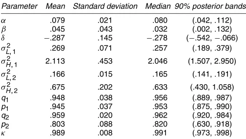
Table 2. Posterior Moments for the “Most Preferred” Model
Parameter Mean Standard deviation Median 90% posterior bands
α .079 .021 .080 (.042, .112)
NOTE: Results are for model IV with structural break assumption (B) and one structural break.
Comparing models III and IV shows “very strong evidence” in favor of volatility feedback in every case. The implied log Bayes factors range from 4.75 for model IV over model III un-der assumption (C) with two breaks for each model to 6.74 for model IV over model III under assumption (A) of no structural breaks.
Table 2 reports posterior moments for model IV under as-sumption (B) with one structural break in the volatility process. The results make it clear why this is the “most preferred” model. In particular, although there is considerable uncertainty regarding the magnitude of the marginal price of volatility β, there is little doubt that the volatility feedback as captured by the parameterδis an important aspect of stock return dynamics. In particular, the 90% posterior bands forδ (−.542,−.066)do not include 0. Meanwhile, the reduction in the level and persis-tence of high volatility episodes after the structural break (com-pare σH2,1 withσH2,2 andp1 withp2) explains the support for
structural break assumption (B).
The strong evidence for a negative volatility feedback ef-fect reflects the fact that volatility feedback is easier to iden-tify than the marginal impact of a change in volatility on a single-period expected return because volatility feedback sum-marizes the present value impact of volatility on all expected future returns. As evidence of this, we note that when we con-sider an alternative basis for rejection sampling that only re-stricts the marginal impact parameterβto be the opposite sign of the volatility feedback parameter δ(i.e.,β·δ≤0), we find
(A) No structural break 0 −886.12 −735.01 −734.75 −728.01
(B) Structural breaks in volatility process 1 −778.32 −732.31 −733.14 −727.27
2 −776.72 −736.09 −737.08 −731.82
3 −776.05
4 −778.96
(C) Structural breaks in all parameters 1 −779.00 −733.36 −733.38 −728.28
2 −777.84 −738.13 −738.60 −733.85
3 −777.91
4 −782.00
NOTE: For each model, additional breaks are considered until the last break is no longer preferred for either structural break assumption (B) or (C).
nearly identical results to when we restrict β to be nonnega-tive. The 90% posterior bands for β are(.002, .127), whereas the posterior bands forδare(−.540,−.068). However, the log marginal likelihood given this alternative restriction on the prior and posterior distributions is−727.63, which means that there is “very slight evidence” in favor of the nonnegativity con-straint. We also consider the effect of relaxing the sign restric-tions entirely. Again, the 90% posterior bands for the volatility feedback parameter(−.586,−.166)do not include 0. However, the posterior mean for the marginal price of risk parameter is negative(−.071)with 90% posterior bands of(−.224, .093). The log marginal likelihood is −727.12 for the unrestricted model versus−727.27 when the nonnegativity constraints are imposed. Thus, there is “very slight evidence” in favor of an unrestricted model according to marginal likelihood analysis. However, other considerations discussed at the end of this sec-tion when we present estimates of the equity premium lead us to impose the nonnegativity constraints as a strong prior.
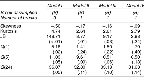
Given our results, a reasonable question is whether other models of stock returns would be preferable to model IV. For example, we could consider more complicated univariate mod-els that allow for a leverage effect and/or a third recurring volatility regime to capture the negative skewness and excess kurtosis of stock returns. Also, we could consider models with lagged returns or multivariate models to capture any apparent predictability in stock returns. However, Table 3 presents evi-dence suggesting that model IV captures many of the key fea-tures of stock return behavior with a relatively small number of parameters. First, we consider the sample skewness and kurto-sis of the standardized residuals for the preferred specifications of each model under consideration. Not surprisingly, model I, with its iid normal assumption, fails miserably at capturing the distribution of stock returns, even though two structural breaks in variance are allowed. Models II and III do a much better job capturing the excess kurtosis of the raw data, but they do not ap-pear to capture all of the negative skewness in returns. Model IV appears to explain most of the negative skewness and all of the excess kurtosis in the raw data. Second, we consider the mod-ified Ljung–Box Q-statistic tests of residual serial correlation. As discussed by Kim et al. (2001), a positive relationship be-tween the equity premium and the Markov-switching level of
Table 3. Diagnostics of Standardized Residuals for Preferred Model Specifications
Model I Model II Model III Model IV Break assumption (B) (B) (B) (B)
Number of breaks 3 1 1 1
Skewness −.50 −.17 −.16 −.09
Kurtosis 4.74 2.64 2.61 2.79
JB 148.71 8.77 9.17 2.88
(<.01) (.01) (.03) (.24)
Q(1) 5.18 1.41 1.50 .70
(.02) (.24) (.22) (.40)
Q(5) 11.03 9.61 10.51 8.50
(.05) (.09) (.06) (.13)
Q(24) 36.07 32.80 33.18 31.63
(.05) (.11) (.10) (.14)
NOTE: For each tests statistic, thep-value is reported in parentheses. JB stands for the Jarque-Bera test statistic for normality. Thep-value is based on a chi-squared(2) distribution under normality.Q(k) stands for the Ljung–Box test statistic for serial correlation at up toklags. Thep-value is based on a chi-squared(k) distribution under the absence of serial correlation.
market volatility implies a small degree of positive serial cor-relation in monthly returns. In particular, due to the persistence of the variance regimes, periods of above- (below-) average re-turns typically should be followed by more above- (below-) av-erage returns. The results of theQ-tests confirm that model IV does a reasonable job explaining the apparent short-horizon predictability in excess returns. Kim et al. (2001) showed that model IV can also explain the apparent long-horizon return pre-dictability (mean reversion in stock prices) reported by Fama and French (1988) and Poterba and Summers (1988). In light of these diagnostic test results, we argue that model IV is an ap-propriate model for conducting empirical analysis of structural changes in the distribution of stock returns.
Having established model IV as a reasonable empirical model of stock return behavior, we turn to the issue of struc-tural breaks. Returning to Table 1, there is support for as-sumption (B) of at least one structural break in the volatility process for every model. Comparing assumption (B) with as-sumption (A) of no structural breaks, the implied log Bayes factors range from .74 for model IV with one break to 110.07 for model I with three breaks. Also, comparing assumption (B) with assumption (C) of structural breaks in all parameters (except break probabilities), the implied log Bayes factors range from .24 for model III with one break to 2.04 for model II with two breaks. Comparing the “most preferred” model with model IV under assumption (C) with one break, the implied log Bayes factor is 1.01. However, note that because the equity pre-mium depends on the level of volatility for the “most preferred” model, the structural break in the volatility process still corre-sponds to a structural break in the equity premium. Meanwhile, there is “strong” or “very strong” evidence for only one break, except for model I. Comparing one break with two breaks for models II–IV, the implied log Bayes factors range from 3.78 for model II under assumption (B) to 5.57 for model IV under assumption (C). For model I, the evidence is strongest for three breaks. Comparing three breaks versus one break for model I under assumption (B), the implied log Bayes factor is 2.27. However, the support for multiple breaks for model I likely reflects the fact that, as with the model used by Pástor and Stambaugh (2001), the constant mean/constant variance speci-fication does not allow for transitory changes in volatility. Thus the model may be prone to confusing transitory but persistent changes in volatility with structural breaks.
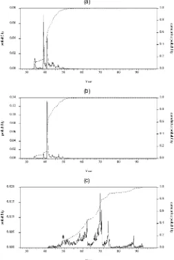
Just as important as the existence of a structural break in the equity premium is the timing and nature of the break. Figure 1 displays posterior distributions for the break dates for the “most preferred” model in panel (a) and for the preferred two-break model [model IV under assumption (B)] in panels (b) and (c). The posterior distributions in (a) and (b) suggest a break in the volatility process and, by implication, the equity premium sometime during the early 1940s. The corresponding cumula-tive distributions are very similar for the two models and are reasonably steep, implying a fair degree of certainty about the general timing of the structural break. In contrast, the cumu-lative distribution for the second break date for the preferred two-break model is reasonably flat, suggesting that the data are not particularly informative about a location for a second break date. Indeed, from the posterior distribution, the most proba-ble second break date has a<2% probability. Given this find-ing, it is not surprising that the marginal likelihood analysis
(a)
(b)
(c)
Figure 1. Posterior Distributions of Structural Breaks. The ity distribution (left scale) is the solid line and the cumulative probabil-ity distribution (right scale) is the dashed line. (a) The structural break in the “most preferred” model [model IV with structural break assump-tion (B) and one structural break]. (b) The first structural break in the preferred model given an assumption of two structural breaks [model IV with structural break assumption (B) and two structural breaks]. (c) The second structural break in the preferred model given an assumption of two structural breaks.
favors the one-break specification over the two-break specifi-cation for model IV. Comparing the “most preferred” model with the preferred two-break model, the implied log Bayes fac-tor is 4.55. Also, as an additional check for a second struc-tural break, we consider marginal likelihood analysis using the shorter sample period 1952–1999. The log marginal likeli-hood for model IV under assumption (A) of no structural break is−391.12, whereas the log marginal likelihood for model IV under assumption (B) with one structural break is −395.28. Thus the log Bayes factor in favor of no additional structural break in the postwar period is 4.16.
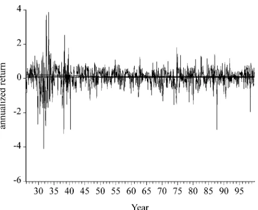
Figure 2 displays excess returns and estimates of the equity premium for the “most preferred” model. There is a clear re-duction in the general level and persistence of volatility during the 1940s, which is reflected in the reduction in the uncondi-tional equity premium and the persistence of the condiuncondi-tional equity premium over the same time period. Thus, as stocks
Figure 2. Excess Returns and the Equity Premium. Excess returns (left scale) are monthly value-weighted NYSE returns minus the yield on 1-month U.S. Treasury bills from CRSP. The measures of the equity premium (right scale) are from the “most preferred” model. The more volatile measure is the posterior mean of the equity premium conditional on the volatility regime. The smoother measure is the posterior mean of the unconditional equity premium.
became less risky after the structural break, the expected re-ward for investing in stocks declined as well. The reduced per-sistence of high-volatility episodes also suggests that volatility feedback may be less important in the postwar period, although the persistence of low-volatility regimes and the big negative returns in 1987 and 1998 suggest that it is still relevant. It is worth emphasizing, however, that the structural break in the equity premium appears to be driven entirely by the reduction in volatility (i.e., the “quantity of risk”), and not by a change in the risk preference parameters relating the equity premium to the level of volatility (i.e., the “price of risk”) or a change in volatility feedback. In particular, the marginal likelihood analysis favors constant risk preference parameters α and β
and the related volatility feedback parameterδacross structural regimes. This result suggests that the prebreak data contain rel-evant information about the postbreak behavior of stock returns and the equity premium.
Finally, with the most preferred model specification in hand and an understanding of the nature and timing of the structural break, we turn to the equity premium itself. As displayed in Figure 2, the posterior mean of the unconditional equity pre-miumµfor the “most preferred” model is about 12% near the beginning of the sample and drops to about 9% for most of the postwar period. The posterior mean of the conditional equity premium jumps between 10% and 16% in the volatile prebreak period. In the less volatile postwar period, the posterior mean of the conditional equity premium jumps between 9% and 10%. There is a large amount of uncertainty surrounding these point estimates, however. Figure 3 displays the posterior mean of the unconditional equity premium for the “most preferred” model along with 90% posterior bands. The 90% posterior bands are wide at the beginning of the sample and include the possibility that the equity premium is as high as 20%. After the structural break, the 90% posterior bands converge to 6% and 12%, which includes the sample mean of 6.5%. We also report 90% pos-terior bands for an unrestricted version of model IV under as-sumption (B) with one structural break that does not impose any
Figure 3. Uncertainty About the Equity Premium. The posterior mean and 90% posterior bands are for the “most preferred” model. The unre-stricted posterior bands are for model IV with assumption (B) and one break estimated without nonnegativity constraints. For computational tractability, the posterior bands are based on every tenth draw from the Gibbs sampler (i.e., 1,000 highly independent draws). [ posterior mean; 90% lower; 90% upper; 90% lower (unre-stricted); 90% upper (unrestricted).]
constraints on αandβ. The bands are much wider before the structural break and actually include negative values. We argue that this finding for the unrestricted model provides justification for our rejection sampling prior, because the rejection sampling produces results that are more in accordance with what we con-sider to be reasonable beliefs about the equity premium, namely that it is positive. However, we note that the rejection sampling has little impact on the 90% posterior bands after the structural break. Also, we note that the rejection sampling has no impact on the evidence in favor of a structural break in the volatility process. The log marginal likelihood for an unrestricted version of model IV under assumption (A) is−727.95, whereas the log marginal likelihood for an unrestricted version of model IV un-der assumption (B) with one break is−727.12. Therefore, the log Bayes factor in favor of a structural break of this form is .83, compared with .74 when the nonnegativity restrictions are im-posed. Thus we conclude from our analysis that the postwar unconditional equity premium is likely somewhere between 6% and 12%, with 9% as our point estimate.
An interesting question is why our point estimate is so much higher than the sample mean for excess returns and other esti-mates reported in recent studies (e.g., Fama and French 2002). In terms of the sample mean, we note that allowing for het-eroscedasticity in stock returns generally produces higher es-timates of the equity premium, because less weight is put on higher variance returns in estimation. It is well known that stock returns and market volatility are negatively correlated (see, e.g., French, Schwert, and Stambaugh 1987). As discussed by Kim et al. (2004), volatility feedback provides an explanation for this negative correlation given a positive underlying relation-ship between the equity premium and market volatility. Thus, by accounting for the volatility feedback effect, our model im-plicitly puts less weight on highly volatile returns associated
Figure 4. The Equity Premium in Perspective. Excess returns are monthly value-weighted NYSE returns minus the yield on 1-month U.S. Treasury bills from CRSP. The posterior mean of the unconditional equity premium and 90% posterior bands are for the “most preferred” model.
with changes in the volatility regime when estimating the eq-uity premium. In terms of our higher estimate than the values reported by Fama and French (2002), we note that if any of the decline in the dividend yield or increase in the price/earnings ratio over the past 50 years is permanent, then their point esti-mates of 2.5% and 4.3% understate the true equity premium.
A related concern is that the high estimated value for the eq-uity premium might somehow be implausible given other es-timates and theoretical considerations. We argue that, on the contrary, our estimate is quite plausible. First, we note that un-conditional sample standard deviation of excess returns is .653. Thus the classical 90% confidence bands for the equity pre-mium based on the sample mean and standard deviation cover the wide range of 3%–10%. Therefore, there is little sense from a purely econometric perspective that a point estimate of 9% is implausible just because the sample mean is around 6.5% and other estimates are lower. Another way to see this point is to notice that the scales in Figure 2 are vastly different. Fig-ure 4 plots excess returns, the posterior mean of the uncon-ditional equity premium, and the 90% posterior bands all on the same scale. From this perspective, the equity premium ap-pears essentially constant, and deciphering 6% from 12% is not particularly easy. Meanwhile, from a theoretical standpoint, the very possibility of structural change and the existence of transitory Markov-switching shifts in volatility could explain a high equity premium. As discussed by Wang (2001), shifts in volatility and the volatility process might generate a constant positive “jump-risk premium” making the unconditional equity premium higher than it would be given a stable iid normal dis-tribution.
6. CONCLUSIONS
We find evidence of a structural break in the equity pre-mium using data for excess returns on a value-weighted port-folio of NYSE stocks over the period 1926–1999. The break,
which likely occurred in the early 1940s, appears to be driven by a reduction in the general level and persistence of market volatility, not by a change in risk preferences. This finding sug-gests that although the overall distribution of excess returns has changed, there is still useful information about current behavior embedded in the prebreak data. The finding of a break in the eq-uity premium arises from a model of stock returns that relates the equity premium to the Markov-switching level of volatil-ity and allows for volatilvolatil-ity feedback in the event of unantici-pated changes in the volatility. The Bayesian model selection used in this article strongly favors this model over three more basic models of excess returns that either do not relate the eq-uity premium to changes in the level of volatility or do not ac-count for volatility feedback. Our analysis also suggests that our “most preferred” model captures most of the negative skewness, excess kurtosis, and short-horizon serial correlation in monthly stock returns. According to the model, the postbreak uncon-ditional equity premium is about 9%. Finally, there is strong evidence against a second structural break during the postwar period, including during the 1990s. In particular, the large cap-ital gains in the early and mid 1990s appear to be related to an unusually long period of low market volatility reminiscent of the 1950s and 1960s. Indeed, by the end of the sample in the late 1990s, it is clear that the extended period of low volatil-ity was only temporary, rather than the result of a permanent change in the volatility process.
ACKNOWLEDGMENTS
The authors have received helpful comments from Jeremy Piger, two anonymous referees, and participants in the CSSS seminar at the University of Washington and the “State-Space and Unobserved Components Models” academic colloquium in honour of James Durbin at the Royal Netherlands Academy of Arts and Sciences in Amsterdam. Responsibility for any er-rors is entirely their own. Support from the Ford and Louisa Van Voorhis Endowment at the University of Washington is gratefully acknowledged.
APPENDIX A: THE GIBBS SAMPLING APPROACH
To make inferences about model IV under assumption (C) with two structural breaks in all parameters, we need marginal posterior distributions for the following:
˜
In principle, the marginal posterior distribution of a set of para-meters can be obtained by integrating the other parapara-meters out of the joint posterior distribution
p(µ˜,σ˜2,D˜T,S˜T,S˜eT,p˜,κ˜| ˜YT).
However, the hierarchical nature of the model allows us to use Gibbs sampling to obtain the marginal posterior distributions of interest. This is done by successively sampling from the full conditional densities. The Gibbs sampling procedure involves the following steps:
independent of the other parameters.
4. Generateκ˜fromp(κ˜| ˜DT), where, conditional onD˜T,κ˜ is
independent of the other parameters.
5. Generateµ˜ fromp(µ˜| ˜σ2,D˜T,S˜T,S˜eT,Y˜T), where,
condi-tional onD˜T andS˜T,µ˜ is independent ofp˜ andκ˜.
6. Generateσ˜2 fromp(σ˜2| ˜µ,D˜T,S˜T,S˜eT,Y˜T), where,
con-ditional onD˜T andS˜T,σ˜2is independent ofp˜ andκ˜.
This procedure is a straightforward extension of Albert and Chib’s (1993) Bayes inference via Gibbs sampling for an au-toregressive time series subject to Markov-switching mean and variance. Kim and Nelson (1999b) extended the procedure to incorporate a one-time structural break in the Markov-switching parameters. Note that as a byproduct of generat-ing D˜T, we can get the marginal posterior distribution of the
break datesτ1andτ2.
The prior distributions are given as follows:
Parameters subject to structural breaks
αj∼N(0, .04)[α≥0], βj∼N(0, .04)[β≥0],
Here the subscript [·] function denotes a truncated distribu-tion obtained via rejecdistribu-tion sampling. Addidistribu-tional rejecdistribu-tion sam-pling occurs unless simulated structural regimes last at least 88 months, corresponding to 10% of the sample. All inferences are based on the last 10,000 of 12,000 Gibbs simulations (i.e., the first 2,000 simulations are discarded). Sensitivity analysis suggests that the qualitative results are robust with respect to a wide range of priors. We also examine convergence of the Gibbs sampler by trying different starting values for the para-meters and by comparing reported inferences to those from an additional 10,000 draws. We find that estimates are robust to the reported number of decimal places. We also note that the serial correlation of draws from the Gibbs sampler dies out monoton-ically, with simulated values more than 10 draws apart having less than 5% correlation.
APPENDIX B: CALCULATING THE MARGINAL LIKELIHOOD
Defineθ= { ˜µ′,σ˜2′,p˜′,κ˜′}′to be a vector of the model para-meters. Then, following Chib (1995), we can write the marginal density ofY˜t, by virtue of being the normalizing constant of the
posterior density, as
m(Y˜T)=
f(Y˜T|θ)π(θ)
π(θ| ˜YT)
,
where the numerator is the product of the sampling density and the prior, with all integrating constants included, and the de-nominator is the posterior density ofθ. Because the foregoing identity holds for anyθ, we may evaluatem(Y˜T)at the
poste-rior mean θ∗. Taking the logarithm of the foregoing equation for computational convenience, we have
lnm(Y˜T)=lnf(Y˜T|θ∗)+lnπ(θ∗)−lnπ(θ∗| ˜YT).
The log-likelihood function and the log of the prior density at θ =θ∗ can be evaluated relatively easily. First, the log-likelihood is given by
Second, the log of the prior density is given by
lnπ(θ∗)=lnπ(µ˜∗)+lnπ(σ˜2∗)+lnπ(p˜∗,κ˜∗),
where it is assumed that the parameter subsets are independent of each other.
For evaluating the posterior density at θ=θ∗, we consider the following decomposition of the posterior density:
π(θ∗| ˜YT)=π(µ˜∗| ˜YT)π(σ˜2∗| ˜µ∗,Y˜T)π(p˜∗,κ˜∗| ˜µ∗,σ˜2∗,Y˜T),
This decomposition of the posterior density suggests that
π(µ˜∗| ˜YT)can be calculated based on draws from the full Gibbs
run andπ(σ˜2∗| ˜µ∗,Y˜T)andπ(p˜,κ˜| ˜µ∗,σ˜2∗,Y˜T)can be
calcu-lated based on draws from reduced Gibbs runs,
ˆ
where the superscript “g” refers to the gth draw from the full Gibbs run and the superscript “gi,”i=2,3, refers to thegith
draw from the appropriate reduced Gibbs runs. Thus, apart from the usualGiterations for the full Gibbs run, we need additional 2×Giterations for the appropriate reduced Gibbs runs. For ex-ample, to calculateπ(p˜,κ˜| ˜µ∗,σ˜2∗,Y˜T), we need output from
an additionalGiterations for the following reduced Gibbs run: 1. Generatep˜andκ˜ fromp(p˜,κ˜| ˜µ∗,σ˜2∗,D˜T,S˜T,S˜eT,Y˜T).
Note that throughout the reduced Gibbs run,µ˜ andσ˜2are not generated, but are set equal to their posterior meansµ˜∗andσ˜2∗.
[Received November 2002. Revised June 2004.]
REFERENCES
Albert, J. H., and Chib, S. (1993), “Bayes Inference via Gibbs Sampling of Autoregressive Time Series Subject to Markov Mean and Variance Shifts,”
Journal of Business & Economic Statistics, 11, 1–15.
Carlin, B. P., and Chib, S. (1995), “Bayesian Model Choice via Markov Chain Monte Carlo Methods,”Journal of the Royal Statistical Society, 57, 473–484. Carlin, B. P., and Polson, N. G. (1991), “Inference for Nonconjugate Bayesian Models Using the Gibbs Sampler,” Canadian Journal of Statistics, 19, 399–405.
Chib, S. (1995), “Marginal Likelihood From the Gibbs Output,”Journal of the American Statistical Association, 90, 1313–1321.
(1998), “Estimation and Comparison of Multiple Change-Point Models,”Journal of Econometrics, 86, 221–241.
Fama, E. F., and French, K. R. (1988), “Permanent and Temporary Components of Stock Prices,”Journal of Political Economy, 96, 246–273.
(2002), “The Equity Premium,”Journal of Finance, 57, 637–659. French, K. R., Schwert, G. W., and Stambaugh, R. F. (1987), “Expected Stock
Returns and Volatility,”Journal of Financial Economics, 19, 3–29. Garcia, R. (1998), “Asymptotic Null Distribution of the Likelihood Ratio Test in
Markov Switching Models,”International Economic Review, 39, 763–788. George, E. I., and McCulloch, R. E. (1993), “Variable Selection via Gibbs
Sam-pling,”Journal of the American Statistical Association, 88, 881–889. Geweke, J. (1996), “Variable Selection and Model Comparison in Regression,”
inBayesian Statistics 5, eds. J. O. Berger, J. M. Bernardo, A. P. Dawid, and A. F. M. Smith, Oxford, U.K.: Oxford University Press, pp. 609–620. Hansen, B. E. (1992), “The Likelihood Ratio Test Under Nonstandard
Con-ditions: Testing the Markov-Switching Model of GNP,”Journal of Applied Econometrics, 7, S61–S82.
Jeffreys, H. (1961),Theory of Probability(3rd ed.), Oxford, U.K.: Clarendon Press.
Kass, R. E., and Raftery, A. E. (1995), “Bayes Factors,”Journal of the American Statistical Association, 90, 773–795.
Kim, C.-J., Morley, J. C., and Nelson, C. R. (2001), “Does an Intertempo-ral Trade-off Between Risk and Return Explain Mean Reversion in Stock Prices?”Journal of Empirical Finance, 8, 403–426.
(2004), “Is There a Positive Relationship Between Stock Market Volatility and the Equity Premium?”Journal of Money, Credit, and Bank-ing, 36, 336–360.
Kim, C.-J., and Nelson, C. R. (1999a),State-Space Models With Regime Switch-ing: Classical and Gibbs-Sampling Approaches With Applications, Cam-bridge, MA: MIT Press.
(1999b), “Has the U.S. Economy Become More Stable? A Bayesian Approach Based on a Markov-Switching Model of the Business Cycle,”
Review of Economics and Statistics, 81, 608–616.
(2001), “A Bayesian Approach to Testing for Markov Switching in Univariate and Dynamic Factor Models,”International Economic Review, 42, 989–1013.
Koop, G., and Potter, S. M. (1999), “Bayes Factors and Nonlinearity: Evidence From Economic Time Series,”Journal of Econometrics, 88, 251–281. Merton, R. C. (1980), “On Estimating the Expected Return on the Market:
An Exploratory Investigation,”Journal of Finance, 8, 323–361.
Pástor, L., and Stambaugh, R. F. (2001), “The Equity Premium and Structural Breaks,”Journal of Finance, 56, 1207–1239.
Poterba, J. M., and Summers, L. H. (1988), “Mean Reversion in Stock Prices: Evidence and Implications,”Journal of Financial Economics, 22, 27–59. Turner, C. M., Startz, R., and Nelson, C. R. (1989), “A Markov Model of
Het-eroskedasticity, Risk, and Learning in the Stock Market,”Journal of Finan-cial Economics, 25, 3–22.
Verdinelli, I., and Wasserman, L. (1995), “Computing Bayes Factors Using a Generalization of the Savage–Dickey Density Ratio,”Journal of the Amer-ican Statistical Association, 90, 614–618.
Wang, Z. (2001), Discussion of “The Equity Premium and Structural Breaks,” by L. Pástor and R. F. Stambaugh,Journal of Finance, 56, 1240–1246.