Full Terms & Conditions of access and use can be found at
http://www.tandfonline.com/action/journalInformation?journalCode=ubes20
Download by: [Universitas Maritim Raja Ali Haji] Date: 11 January 2016, At: 22:17
Journal of Business & Economic Statistics
ISSN: 0735-0015 (Print) 1537-2707 (Online) Journal homepage: http://www.tandfonline.com/loi/ubes20
Long-Run Identification in a Fractionally Integrated
System
Rolf Tschernig , Enzo Weber & Roland Weigand
To cite this article: Rolf Tschernig , Enzo Weber & Roland Weigand (2013) Long-Run
Identification in a Fractionally Integrated System, Journal of Business & Economic Statistics, 31:4, 438-450, DOI: 10.1080/07350015.2013.812517
To link to this article: http://dx.doi.org/10.1080/07350015.2013.812517
View supplementary material
Accepted author version posted online: 20 Jun 2013.
Submit your article to this journal
Article views: 200
Supplementary materials for this article are available online. Please go tohttp://tandfonline.com/r/JBES
Long-Run Identification in a Fractionally
Integrated System
Rolf T
SCHERNIGUniversity of Regensburg, Department of Economics, D-93040 Regensburg
Enzo W
EBERUniversity of Regensburg, Department of Economics, D-93040 Regensburg, Institute for Employment Research (IAB), D-90478 Nuremberg, and Institute for East and Southeast European Studies, D-93047 Regensburg
Roland W
EIGANDInstitute for Employment Research (IAB), D-90478 Nuremberg ([email protected])
We propose an extension of structural fractionally integrated vector autoregressive models that avoids certain undesirable effects on the impulse responses that occur if long-run identification restrictions are imposed. We derive the model’s Granger representation and investigate the effects of long-run restrictions. Simulations illustrate that enforcing integer integration orders can have severe consequences for impulse responses. In a system of U.S. real output and aggregate prices, the effects of structural shocks strongly depend on the specification of the integration orders. In the statistically preferred fractional model, shocks that are typically interpreted as demand disturbances have a very brief influence on GDP. Supplementary materials for this article are available online.
KEY WORDS: Fractional cointegration; Long memory; Misspecification; Structural VAR.
1. INTRODUCTION
The analysis of impulse responses to structural shocks pro-vides an indispensable tool for studying the dynamics of eco-nomic models. Shocks to dynamic systems are often classified with respect to their long-run effects. These shocks are referred to astransitoryif their impact eventually vanishes and otherwise are referred to aspermanent. Shocks with permanent effects can only occur in the presence of at least one variable integrated of order one or higher. Unlike other researchers in this area, we re-fer to a shock aspersistentif its impact is long-lasting, regardless of whether it is permanent or transitory.
To identify economically meaningful shocks using structural vector autoregressive (structural VAR) models requires identi-fication restrictions. Blanchard and Quah (1989) introduced the notion of constraining the long-run effect of a specific shock according to economic theory. For example, in the stylized ag-gregate supply/agag-gregate demand framework of Bayoumi and Eichengreen (1994), the permanent impact of demand innova-tions on GDP is constrained to zero, whereas prices may react permanently to both demand and supply shocks.
In this literature, GDP and prices are frequently modeled as variables integrated of order one (I(1)), where the impact of transitory shocks vanishes at an exponential rate. However, this does not guarantee that shocks will die out quickly, that is, within a few quarters. For example, based on a bivariate structural vec-tor auvec-toregressive model of post-war U.S. GDP and prices, the impulse responses of GDP to a demand shock remain substan-tial after 10 years (Section 4.4,Figure 3). If, however, prices are assumed to beI(2) instead ofI(1), Quah and Vahey (1995), the transitory shocks will die out within a few periods ( Fig-ure 4). Logically, appropriately specifying the integration order
is of crucial importance in impulse response estimation. The consequences of integer order misspecification have recently been addressed by Christiano, Eichenbaum, and Vigfusson (2003), Gospodinov (2010), and Gospodinov, Maynard, and Pesavento (2011).
Allowing for fractional orders of integration avoids the limi-tations of integer values. However, using a standard VAR model for fractionally differenced series (here GDP and prices) may still impose an undesirable restriction: if GDP is integrated of an order less than one, the responses of GDP to a long-run restricted shock must be negatively integrated. The appropriateness of this requirement is questionable given that the sum of the impulse responses over all periods is then zero. Another type of restric-tion occurs for the VARd,bmodel suggested by Johansen (2008). In its bivariate case the memory behavior of the restricted shock to GDP is determined by the difference between the integration orders of prices and GDP.
To avoid such problematic restrictions, we suggest a specific extension of the VARd,bmodels. Our structural fractionally inte-grated VARbmodel contains the standard fractional VAR model as a special case and can be restricted such that identification based on long-run zero constraints requires the restricted shock to only have a short-memory influence on GDP (as in classi-cal structural VAR models). Moreover, the unrestricted shock exhibits persistent effects due to long memory without being forced to have a permanent impact as in the traditional case.
© 2013American Statistical Association Journal of Business & Economic Statistics
October 2013, Vol. 31, No. 4 DOI:10.1080/07350015.2013.812517
438
Existing fractional models may suffer from severe misspecifi-cation bias with respect to impulse response estimation.
We show that extending our structural fractionally integrated VARb model through fractional cointegration is equivalent to generalizing the Johansen (2008) VARd,bmodel with respect to numerous differing fractional orders. From the Granger repre-sentation of our model, it follows that imposing the traditional long-run zero restriction (Blanchard and Quah 1989) implies that the rate of decay of the responses to the restricted shock is more rapid than in the case of the unrestricted shock.
Moreover, we propose a two-step estimator that corresponds to maximum likelihood estimation after the elimination of de-terministic trends. In simulations, we assess the performance of this method and find severe consequences of misspecified inte-ger integration orders for a stylized setting that is motivated by the empirical application of the method to GDP and prices in Section4.2.
Using our fractional model in the empirical investigation, we reject integer integration orders for GDP and price level. The long-run restricted shock has a small and relatively short-lived effect on real GDP compared to the unit root specification. This article is structured as follows. The next section presents our model and methods to identify the structural disturbances. Sec-tion3discusses the estimation and Section4contains empirical results for U.S. data. The last section concludes.
2. AN APPROPRIATE STRUCTURAL FRACTIONAL VAR WITH LONG-RUN RESTRICTIONS
In this section, we adopt the class of fractional vector time series models suggested by Johansen (2008) for structural anal-ysis. In this way, we provide a natural and useful means of cir-cumventing the limitations of standard integrated VAR models. Furthermore, we explain how the interpretation of the traditional long-run zero restriction (Blanchard and Quah1989) changes if the integration orders are noninteger values.
We assume a stochastic process with deterministic linear trends yt =ν0+ν1t+xt, where xt is generated by a very general reduced form linear time series model
Π(L)xt =ut, ut ∼IID(0;Ω), t =1,2, . . . . (1) HereΠ(L)=I+Π1L+Π2L2+ · · · is a potentially infinite order VAR polynomial that we specify below.
To obtain a solution for process (1) for a nonstation-ary xt, we apply the truncated operator notation (Johansen 2008, Appendices A.4, A.5) Π+(L)xt =1{t≥1}
t−1 i=0Πixt−i and Π−(L)xt =Π(L)xt−Π+(L)xt. Under mild conditions for the initial valuesxt,t ≤0, (see, e.g., Johansen and Nielsen 2012), the solution is given by
xt =Π+(L)−1ut+µt with µt = −Π+(L)−1Π−(L)xt, (2)
whereµtcaptures the impact of the initial values and where the coefficients of the inverse are determined by expandingΠ(z) around zero.
We refer to a univariate stationary linear processxt =φ(L)ut with square summable coefficients as an I(0) process if its spec-trum at frequency zero is continuous, bounded, and positive. Moreover, we will refer to the truncated versionφ+(L)ut, which
is a nonstationary but asymptotically stationary process, as I(0). For multivariate processes, we refer to univariate integration orders componentwise, and hence, no multivariate definition will be required.
For ease of presentation, we discuss models for bivariate time series, which are given by GDP and prices in the underlying ap-plication: yt=(gdpt pt)′. Thek-dimensional case is discussed at the end of Section2.2and in AppendixA.
We employ a structural VAR withut =Bεt to identify eco-nomically meaningful shocks. Here Bis the impact matrix that contains the contemporaneous effects of structural shocksεt = (ε1,t ε2,t)′ on the economic variables xt =(x1,t x2,t)′. Identi-fication assumptions are required to obtain the four unknown coefficients of B. After normalizing var(εt)=I, which yields three distinct equations in B B′=Ω, one further restriction is demanded to fully determine B.
Toward this end, we will constrain the influence ofε2,t on x1,t+hfor large horizonshin the spirit of Blanchard and Quah (1989). We, therefore, labelε2,t the long-run restricted shock (LRRS), although its effect on x2,t+h is unrestricted. In con-trast, we refer toε1,t as the long-run unrestricted shock (LRUS). In a basic AD/AS model, LRUS and LRRS can be straight-forwardly interpreted as aggregate supply and demand shocks, respectively. Alternatively, based on Phillips curve considera-tions, LRUS and LRRS have been treated as shocks to core inflation (LRRS) and noncore inflation (LRUS); see Quah and Vahey (1995).
2.1 Limitations of Available Structural Fractionally Integrated VAR Models
In an integrated VAR setting in which both elements ofxtare integrated of order one but are not cointegrated, (1) holds with
Π(L)=A(L)=(I−A1z− · · · − Apzp)(1−L) and all so-lutions of|A(z)| =0 outside the unit circle. Thus, the first dif-ferences of the series follow a stable finite-order VAR. We call this model an IVAR(1,1) model or, more generally, IVAR(d1,d2) if the differences in integer ordersd1andd2renderd1x1,t and d2x
2,t integrated of order zero.
Based on the well-known Granger representation theorem, the IVAR(1,1) model can be stated as
xt =Ξ(1) (LRR), which implies that the LRRS has no permanent effect on the first variable, corresponds to
Ξ(1)=A(1)−1B=
Ifd1andd2are allowed to be real-valued, the standard mod-eling approach considers fractionally integrated VAR (FIVAR) models; see, for example, Nielsen (2004). Then, fractional dif-ferences rather than first difdif-ferences of the variables are modeled as a stable vector autoregression such thatΠ(L)= A(L)∆(L;d)
with∆(L;d1, d2)=diag(d1, d2). The fractional differencing operatordis given by a power expansion as follows:
d =(1−L)d =π
0+π1L+π2L2+ · · · with πj =
Ŵ(j −d)
Ŵ(−d)Ŵ(j+1), (5) whereŴ(.) denotes the Gamma function.
Technically, restriction LRR (4) can be imposed in precisely the same manner as in the IVAR(1,1) case, because onlyA(.) and
Ωare required to computeB. To clarify the implications of LRR (4) in the FIVAR model, we consider its Granger representation
xt = which follows from the general specification (A.3) derived in AppendixAforb=1. Imposing LRR (4) in this case allows us to write the first variable as
x1,t =
LRUS: persistent and short-lasting component
+ 1−d1
+ ξ+∗,12(L)ε2,t+μ1,t
LRRS: short-lasting component .
The impulse responses with respect to the structural shocks are given by the coefficient matricesΘh of the MA represen-tationxt =Θ+(L)εt+µt. Theskth elementθsk,h denotes the impulse response of thesth variable to thekth shock at horizon h. By the first term in (6), the impulse responses ofx1to the unre-stricted shock evolve according toθ11,h=O(hd1−1). They decay slowly if the GDP is nonstationary and 0.5< d1 <1, whereas they converge to a constant in the unit root case (d1=1) and diverge ford1>1.
In contrast, when imposing LRR (4), we see that by the sec-ond term in (6), the responses to the restricted shockθ12,hare at mostO(hd1−2) and hence converge to zero even if 1< d
1<2. In the case in which ξ12∗(1)=0, the order is even lower; see the discussion of (A.4) in Appendix A. If d1<1, as recent evidence suggests for real GDP, the short-lasting component 1−d1
+ ξ+∗,12(L)ε2,thas a negative integration order ofd1−1<0. One implication of this finding is that the impulse responses of the identified LRRS sum to zero, exhibiting at least one sign change. This is unreasonably restrictive if the LRRS is inter-preted as, for example, shocks to aggregate demand. Moreover, the impulse response function approaches zero at the slow hy-perbolic ratehd1−2. In sum, imposing LRR (4) in FIVAR models
leads to unsatisfactory and overly restrictive properties of the identified LRRS. The VARd,bprocess as proposed by Johansen (2008) is an alternative specification for modeling multivariate fractional integration. It suffers from a comparable restriction as is explained at the end of the next section.
2.2 Structural Fractionally Integrated VARbModels
As a solution to these problems, we propose a model for short-run dynamics that is related to Johansen’s (2008) approach and
that generalizes standard (F)IVAR models. First, we callηt a VARbprocess if it follows
A(Lb)ηt =ut, (7)
whereA(z) is a matrix polynomial of orderpas before. However, (7) extends the standard finite-order VAR because of the use of the fractional lag operatorLb :=1−b. By construction,Lbηt is a weighted sum of pastηt, which supports the notion ofLb as a lag operator. Forb=1, we haveL1=Landηt follows a standard vector autoregression. Ifzt isI(d), thenLbzt retains this property because it can be written as the sum of anI(d) and anI(d−b) variable, where the larger order dominates.
We impose the stability condition (Johansen2008, Corollary 6) onA(·) andbunder which each component ofηt generated by (7) is anI(0) process. The stability of theA(Lb) polynomial also implies thatA(1) is nonsingular. Under this condition, the parameterbadds some flexibility to theshort-runproperties of the process rather than influencing the integration orders.
By insertingηt =(L;d)xt into (7), we obtain and propose the fractionally integrated VARb(FIVARb) model
A(Lb)(L;d)xt =ut, t=1,2, . . . . (8) For the FIVARbmodel, the Granger representation is given by
xt = a special case of itsk-variate version (A.3) derived in Appendix
A. Under LRR (4), the LRUS and LRRS components driving the first variable are
LRUS: persistent and short-lasting component
+ b−d1
such that the short-lasting component ofx1,t is in general in-tegrated of orderd1−b. In the discussion following Equation (A.3) in AppendixA, we address a case in which the integration order of the restricted component is reduced even further (to d1−2b).
Thus, in the FIVARb model, the parameterb influences the memory property of the short-lasting component in general through b−d1
+ (or through 2b−d1
+ ) and thus offers additional flexibility compared to the FIVAR specification and the standard VARd,b model (11) presented below. Given condition (A.4) in AppendixA, fluctuations inx1,t due to the LRRS exhibit long memory behavior if 0< b < d1, negative integration ifb > d1 and short memory only ifb=d1. This short memory restriction can be tested against the data. Note that a necessary condition for the stationarity of this short-lasting component isd1−b <0.5. The IVAR(1,1) model is a special case in which the LRRS can only imply short memory effects.
Above, we mentioned that the standard VARd,b model of Johansen (2008) does not provide sufficient flexibility for struc-tural analysis. To allow for different integration orders, consider
a VARd,b model with the fractional cointegration relationship It has solution (Johansen2008, Theorem 8)
xt =−+dC ut+b+−dC ∗u
t+2+b−dH+(Lb)ut+µt, (12) where the special structure ofβ=(1 0)′implies that the first row ofC contains only zeros, as seen from the general expression forCin AppendixA. As noted by one of the reviewers, setting d =d2,b=d2−d1>0 andut= Bεtyields cannot be imposed on the first term on the right-hand side; rather, it has to be imposed onC∗B instead. Model (11) is a FIVARbwith the restrictionb=d2−d1; for verification, insert d2Lj
(11) and rearrange the terms. Therefore, the impact of the LRRS onx1,t in (11) in general has integration orderd−2b=2d1− d2. It is only in the special case of 2d1=d2in which the impact of LRRS is short-memory.
FIVARbmodel (8) can be extended to ak-dimensional series xt if ∆(L;d) :=diag(d1, . . . , dk). We emphasize that the k-dimensional FIVARb model and the VARd,b model can be generalized such that both are included as special cases, which will yield the fractionally cointegrated VARbmodel (FCIVARb)
∆(L;d)xt =αβ′Lb∆(L;d−b)xt which is obtained from (8) by adding the error correction term αβ′L
b∆(L;d−b)xt. Alternatively, (14) can be stated as an extended VARd,b model (VARd1,...,dk,b model) if ˜xt :=
∆(L;d−b)xt for which the Johansen (2008) VARd,b model withd =bholds. Here, the (k×k) matrices Aj play the role of Johansen’sΓj. The solution to (14) and further discussion are included in AppendixA. An example of model (14) was recently presented by Søren Johansen in a research seminar. To assess the validity of the baseline FIVARb model against the more general specification (14) in the bivariate case, we suggest to use nonparametric cointegration tests for the null of no frac-tional cointegration of (d1−bx
1t, d2−bx2t)′or equivalently of (x1t, d2−d1x2t)′ifd2> d1; see Section4.1.
3. ESTIMATION AND SPECIFICATION
3.1 Estimation of FIVARbModels With Deterministic Trends
Under the assumption of fixed, potentially nonzero but bounded initial values, asymptotic properties of maximum like-lihood estimators are available for models that are related to
the FIVARbmodel (Nielsen2004; Johansen and Nielsen2012). Due to the similarity of these models, we expect the maximum likelihood estimators ofd,b, andAjin our model to also exhibit standard asymptotic properties. AppendixBdemonstrates that the parameters of the bivariate FIVARbmodel are identified if
Ap =Oand if the A(Lb) polynomial is stable.
Leaving aside deterministic terms, the Gaussian log-likelihood of the FIVARbmodel is
L(d, b,α,Ω)= −n timization problem can be reduced to a three-dimensional prob-lem ind1,d2, andbby concentrating the log-likelihood function. The estimate ofαis obtained via least squares from a regression of∆(L;d)xton∆(L;d)Lbxt,. . .,∆(L;d)L
p
bxt;Ωis estimated from the corresponding residuals.
As in Section 2, we allow for deterministic terms, that is, nonzero means and linear time trends, which we account for in a two-step estimation procedure. Tschernig, Weber, and Weigand (2013) find that estimating the deterministic terms in the like-lihood optimization may lead to poor results in finite samples. The authors provide simulation evidence and a line of reasoning that explains why the estimator defined using the two following steps is more robust.
In the first step, the integration ordersds,s=1,2 are esti-mated using the semiparametric exact local Whittle estimator of Shimotsu (2010), which allows for deterministic trends. Based on ˆds, the parametersν0andν1in are estimated using least squares. In the second step, the log-likelihood (15) is maximized for the trend-adjusted series ˆxt =
yt−νˆ0−νˆ1t.
3.2 A Small Monte Carlo Study
The following simulation will illustrate the behavior of the two-step procedure described in Section 3.1and various likelihood-ratio tests based upon it that are used in Section4.2. We present the results for two data-generating processes, each with one lag:
FIVARb1.This specification matches integration orders, the reduced form error covariance matrix and the A(1) matrix of a FIVARd1model with four lags fitted to GDP and prices
in Section4.2such that the impact matrix Band the long-run characteristics given by the first term in the Granger representation (9) are identical:
IVAR1. This specification matches the reduced form error covariance matrix and the A(1) matrix of an IVAR(1,1) model with four lags fitted to GDP and prices in Section
4.2:
1 0 0 1
−
0.26 −0.24 0.12 0.96
L 0
0
xt =ut,
Ω =
7.4 −0.2
−0.2 0.77
. (18)
For both (17) and (18), 5000 processes of length 250 are sim-ulated with Gaussian innovations from which 28 observations are used as presample values. This choice corresponds to the empirical application in Section4. Deterministic terms are not included in the generating processes because the estimated im-pulse responses are invariant with respect to them. The param-eters are estimated by assuming an IVAR(1,1), IVAR(1,2) or FIVARd1 model with the correct lag length and LRR (4)
im-posed. The FIVARd1 specification is estimated using the
two-step procedure described above with 15 frequencies for the semi-parametric memory estimator in the first step. The concentrated log-likelihood is maximized by conducting a grid search and applying a nonlinear maximization routine.
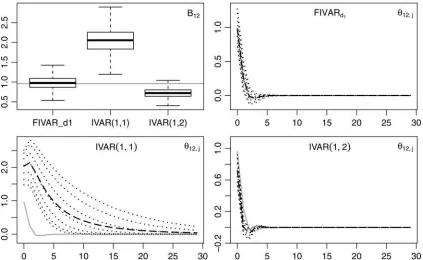
Figures 1and2present boxplots of the estimated impact co-efficientsb12 in the upper left graphs. All other graphs display the true impulse responses (represented by the gray solid line) of the data-generating mechanism along with the means of the es-timates (represented by the dashed line) and the 5%, 10%, 25%, 50%, 75%, 90%, and 95% quantiles (represented by the dotted lines) for the different models. Because of space limitations, we restrict our attention to the responses of the first variable to
LRRS. The estimates from the FIVARd1model provide reliable
inferences for process (17), with estimates centered at the true values as shown inFigure 1. The estimated IVAR(1,1) impulse responses are misleading due to their slow convergence to zero. The observed slow convergence mirrors asymptotic results and additional simulation results for a simple stylized setup that are provided in the supplementary material. Interestingly, the sam-pling uncertainty is greater than in the fractional model even though the integration orders are fixed rather than estimated. The IVAR(1,2) model understates the impact coefficient and im-pulse responses, which follows from discarding zero-frequency information by over-differencing.
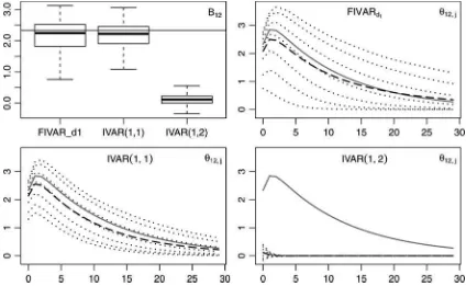
To assess the efficiency loss from using a fractional model when the unit root assumption holds, we estimate all three spec-ifications for the IVAR1 process (18). As can be observed from
Figure 2, the increase in variance is noticeable but is rather small relative to the strong misspecification effects shown in the lower left panel ofFigure 1, which can be avoided.
Next, using our two-step procedure, we analyze the proper-ties of the hypothesis tests applied in Section4.3for bin the fractional lag operator and, imposingb=d1as a familiar restric-tion, for the integration ordersd1andd2. For 10,000 iterations, likelihood-ratio test statistics are computed from the likelihoods of the trend-adjusted series and are employed to test different hypotheses using critical values from theχ2-distribution. The results for the fractional data-generating process (17), which are shown inTable 1, exhibit good size properties (see the first four lines of the table) and excellent power, at least for the hypothe-ses concerningd1andd2 (see the lower lines). The low power against b=1 is due to the proximity of the null to the true value; here, the short-memory dynamics associated withb com-pete with the flexibility introduced through the VAR coefficients.
Figure 1. Upper left: Boxplots of estimated impact coefficients. All other: Mean (dashed) and quantiles (dotted) of estimated impulse responses of the first variable to LRRS according to a FIVARd1, IVAR(1,1), and IVAR(1,2) specification. The gray solid lines correspond to the
true impact coefficients and impulse responses of the FIVARb1 process (17) of which 5000 replications with 250 observations were drawn.
Figure 2. Upper left: Boxplots of estimated impact coefficients. All other: Mean (dashed) and quantiles (dotted) of estimated impulse responses of the first variable to LRRS according to a FIVARd1, IVAR(1,1), and IVAR(1,2) specification. The gray solid lines correspond to the
true impact coefficients and impulse responses of the IVAR1 process (18) of which 5000 replications with 250 observations were drawn.
The size is also reasonable for the I(1) data-generating process (18) inTable 2. The over-rejection of true hypotheses for the smaller sample size (n=250) may be due to a relatively strong persistence in the VAR polynomial and is reduced in larger sam-ples (n=1000). Again, the tests are very powerful against the hypotheses that we consider in the lower part of the table.
Additional Monte Carlo results are provided in the electronic supplement. We find that the outcomes become less simple if processes and specifications with more lags are considered. Higher VAR orders increase the variance of the estimated im-pulse responses, and underspecifying the order in a FIVARb model may lead to severe underestimation of the responses of the first variable to LRRS. Moreover, we show for a very stylized
data-generating process that neither the VARd,bmodel (11) nor the FIVAR model provides sufficient flexibility to adequately model the dynamic effects of LRRS. Severe misspecification effects are found for both the short and long horizons.
4. STRUCTURAL ANALYSIS OF GDP AND PRICES
In this section, our structural fractionally integrated VARb model (8) is fitted to output and price data using the two-step procedure outlined in Section 3.1and is tested against nested integer and fractional alternatives. We employ quarterly time series for the natural logarithms of the U.S. real gross domestic
Table 1. Rejection frequencies of hypotheses aboutd1,d2, andbfor the FIVARb1 process
n=250 n=500 n=1000
H0 Nom. level 0.01 0.05 0.1 0.01 0.05 0.1 0.01 0.05 0.1
b=0.83 0.022 0.085 0.147 0.015 0.065 0.124 0.014 0.058 0.112
d1=0.83,d2=1.77 0.017 0.071 0.130 0.012 0.060 0.113 0.011 0.053 0.107
d1=0.83 0.013 0.061 0.118 0.011 0.054 0.105 0.011 0.055 0.105
d2=1.77 0.016 0.065 0.121 0.013 0.057 0.110 0.011 0.054 0.102
b=0.5 0.253 0.481 0.608 0.466 0.701 0.799 0.790 0.925 0.958
b=1 0.021 0.085 0.150 0.067 0.191 0.286 0.211 0.425 0.549
b=1.5 0.832 0.935 0.965 0.998 1.000 1.000 1.000 1.000 1.000
d1=1,d2=1 0.999 1.000 1.000 1.000 1.000 1.000 1.000 1.000 1.000
d1=1,d2=2 0.894 0.974 0.989 0.999 1.000 1.000 1.000 1.000 1.000
d1=1 0.564 0.792 0.869 0.925 0.981 0.992 0.999 1.000 1.000
d2=2 0.657 0.869 0.931 0.969 0.996 0.998 1.000 1.000 1.000
NOTE: The table gives rejection frequencies for eachH0over 10,000 realizations of the process (17). LR-tests are conducted with critical values from theχ2-distribution. For all tests
aboutd1andd2, we imposeb=d1under bothH0and the alternative hypotheses.
Table 2. Rejection frequencies of hypotheses aboutd1,d2, andbfor the IVAR1 process
n=250 n=500 n=1000
H0 Nom. level 0.01 0.05 0.1 0.01 0.05 0.1 0.01 0.05 0.1
b=1 0.030 0.103 0.171 0.031 0.105 0.175 0.030 0.099 0.165
d1=1,d2=1 0.026 0.094 0.156 0.019 0.071 0.131 0.013 0.061 0.114
d1=1 0.033 0.106 0.179 0.022 0.083 0.144 0.017 0.068 0.124
d2=1 0.021 0.076 0.141 0.016 0.064 0.122 0.012 0.055 0.108
b=0.5 0.526 0.749 0.836 0.840 0.945 0.972 0.994 0.999 1.000
b=1.5 0.644 0.821 0.881 0.963 0.991 0.996 1.000 1.000 1.000
d1=1,d2=1.5 0.740 0.880 0.924 0.974 0.989 0.994 1.000 1.000 1.000
d1=0.5,d2=1 1.000 1.000 1.000 1.000 1.000 1.000 1.000 1.000 1.000
d1=0.5 0.999 1.000 1.000 1.000 1.000 1.000 1.000 1.000 1.000
d2=1.5 0.650 0.828 0.887 0.965 0.987 0.991 1.000 1.000 1.000
NOTE: The table gives rejection frequencies for eachH0over 10,000 realizations of the process (18). LR-tests are conducted with critical values from theχ2-distribution. For all tests
aboutd1andd2, we imposeb=d1under bothH0and the alternative hypotheses.
product and its implicit price deflator, downloaded from Federal Reserve Economic Data (FRED) and ranging from 1947Q1 to 2009Q2.
4.1 Semiparametric Analysis
In the first step, the memory parameters are estimated us-ing the semiparametric exact local Whittle method (Shimotsu
2010) with different numbers of Fourier frequencies. We find real GDP to be integrated of order less than one, which con-firms the results reported in the literature (e.g., Diebold and Rudebusch1989; Caporale and Gil-Alana2013). The estimated integration orders for the price level are found to be between 1.5 and 1.8. This finding mirrors the coexistence of strategies that involve modeling inflation asI(1) orI(0) throughout the empirical literature. Based on 15 Fourier frequencies, we obtain
ˆ
d1=0.77 and ˆd2 =1.54. These estimates are used in (16) to estimate and eliminate the deterministic trends.
The FIVARb model (8) is not appropriate if the series are fractionally cointegrated. In such a case, the more general FCI-VARb model (14) introduced in Section 2.2 should be ap-plied, as this model allows for a cointegration rank of r =1 for ˜xt=(x1,t d2−d1x2,t). We apply the nonparametric test of Nielsen (2010) to the balanced series ˜xt, in which the dj’s are replaced by their semiparametric estimates. Usingztto de-note the least-squares trend-adjusted ˜xt, for a prespecifiedγ, we compute ˜zt =−+γzt, and then obtain Rn=nt=1ztz′tand Sn=nt=1˜zt˜zt′. The eigenvaluesλ1≤λ2ofR−n1Snare used to construct the test statisticr =n2γj2−=r1λj. To testH0:r =0 in our empirical application, we useγ =0.1 as suggested by Nielsen (2010). With a test statistic of0=3.5025, we fail to reject H0 at the 10% level and employ the FIVARb model in what follows.
4.2 Parameter Estimates
In the second step, we conduct a maximum likelihood es-timation based on the trend-adjusted ˆxt. For each VAR order p=0, . . . ,6, we consider various specifications for b, both without restrictions and under the constraintsb=1 (FIVAR), b=d1(FIVARbwith LRRS exhibiting a short-memory impact
on the first variable) and b=d2−d1 (a special VARd2,d2−d1
model). As in the simulation, 28 initial values (from 1947Q1 to 1953Q4) are used to compute fractional differences appearing in the likelihood (15). The concentrated log-likelihood is maxi-mized for starting values taken from a grid search overd1,d2and b. Because the parameters of the FIVARbmodel are only iden-tified ifA(Lb) is stable and Ap =O, we discard estimates that imply a nonstable polynomial and select the global maximum from the remaining local optima.
Table 3presents the log-likelihood, the AIC, and SC infor-mation criteria and the estimated integration ordersd1,d2, and bfor each model specification. Choosing lag orderpusing the information criteria, we find p=1 for the SC criterion and p=4 for the AIC criterion, regardless of the specification ofb. To provide sufficient flexibility to model dynamic interactions and given the quarterly sampling frequency, we preferp=4. For bothp=1 andp=4, the estimated integration orders are between 0.4 and 0.9 for GDP and between 1.6 and 1.9 for prices. For some of the other lag orders, we find roots of|A(·)|, which are close to the nonstable region. Because the VAR polynomial is then expected to capture a substantial amount of persistence, the integration orders may be severely underestimated. An ex-treme case is observed forp=5 with freely estimatedb and
ˆ d1≈0.
4.3 Tests onband Nonfractionality Hypotheses
We determine whether the flexibility of the FIVARb model is empirically necessary by conducting likelihood-ratio tests of various nested specifications. The Monte Carlo results in Sec-tion3.2indicate reasonable size and power properties for the cases investigated below. First, we are interested in whether the data significantly reject the standard fractionally integrated VAR model (b=1), whether b=d1 holds, and whether the Johansen (2008) restriction (b=d2−d1) can be maintained. Once we allow for sufficiently rich short-run dynamics through a reasonably large VAR orderp, it becomes difficult for us to statistically distinguish between different values of the parame-terb. Forp=4, which will be the model we employ hereafter, we do not reject any of the three hypotheses at conventional significance levels.
Table 3. Two-step estimation results of the FIVARbmodel (8) for quarterly postwar U.S. GDP and prices with different specifications forband lag lengthp
p LogLik AIC SC d1 d2 b
bnot incl. 0 304.38 −2.7242 −2.6935 1.3036 1.5950 —
bfree 1 319.09 −2.8116 −2.7043 0.4679 1.7497 0.9486
2 325.50 −2.8333 −2.6647 1.1050 1.8598 0.0000
3 330.25 −2.8401 −2.6102 1.1886 2.1575 0.2260
4 335.61 −2.8524 −2.5611 0.7230 1.7538 0.8983
5 338.66 −2.8438 −2.4912 0.0000 2.0663 0.4579
6 341.70 −2.8351 −2.4213 0.7807 1.8201 0.7435
b=1 1 318.98 −2.8196 −2.7276 0.4429 1.7408 1.0000
2 321.16 −2.8032 −2.6499 0.4922 0.7457 1.0000
3 327.21 −2.8217 −2.6071 0.5896 1.9866 1.0000
4 335.29 −2.8585 −2.5826 0.6600 1.7521 1.0000
5 336.24 −2.8310 −2.4938 0.7224 0.9085 1.0000
6 340.41 −2.8325 −2.4340 0.5894 1.7034 1.0000
b=d1 1 316.80 −2.8000 −2.7080 0.6827 1.8228 0.6827
2 324.10 −2.8297 −2.6765 0.5908 1.2157 0.5908
3 328.77 −2.8358 −2.6212 0.6832 1.8623 0.6832
4 335.39 −2.8594 −2.5835 0.8263 1.7714 0.8263
5 338.27 −2.8492 −2.5120 0.3615 2.2495 0.3615
6 341.69 −2.8441 −2.4456 0.7595 1.8037 0.7595
b=d2−d1 1 315.67 −2.7898 −2.6978 0.5831 1.6918 1.1087
2 324.26 −2.8312 −2.6779 0.6605 1.2192 0.5587
3 329.14 −2.8391 −2.6246 0.8957 1.4902 0.5946
4 335.49 −2.8603 −2.5844 0.7643 1.6748 0.9104
5 336.97 −2.8375 −2.5003 0.6718 1.3971 0.7253
6 341.06 −2.8383 −2.4398 0.7801 1.5888 0.8087
NOTE: For each specification ofbthe minimum of AIC and SC are in boldface.
The unit root behavior of GDP and price level was assumed in prior studies. With fractional alternatives, we find clear evi-dence againstH0:d1=d2=1 for most lag lengthsp. Forp=1 and our preferred specificationp=4, we reject this hypothesis at conventional significance levels; seeTable 4. A widespread alternative specification with a unit root inflation process, the IVAR(1,2) model corresponding toH0:d1=1 andd2=2, is also rejected at the 5% level given our baseline specification. Conducting the tests of nonfractional values ford1 andd2 in-dividually, we confirm the previous evidence that d1 =1 and d2 =1, whereas we cannot reject theI(2) hypothesis for prices forp >1. In summary, we find that the IVAR(1,1) model, which
Table 4. Tests of nonfractional hypotheses aboutd1andd2
H0 p bfree b=1 b=d1 b=d2−d1 d1=d2=1, 1 52.12∗∗∗ 52.12∗∗∗ 47.77∗∗∗ —
4 16.75∗∗∗ 16.75∗∗∗ 16.95∗∗∗ —
d1=1,d2=2 1 13.98∗∗∗ 22.31∗∗∗ 17.96∗∗∗ 15.69∗∗∗
4 3.31 8.57∗∗ 8.77∗∗ 8.98∗∗
d1=1 1 12.81∗∗∗ 23.53∗∗∗ 19.18∗∗∗ 6.43∗∗
4 2.07 3.84∗∗ 4.04∗∗ 1.87
d2=1 1 15.51∗∗∗ 48.37∗∗∗ 11.32∗∗∗ 22.01∗∗∗ 4 9.16∗∗∗ 6.71∗∗∗ 9.27∗∗∗ 10.28∗∗∗
d2=2 1 10.16∗∗∗ 13.20∗∗∗ 5.69∗∗ 15.58∗∗∗
4 2.24 2.87∗ 1.79 7.84∗∗∗
NOTE: The table gives likelihood-ratio test statistics. The stars indicate significance levels at whichH0is rejected using aχ2-distribution:∗10%,∗∗5%,∗∗∗1%.
is the workhorse in the related literature, is misspecified. This finding also holds if prices are instead assumed to beI(2). Our fractional specification seems suitable for such situations.
4.4 Responses to Structural Shocks
The structural analysis in this section is performed by impos-ing the long-run zero constraint LRR (4) to identify shocks with short-lasting effect on output, LRRS, and shocks with a persis-tent effect, LRUS. Given the results presented in the previous sections, we can set the lag length to p=4 and impose the restrictionb=d1in the FIVARb model. Because ˆd2 ≈2 ˆd1for this specification, applying the VARd,bmodel (11) withd =d2 and b=d2−d1 yields similar results. As reference models, we consider an IVAR(1,1) and an IVAR(1,2) specification, each with four lags.
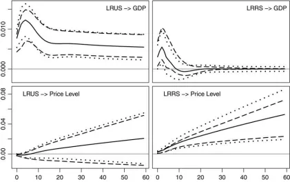
The estimated impulse responses of output and prices to the structural disturbances, given by the coefficients ˆθsk,h, are plot-ted against horizonhin the four panels ofFigures 3,4, and5. Bootstrapped 90% confidence intervals are simulated using the standard error method (dotted lines) and the percentile method (dashed lines), which are both discussed in Christiano, Eichen-baum, and Vigfusson (2007). We observe that moving from the IVAR(1,1) to the IVAR(1,2) model drastically alters the role of the shocks in both GDP and price development. The fractional setting indicates an intermediate scenario that is relatively sim-ilar to the specification with prices modeled as I(2).
Figure 3. Estimated impulse responses of an IVAR(1,1) model withp=4. Dotted lines are 90% confidence intervals based on bootstrap standard errors, dashed lines are bootstrap percentile confidence intervals.
Responses of output. First consider the effects of structural shocks on GDP. In the IVAR(1,1) model (see the upper panel of
Figure 3), responses to LRUS converge to a positive constant, the long-run effectξ11(1). The LRRS has significant effects for in-termediate horizons. The effects reach their maximum after two
quarters and then decay slowly. Even after 20 quarters, approx-imately half of the maximum impact remains. Both impulse re-sponse functions of GDP are very similar to those estimated in a bivariate output-unemployment system by Blanchard and Quah (1989). If LRRS is associated with a demand shock, the observed
Figure 4. Estimated impulse responses of an IVAR(1,2) model withp=4. Dotted lines are 90% confidence intervals based on bootstrap standard errors, dashed lines are bootstrap percentile confidence intervals.
Figure 5. Estimated impulse responses of a FIVARd1 model withp=4. Dotted lines are 90% confidence intervals based on bootstrap
standard errors, dashed lines are bootstrap percentile confidence intervals.
medium-run real effects will have far-reaching consequences for the understanding of business cycles and policy making.
These results contrast sharply with the results for the IVAR(1,2) specification; see the upper panel in Figure 4. Whereas the long-run effect of LRUS is of approximately the same magnitude, the estimated effects of LRRS are negligible even for short horizons. We consider the FIVARd1 model to
avoid an a priori decision between two specifications with fun-damentally different implications. The upper panel inFigure 5
presents the corresponding impulse responses. As GDP is esti-mated to be integrated of an order less than one, both structural shocks are transitory, and hence, the impulse responses eventu-ally decrease for both LRUS and LRRS. Although the decay of responses to LRUS is very slow, the effect of LRRS on output is small and short-lived unlike that obtained from the IVAR(1,1) model. This finding is consistent with the simulation evidence for misspecified IVAR processes that is reported in Section3.2. The responses are only significant for a short interval of hori-zons and become insignificantly negative after approximately 3 years. Nevertheless, they are still larger and more persistent than those obtained from the IVAR(1,2) model.
Price responses. We now turn to the price reactions, which are depicted in the lower panels ofFigures 3,4, and5. The pattern of responses to LRUS has attracted interest in different contexts. The question of consistency with aggregate demand/supply the-ory was addressed by Bayoumi and Eichengreen (1994), who use an IVAR(1,1) model. The estimated long-run effects of LRUS (interpreted as aggregate supply shock in their setup) on prices are found to be negative in nearly all countries, which supports the aggregate supply/aggregate demand interpretation of the identified shocks. In contrast, following Quah and Vahey
(1995), significant long-run effects of LRUS on inflation (as they phrased it, shocks to noncore inflation) indicate misspecification of their model for measuring the core inflation. Interestingly, in the IVAR(1,2) setup of Quah and Vahey (1995), a positive but insignificant influence of LRUS is observed. Consequently, the results heavily depend on the specification of integration orders, and each of the contradictory hypotheses is supported in its respective setting.
Using both the IVAR(1,1) and the IVAR(1,2) specification in our analysis reproduces the results that were previously reported in the literature. In the unit root model, the effects of LRUS on the price level are negative, whereas LRRS has a strong positive effect. The impulse responses converge to a constant in the unit root specification, differing from both the IVAR(1,2) model and the fractional model. In the latter, because the integration orders of prices are larger than one, both shocks have an increasing impact over increasing horizons. For these models, we observe positive long-run price responses to both shocks, although only the restricted shock matters on impact. Unlike in the fractional model, the confidence intervals of the LRUS impulse responses based on the IVAR(1,2) model exclude zero for larger horizons, which would provide evidence against the aggregate supply/aggregate demand interpretation.
Robustness checks. We assess the robustness of the FIVARd1
impulse response estimates with respect to different specifica-tion choices; see Figure 6. In reducing the VAR order from p=4 top=1, we observe a markedly different shape in the upper right panel, where the LRRS has no impact on GDP. In contrast, using different numbers of frequencies for the ex-act local Whittle estimation in the first estimation step has no visible impact; thus, the corresponding estimates are not
Figure 6. Robustness of estimated impulse responses of the FIVARd1 model. The baseline specification setsp=4 and the sum in the
log-likelihood (15) runs over data from 1954Q1 to 2009Q2 using 28 initial values.
shown. Moreover, using 10 or 4 presample values instead of 28 before 1954Q1 or shifting the beginning of the estimation sample to 1948Q1 or 1960Q1 does not alter our qualitative conclusions.
5. CONCLUSION
In this article, we analyze structural time series models of fractionally integrated variables. Identification is achieved us-ing long-run constraints drawn from economic theory. We show that in standard fractionally integrated VAR models, this identi-fication strategy has undesirable consequences for the impulse responses, which are avoided by the more flexible model that we propose.
We apply our model to quarterly, postwar U.S. aggregate price and GDP data. Our empirical results provide strong evidence that the nonfractional models for these data are misspecified; the structural and dynamic properties of the more general fractional model can differ substantially from those associated with a unit root approach.
Our findings may generate additional methodological and em-pirical advances. Because uncertainty with respect to the orders of integration is an issue in most applied structural VAR analy-ses, reconsidering previous findings using fractional integration techniques may be enlightening. Further research that addresses structural models with additional variables, fractional cointegra-tion, and different types of identifying restrictions should also yield helpful results.
APPENDIX A: STRUCTURAL FRACTIONALLY COINTEGRATED VARbMODELS
Here we derive the solution to thek-variate fractionally coin-tegrated VARbmodel (14) that contains the bivariate IVAR(1,1), FIVAR, FIVARb(8), and VARd,b(11) models.
GivenΠ∗(u)=(1−u)A(u)−αβ′u,
Π(L)=[(1−Lb)A(Lb)−αβ′Lb]∆(L;d−b)
=Π∗(Lb)∆(L;d−b)
and the solution to Π(L)xt =ut (14) is given by xt =
∆(L;−(d−b))+Π+∗(Lb)−1ut+µt. Theorem 8 in Johansen (2008) states the properties ofΠ∗
+(Lb)−1 with respect to frac-tional integration orders and fracfrac-tional cointegration. We assume stability of A(Lb), and therefore,|Π∗(u)| =0 implies that ei-theru=1 oru∈Cb, whereCbis the image of the unit circle underz→1−(1−z)b. Under the additional assumptions that
αandβ have rankr < k and|α⊥′ A(1)β⊥| =0, the inverse of the polynomialΠ∗(u) is given by Johansen (2008, Eq. (18)) as follows:
Π∗(u)−1 =C 1 1−u +C
∗+(1−u)H(u), |u−1|< δ. (A.1)
By inserting the truncated version of (A.1) into xt =
∆(L;−(d−b))+Π+∗(Lb)−1ut+µt, one obtains the Granger
representation withut =Bεt:
xt =∆(L;−d)+C Bεt+∆(L;−(d−b))+C∗Bεt
+∆(L;−(d−2b))+H+(Lb)Bεt+µt (A.2) with the deterministic termµt = −∆(L;−(d−b))+Π∗+(Lb)−1
Π−(L)xt.
(A.2) indicates that the fractional order of theith component depends on theith row in the matrix productsC B andC∗B. There are three possibilities: (i) the order isdi if (C B)i· =0; (ii) the order isdi−b if (C B)i·=0and (C∗B)i· =0; or (iii) the order isdi−2bif (C B)i·=0and (C∗B)i·=0.
Further insights can be gained by analyzing the matricesC andC∗in greater detail, for which the following notation is con-venient. If the cointegration rankris nonzero, ¯α:=α(α′α)−1 and ¯β:=β(β′β)−1. If there is no cointegration,α,β, ¯α, ¯βare zero matrices of suitable dimension. The orthogonal comple-ment of a (k×r)-matrixαwith full column rank is denoted by the (k×(k−r))-matrixα⊥ such that α′α⊥=O(r×(k−r)) with the convention that the orthogonal complement of a zero matrix is the identity matrix. Then, Johansen (2008, Theorem 8) shows thatC =β⊥(α′⊥A(1)β⊥)−1α′⊥and
If there arercointegration relations,Chas reduced rankk−r, andβ′C=O. Hence, the order of integration of all cointegrated relationsβ′(∆(L;d−b)x
t) is zero.
If there is no cointegration,r =0; we are in the FIVARbsetup and obtainC =A(1)−1andC∗= −A(1)−1(p
i=1iAi)A(1)−1. Recalling Ξ(z)= A(z)−1B and Ξ∗(1) from (9) and defining
Ξ∗+(Lb)=Ξ∗(1)+bH+(Lb)B and Ξ∗∗+(Lb)=H+(Lb)B, we can write the Granger representation (A.2) as
xt =∆(L;−d)+ Ξ(1)εt+∆(L;−(d−b))+ Ξ∗(1)εt
+∆(L;−(d−2b))+Ξ∗∗+(Lb)εt+µt. (A.3) For thejth shock to have no long-lasting impact on variable iof fractional orderdi, the entryξij(1) must be zero. We can achieve this outcome by setting an LRR as in the IVAR(1,1) case. In this case, the impact of shockjis integrated of order di−bonly ifξij∗(1) is nonzero. Otherwise, the impact may be of orderdi−2b.
For the bivariate case, this result becomes clear if we rewrite the short-lasting component in (10) as b−d1 Otherwise, if the term in square brackets and henceξ12∗(1) is zero, the short-lasting component ofx1,tis integrated of a lower order of at mostd1−2b. In any case, imposing an LRR causes
a reduction in the fractional order of the impact of the selected shock, as in the previous sections. An example in which (4) is not fulfilled is given by the specification
A(z)=I−
We describe the identification of the parameters analogously to Johansen and Nielsen (2012, Theorem 3). To show that the true parameter values of the FIVARb model for a given order p in its reduced form, λ0=vec(d10, d20, b0,A01, . . . ,A0p,Ω0) are identified, we have to ensure that there is no other param-eter vector ˜λ =λ0 that leads to the same process asλ0. From varλ0(xt|It−1)=varλ˜(xt|It−1) and Eλ0(xt|It−1)=Eλ˜(xt|It−1),
we deduce that ˜λ=λ0, and conclude thatλ0is identified. The equality of conditional variances trivially requires that
Ω0=Ω˜. For the conditional means to be equal with respect to the probability measure implied by the respective parameters, we require the equality of the polynomial matrix, Πλ0(z)= to hold, the terms with the highest and lowest power of (1−z) have to be equal. First, (1−z)di0A0
Supplement:It contains (i) an analysis of the effects of misspec-ified fractional integration orders for a stylized setup using asymptotic and Monte Carlo techniques, (ii) a Monte Carlo il-lustration of the flexibility of the FIVARbmodel for impulse response modeling as compared to the FIVAR and VARd,b specifications, and (iii) additional Monte Carlo results on processes with four lags.
ACKNOWLEDGMENTS
Roland Weigand acknowledges support by BayEFG. The au-thors are grateful to the very insightful comments and sugges-tions of the joint editor, the associate editor and the three review-ers that greatly improved the article. The authors are also very thankful to St´ephane Gr´egoir as well as the participants of the econometric seminar in Regensburg, of the DAGStat conference 2010 in Dortmund, of the 2010 meeting of the ¨Okonometrischer Ausschuss of the Verein f¨ur Socialpolitik and of the ESEM 2011 in Oslo for their valuable comments. Of course, all remaining errors are our own.
[Received October 2010. Revised May 2013.]
REFERENCES
Bayoumi, T., and Eichengreen, B. (1994), “One Money or Many? Analyzing the Prospects for Monetary Unification in Various Parts of the World,”Princeton Studies in International Finance, 76, 1–44. [438,447]
Blanchard, O., and Quah, D. (1989), “The Dynamic Effects of Aggregate De-mand and Supply Disturbances,”The American Economic Review, 79, 655– 673. [438,439,446]
Caporale, G., and Gil-Alana, L. (2013), “Long Memory in U.S. Real Output Per Capita,”Empirical Economics, 44, 591–611. [444]
Christiano, L. J., Eichenbaum, M., and Vigfusson, R. (2003), “What Happens After a Technology Shock?,”NBER Working Paper, 9819. [438]
——— (2007), “Assessing Structural VARs,”NBER Macroeconomics Annual 2006, 1–72. [445]
Diebold, F. X., and Rudebusch, G. D. (1989), “Long Memory and Persis-tence in Aggregate Output,”Journal of Monetary Economics, 24, 189– 209. [444]
Gospodinov, N. (2010), “Inference in Nearly Nonstationary SVAR Models With Long-Run Identifying Restrictions,”Journal of Business and Economic Statistics, 28, 1–12. [438]
Gospodinov, N., Maynard, A., and Pesavento, H. (2011), “Sensitivity of Im-pulse Responses to Small Low-Frequency Comovements: Reconciling the Evidence on the Effects of Technology Shocks,”Journal of Business and Economic Statistics, 29, 455–467. [438]
Johansen, S. (2008), “A Representation Theory for a Class of Vector Autoregres-sive Models for Fractional Processes,”Econometric Theory, 24, 651–676. [438,439,440,441,444,448,449]
Johansen, S., and Nielsen, M. Ø. (2012), “Likelihood Inference for a Fractionally Cointegrated Vector Autoregressive Model,”Econometrica, 80, 2667–2732. [439,441,449]
Nielsen, M. Ø. (2004), “Efficient Inference in Multivariate Fraction-ally Integrated Time Series Models,” Econometrics Journal, 7, 63– 97. [439,441]
——— (2010), “Nonparametric Cointegration Analysis of Fractional Systems With Unknown Integration Orders,”Journal of Econometrics, 155, 170–187. [444]
Quah, D., and Vahey, S. (1995), “Measuring Core Inflation,”The Economic Journal, 105, 1130–1144. [438,439,447]
Shimotsu, K. (2010), “Exact Local Whittle Estimation of Fractional Integration With Unknown Mean and Time Trend,”Econometric Theory, 26, 501–540. [441,444]
Tschernig, R., Weber, E., and Weigand, R. (2013), “Fractionally Integrated VAR Models With a Fractional Lag Operator and Deterministic Trends: Finite Sample Identification and Two-Step Estimation,” Regensburg Discussion Papers 471, Universit¨at Regensburg. [441]