Full Terms & Conditions of access and use can be found at
http://www.tandfonline.com/action/journalInformation?journalCode=ubes20
Download by: [Universitas Maritim Raja Ali Haji] Date: 11 January 2016, At: 22:38
Journal of Business & Economic Statistics
ISSN: 0735-0015 (Print) 1537-2707 (Online) Journal homepage: http://www.tandfonline.com/loi/ubes20
The Role of Heterogeneity in Asset Pricing: The
Effect of a Clustering Approach
Olesya V. Grishchenko & Marco Rossi
To cite this article: Olesya V. Grishchenko & Marco Rossi (2012) The Role of Heterogeneity in Asset Pricing: The Effect of a Clustering Approach, Journal of Business & Economic Statistics, 30:2, 297-311, DOI: 10.1080/07350015.2012.670544
To link to this article: http://dx.doi.org/10.1080/07350015.2012.670544
Published online: 24 May 2012.
Submit your article to this journal
Article views: 201
The Role of Heterogeneity in Asset Pricing:
The Effect of a Clustering Approach
Olesya V. GRISHCHENKO
Division of Monetary Affairs, Board of Governors of the Federal Reserve System, Washington, DC 20551
Marco ROSSI
Mendoza College of Business, University of Notre Dame, Notre Dame, IN 46556 ([email protected])
In this article we use a novel clustering approach to study the role of heterogeneity in asset pricing. We present evidence that the equity premium is consistent with a stochastic discount factor (SDF) calculated as the average of the household clusters’ intertemporal marginal rates of substitution in the 1984–2002 period. The result is driven by the skewness of the cluster-based cross-sectional distribution of consumption growth, but cannot be explained by the cross-sectional variance and mean alone. We find that nine clusters are sufficient to explain the equity premium with relative risk aversion coefficient equal to six. The result is robust to various averaging schemes of cluster-based consumption growth used to construct the SDF. Lastly, the analysis reveals that standard approximation schemes of the SDF using individual household data produce unreliable results, implying a negative SDF.
KEY WORDS: Aggregation; Clustering approach; Euler equations; Household consumption; Idiosyn-cratic consumption risk; Incomplete markets.
1. INTRODUCTION
Financial economics research has long debated whether ag-gregation problems can stand at the heart of the equity premium and the risk-free rate puzzles. The impossibility of aggregation and, consequently, use of the “representative” investor paradigm arises from the assumption of incomplete consumption insur-ance when heterogeneous consumers are unable to equate the marginal rates of substitution state by state. This theoretical assumption has received considerable attention recently. Con-stantinides and Duffie (1996) showed that incomplete consump-tion insurance where consumers become subject to uninsurable income risk (such as job loss or divorce) is important for explain-ing key asset pricexplain-ing facts. Testexplain-ing this implication is important not only for the purpose of testing a particular model but also for a more fundamental reason. If this implication is empirically grounded, then the models that assume aggregation have to be reconsidered and financial economists should move from the “representative” agent paradigm to models where an important role is given to the agents’ heterogeneity. In this article, we pro-pose a novel clustering approach that answers the question about the required level of aggregation of heterogeneous consumers that helps to explain the long-standing asset pricing puzzles. We show that a clustering approach, where groups are formed endogenously with respect to some demographic characteris-tics, is a preferred method of capturing agents’ heterogeneity compared with a method where groups are formed according to some “exogenous” criteria. We call groups in the former approachclusters, while groups in the latter approachcohorts.
To our knowledge, our article is the first to introduce a clus-tering analysis in the consumption-based asset pricing context. However, this technique has been used in the literature on hedge funds (see, e.g., Brown and Goetzmann1997,2003; Sun, Wang, and Zheng2011). In general, a clustering analysis is the
statis-tical assignment of observations to clusters so that observations are similar within each cluster with respect to some charac-teristics. We define clusters of households by their observed education, age, and income characteristics. The advantage of this statistical approach is that it precludes possible misspeci-fication of clusters and allows for the time-varying number of households in each cluster, as the composition of households may change (e.g., in income characteristics) over time.
There is an ongoing debate in the literature on whether het-erogeneity matters for asset pricing and the findings are con-flicted. Telmer (1993) and Heaton and Lucas (1996) refuted that incomplete markets and individual heterogeneity in con-sumption growth rates are important for asset pricing. These earlier findings may be driven, to some extent, by the assump-tion that idiosyncratic income shocks have only a transitory component. However, Storesletten, Telmer, and Yaron (2004) found that labor income shocks have a substantial persistent component, with the autocorrelation of persistent shocks be-ing close to one. Lettau (2002) showed that when idiosyncratic shocks are negatively correlated with the aggregate state of the economy, the equity premia can be high with a reasonably low parameter of risk aversion. Mankiw and Zeldes (1991), At-tanasio and Weber (1995), Ramchand (2007), Jacobs (1999), Brav, Constantinides, and Geczy (2002), Cogley (2002), Jacobs and Wang (2004), Jacobs, Pallage, and Robe (2005), Balduzzi and Yao (2007), and Malloy, Moskowitz, and Vissing-Jørgensen (2009) empirically tested asset pricing models under the as-sumption of heterogeneous consumers and obtained mixed re-sults. Most of the studies, including our article, use Consumer
© 2012American Statistical Association Journal of Business & Economic Statistics April 2012, Vol. 30, No. 2 DOI:10.1080/07350015.2012.670544
297
Expenditure Survey (CEX) dataset that contains survey-based household-level data with direct information on consumption. There are a few exceptions, which use other sources to study the effect of heterogeneity on asset pricing. For example, Jacobs (1999) used data on household food consumption, but Attana-sio and Weber (1995) argued that food “proxy” is unsuitable because food is rather a necessity and it is inseparable from other nondurables. Another exception is an article by Jacobs, Pallage, and Robe (2005), who used state-level consumption data. Sarkissian (2003) also studied imperfect consumption risk sharing in the multi-country setting and its effect on the for-mation of time-varying risk premia in the foreign exchange market in the context of Constanatinides and Duffie (1996) model.
It is well known that the biggest problem with the CEX dataset is the presence of measurement error, which is dif-ficult to mitigate, because the dataset draws from the survey responses of households. Attanasio and Weber (1995) and Ja-cobs and Wang (2004) resorted to demographic cohorts to re-solve this problem. The construction of synthetic cohorts also serves another purpose, which is to produce the relatively long time series of household-level observations necessary for the model estimation in these articles. Balduzzi and Yao (2007) explicitly modeled measurement error in the individual con-sumption data, while Brav, Constantinides, and Geczy (2002) and Cogley (2002) departed to Taylor series expansions. Bal-duzzi and Yao (2007) reported some asset pricing success by reconciling the magnitude of the U.S. equity premium with the consumption growth of asset holders given reasonable val-ues of a relative risk aversion (RRA) coefficient. Brav, Con-stantinides, and Geczy (2002) modeled the stochastic discount factor (SDF) as a function of the first three moments of the cross-sectional distribution of consumption growth. They found that the cross-sectional skewness is the most important com-ponent of the SDF and their calibration exercise yields a low and economically plausible value of RRA coefficient, consistent with the historical equity premium. However, using the gener-alized framework of Constantinides and Duffie (1996), Cogley (2002) did not find that heterogeneity in consumption growth can explain the equity premium. His calibration shows that us-ing individual consumption data one can generate a 2% equity premium only, even for high enough parameters of RRA co-efficient. But neither Brav, Constantinides, and Geczy (2002) nor Cogley (2002) partitioned the CEX sample into cohorts to deal with the measurement error problem like Jacobs and Wang (2004), who showed that the cross-sectional mean and variance of consumption growth are priced factors within the framework of the multi-factor linear asset pricing models by breaking the sample into cohorts using age and education characteristics. So, the results of former articles are based on the individual con-sumption data, which could be quite noisy. Cochrane (2006) emphasized that the conflicting findings in the aforementioned articles deserve an explanation. In particular, he stated:What are the time-varying cross-sectional moments that drive the re-sult and why did Brav, Constantinides, and Geczy (2002) find them while Cogley (2002) and Lettau (2003) did not?The ap-plication of the clustering analysis to this problem renders an efficient way to reduce the measurement error problem while preserving informative heterogeneity among households.
In this article we obtain the following results:
1. We show that the number of synthetic cohorts and the con-struction methodology affects the results. In particular, we aggregate individual consumption data in two ways. First, we construct demographic cohorts in the spirit of Attana-sio and Weber (1995) and Jacobs and Wang (2004), where households are sorted by their education level, income, and age. Second, we use a clustering analysis where we classify households into clusters based on the same three characteris-tics. We construct several sets of cohorts and clusters in order to investigate how aggregation affects our results. In general, the SDF in our model is a function of either cohort- or cluster-based cross-sectional moments of consumption growth. We find that the equally weighted cluster-based SDF matches the historical U.S. equity premium when the number of clus-ters varies from nine to 18. Alternatively, the cohort-based SDF cannot explain the equity premium irrespective of the number of demographic cohorts employed.
2. We calibrate our model to the historical U.S. data in the CEX dataset and obtain that the equally weighted sum of the cluster-based intertemporal marginal rates of substitution (IMRS) is a valid SDF with a reasonable RRA coefficient that varies between 4 and 6. This RRA coefficient is a bit higher than in the study of Brav, Constantinides, and Geczy (2002) (BCG henceforth), but it is economically reasonable and lower than in the study of Malloy, Moskowitz, and Vissing-Jørgensen (2009).
3. We demonstrate that observations outside the convergence interval of the Taylor series can significantly increase the volatility of the IMRS but could result in a negative marginal utility.
4. We find that the third moment of the cluster-based (but not cohort-based) cross-sectional distribution of consumption growth drives the volatility of the SDF. Consequently, the first two moments, cross-sectional mean and variance, are not enough in the Taylor series approximations to capture the historical equity premium. Although this result seems to be in line with BCG results, it is not entirely so. First, BCG did not partition households data into demographic groups. Second, they averaged out the individual intertemporal rates of substitution while we perform first the level aggregation to minimize the measurement error, that is, we first compute consumption levels within a cohort/cluster, and then compute a cohort/cluster-based consumption growth. In this way, we sharpen the results of BCG and propose a new methodology that provides a balance between preserving enough hetero-geneity and managing noise inherent in the CEX dataset.
We verify our results along two dimensions. First, we pro-pose four alternative weighting average schemes in addition to an equally weighted average of cluster-based intertemporal rates of substitution. The alternative weighting schemes favor clusters with (i) the higher number of households, (ii) the lower num-ber of households, (iii) the higher numnum-ber of asset holders, and, finally, (iv) the higher proportion of asset holders. Second, we recompute all the results with the equally weighted equity pre-mium instead of value-weighted one, used to produce reported results in the paper. For all the robustness checks, we find that our conclusions remain the same.
The rest of the article is organized as follows. In Section 2 we present the model, Taylor approximation, and discuss the necessary conditions for this approximation to converge to a true function. In Section 3 we describe the CEX data, construction of cohorts and clusters, and asset returns data. In Section 4 we present empirical results and robustness checks. We conclude in Section 5.
2. THE MODEL
This section adopts a standard Lucas (1978) framework that assumes a representative agent economy in which only aggre-gate consumption risk matters. Complete markets are observa-tionally equivalent to the existence of the representative agent model and have far reaching consequences for explaining the eq-uity premium puzzle and the risk-free rate puzzle. Kocherlakota (1996), Campbell, Lo, and MacKinlay (1997), and Cochrane (2001) provided excellent surveys on these issues. Under the assumption of complete markets, individuals can insure them-selves against idiosyncratic consumption risk. Therefore, in this economy pricing of the assets is identical to the representative agent framework.
However, a number of studies discuss that the assumption of complete markets is not very realistic (Cochrane1991; Mace
1991; Brav, Constantinides, and Geczy2002; Balduzzi and Yao
2007; Constantinides2002, to name just a few). For example, Constantinides (2002) argued that accounting for the idiosyn-cratic consumption risk can potentially explain the statistical properties of asset returns. The model presented below accounts for consumption growth heterogeneity and uses Taylor series approximation. Its empirical evaluation uses two aggregation schemes, cohort- and cluster-based approaches.
2.1 No-Arbitrage Conditions and Preferences
The economy in the present model is populated by a set of households i=1, . . . , I that participate in the financial mar-kets. Individual agenticonsumesci,tat timet. We assume that households trade in frictionless capital markets, are not taxed, and are not short-sale constrained. They trade a set of securi-tiesj =1, . . . , J with total returnsRj,t+1between datestand
t+1. The households are assigned to either
• cohortsbased on demographic characteristics such as ed-ucation, age, and income, or
• clusters, where households are classified into different groups based on the same three characteristics according to some endogenous statistical procedure described later in Section 3.4.
We define the consumption growth gk,t+1 of a cohort/cluster kas the ratio of a cohort per capita consumptionsck,τ in two consecutive periods:
gk,t+1=
ck,t+1
ck,t
. (1)
Under the assumption of the representative consumer within a cohort, the following optimality condition for the kth cohort
must hold: is the information set at timet, common to all households in the sample. (Here, in the general exposition of the model, we use the wordcohortto define both cohorts and clusters. This distinction becomes relevant when we describe our empirical results.) We mitigate the measurement error present in individual household data by taking the equally weighted average of cohort/cluster-based IMRS and test if this new SDF is a valid SDF. The new Euler equation is given by
E
We assume time- and state-separable von Neumann-Morgenstern homogeneous constant relative risk aversion (CRRA) preferences for a representative consumer within each cohortk:
where 0< β ≤1 is the constant subjective time discount fac-tor,γ >0 is the RRA coefficient,ck,t is the dollar per capita consumption of thekth cohort at timet. With this specification of the utility function, we obtain the Euler equation for our first empirical test:
This equation is similar to Equation (4) in BCG, except that the authors take the average of the individual marginal rates of sub-stitutions. We show in Section 2.2 that a few individual outliers can spuriously affect the volatility of the SDF. To prevent this spurious increase in volatility, we compute cohort consumption growth rates using cohort-based per-capita consumption levels. We then average out the cohort-based IMRS.
2.2 Taylor Expansion Approximations
Notwithstanding the cohort-based approach, Equation (5) can still be affected by measurement error when some terms are raised to a high enough power of RRA. Therefore, we use Tay-lor series approximations ofM(gk,t+1) up to a cubic term.
Tay-lor series approximation serves two purposes. First, it allows us to further minimize measurement error, and, second, it in-corporates explicitly the importance of higher-order moments of the cross-sectional distribution of consumption growth. The quadratic approximation of the SDF in (5) around the cross-sectional meangt ≡K1
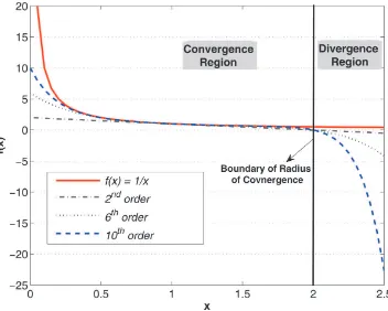
Figure 1. Taylor approximations forf(x)= 1
x. This figure plots the functionf(x)=
1
xand presents 2nd-, 6th-, and 10th-order approximations
around the interval ( ¯x−r,x¯+r)=(0,2.5), ¯x=1. The online version of this figure is in color.
The cubic approximation of the SDF in (5) aroundgt is given by
mt =βg
−γ t
1+1
2γ(γ+1) 1
K
K
k=1
g k,t
gt
−1 2
−1
6γ(γ+1)(γ+2) 1
K
K
k=1
g k,t
gt
−1 3
. (7)
Equation (6) is the function of the cross-sectional mean and cross-sectional variance, while Equation (7) is the function of the first two moments and cross-sectional skewness. These two equations set the base for our second empirical investigation. By testing (6) we test whether the second moment only can explain the cross-sectional variation of the pricing kernel. By testing (7) we test whether second and third moments of the sectional consumption growth can jointly explain the cross-sectional variation.
The approximations in (6) and (7) should be close enough to the SDF given in (5). Calin, Chen, Cosimano, and Himonas (2005) were among the first to highlight the importance of the accuracy of approximation schemes in asset pricing models and of the region for which such approximations are feasible. In general, it is important to identify the convergence interval (x0−
r, x0+r) of the Taylor series expansion around the pointx0with
the radius of convergence r. For a Taylor series, the radius of convergence is the distance between the approximation point and the closest singularity of the function. For example, for a CRRA utility function the marginal utility is given byc−γ
, where γ is the RRA coefficient. Clearly, marginal utility has
a singularity at zero, which implies that, if we approximate marginal utility around a point c, the radius of convergence is given byc, preventing the use of data outside the interval (0,2c). Example 1 illustrates this point analytically. Example 2 underscores how observations outside the convergence interval can lead to undesirable properties of the function of interest, namely, negative SDF. We illustrate this empirical problem using BCG example.
Example 1. Consider the marginal utility of a myopic in-vestor f(x)= 1x and approximate it around the point x=1. The radius of convergence in this case isr=1, and we expect the Taylor series to converge absolutely to the true function in the interval (0,2). Figure 1 plots the functionf(c) as a solid line and its second-, sixth-, and tenth-order approximations as dashed lines over the interval (0,2.5). When the approximation order increases, the approximated function converges to the true functionf(x) in the region of convergence. However, in the divergence region in the figure (x >2) the opposite is true: when approximation order increases, the approximate function diverges from the true function as the approximation order in-creases and the approximation becomes unreliable. Odd-power approximations show a similar divergence pattern (not reported to preserve clarity in Figure 1).
Example 2. We implement BCG sample selection filters for individual CEX data and show that even this careful filter-ing might lead to the “blow-up” of the SDF resultfilter-ing in the high volatility SDF albeit with a negative marginal utility. BCG
calibrated the following equation:
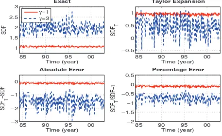
wheregi,t is the individual consumption growth andgt is the cross-sectional average over the individual household consump-tion growth rates. Figure 2(a) showsmt given above for two levels of γ. Figure 2(a) top right panel demonstrates thatmt has high volatility forγ =3, but it comes at a cost of having a negative marginal utility. The problem would worsen with higher levels ofγ. On the contrary, Figure 2(b) demonstrates that using clusters instead of individual data, we obtain positive SDF everywhere.
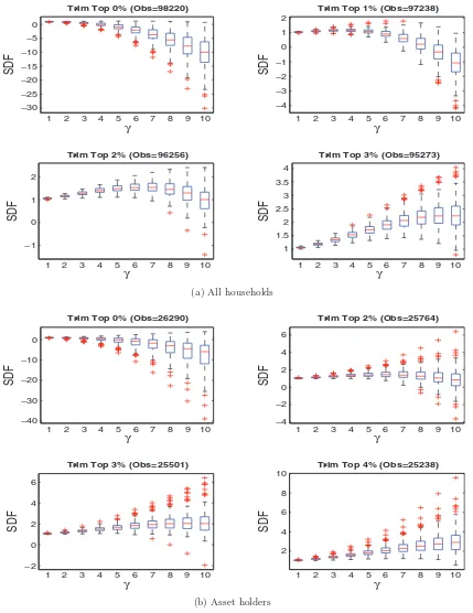
In Example 2, we do not filter by asset holders in order to make samples comparable across ours and BCG approach, but the same negative marginal utility graphs are obtained in BCG case when we filter by asset holders. These two examples em-phasize that empirical researchers should be careful when work-ing with approximations so the results remain economically meaningful. In particular, we show that the radius of conver-gence for Taylor approximations (6) and (7) should not be vio-lated, especially for high enough values ofγ.Figure 3presents boxplots of the consumption growth rates distribution used to obtain cubic approximations in Equation (7) as a function of
γ. Each graph applies a different level of trimming to the data before computing Equation (7). The plots show that, in order to get approximations everywhere positive for reasonable levels of
γ, at least 3% of the right tail of the distribution of consumption growth rates needs to be trimmed (Figure 3(a)). This trimming needs to increase to 4% if only asset holders are considered (Figure 3(b)).
3. EMPIRICAL METHODOLOGY AND DATA
In this section we briefly describe the CEX dataset house-hold selection criteria, the methods for constructing househouse-hold cohorts and clusters, and the asset returns data used.
3.1 The Consumer Expenditure Survey (CEX)
The CEX is produced by the Bureau of Labor Statistics (BLS). The CEX provides a continuous flow of information on the buying habits of American consumers and furnishes data to support periodic revisions of the Consumer Price Index (CPI) market basket of goods and services and their relative impor-tance. Using a stratified sample methodology, the BLS designs the survey to be representative of the U.S. civilian population. This dataset is not a proper panel, but rather a series of cross-sections with a limited time dimension. The data are organized in quarterly files. Approximately 5000 households are inter-viewed three months apart for five consecutive quarters (a trial interview is conducted in the first quarter). These interviews are staggered evenly throughout the year on a monthly basis and households report their consumption over three months
preced-ing the interview. Attanasio and Weber (1995) and Attanasio and Davis (1996) provided further details about CEX dataset.
For each interview, respondents report consumption over the previous quarter and provide the reference month in which expenditures took place. In theory, this enables us to have up to 12 months of consumption information for each house-hold, making it possible to obtain monthly consumption series. However, careful inspection of the data indicates that monthly reported consumption is most often equal to quarterly tion divided by 3. For this reason, we use quarterly consump-tion measured monthly. The sample period in our study covers interviews conducted from January 1984 to December 2002, re-sulting in 219 monthly cross-sections of household interviews.
3.2 Definition of Nondurables and Services (NDS)
We calculate per capita quarterly nondurable and services (NDS) consumption by aggregating data in the following CEX categories: food, alcoholic beverages, tobacco, gas, utilities, apparel, public transportation, household operations, personal care, entertainment (only fees and admissions), education, read-ing, life and other personal insurance, and health care. This def-inition of NDS is consistent with the defdef-inition in BCG and is broader than the definition adopted by Jacobs and Wang (2004), which ignores the last five terms listed above. Gift items are ex-cluded from aggregation. Per capita consumption is obtained by dividing each household consumption by the number of house-hold members. Nominal consumption is corrected for inflation using the seasonally unadjusted CPI level obtained from Center for Research in Security Prices (CRSP; variable CPIIND from crsp.mcti file) and follows Balduzzi and Yao (2007).
3.3 Household Selection Criteria
We drop households for which the reference person’s age is below 18 or above 75 years (Attanasio and Weber1995) and if food consumption is not positive (e.g., BCG and Balduzzi and Yao2007). Following BCG, we adopt a three-stage consumption growth filter. First, we require households to report consump-tion for at least three consecutive periods. Second, we drop
ci,t/ci,t−1, ifci,t/ci,t−1iseitherbelow (1/5)orabove 5. Third,
we dropci,t/ci,t−1ifci,t/ci,t−1<(1/2)andci,t+1/ci,t>2. Note that the second filter is slightly stronger than the filter originally proposed by BCG (who did not imposed a lower bound) and is consistent with Balduzzi and Yao (2007). This strengthening of the second filter is necessary to ensure a meaningful SDF because it avoids the need to take negative powers of very small numbers.
3.4 Data Partition: Cohorts and Clusters
To reduce measurement errors and to improve the approx-imation of the Taylor series expansion of the aggregate SDF, we partition households into groups based on observable demo-graphic characteristics. Organizing households by similar edu-cation, age, and income characteristics, we implicitly assume that a representative agent exists within each group. One issue with this approach is that the choice of grouping method for the construction of synthetic cohorts is not obvious. On one hand,
85 90 95 00
1 1.5 2 2.5 3
Time (year)
SDF
Exact
γ=1 γ=3
85 90 95 00
−0.5 0 0.5 1
Time (year)
SDF
T
Taylor Expansion
85 90 95 00
−3 −2 −1 0
Time (year)
SDF
T
−SDF
Absolute Error
85 90 95 00
−2 −1.5 −1 −0.5 0 0.5
Time (year)
SDF
T
/SDF−1
Percentage Error
(a) With individual households (BCG 2002)
85 90 95 00
1 1.5 2
Time (year)
SDF
Exact
γ=1 γ=3
85 90 95 00
1 1.5 2
Time (year)
SDF
T
Taylor Expansion
85 90 95 00
−0.4 −0.2 0 0.2 0.4
Time (year)
SDF
T
−SDF
Absolute Error
85 90 95 00
−0.4 −0.2 0 0.2 0.4
Time (year)
SDF
T
/SDF−1
Percentage Error
(b) With clusters
Figure 2. Third-order approximation of the Stochastic Discount Factor (SDF). The figure reports the SDF (8), its third power Taylor
approximation (7), and both the absolute and percentage error of the approximation. Panel A refers to the SDF in Brav, Constantinides, and
Geczy (2002), which is based on all households’ consumption data; BCG filters are imposed. Panel B presents a cluster-based SDF, which is based
on 12 clusters,K=12. Time–discount factorβ=1 in both figures. RRA coefficients areγ =1,3. Sample period is March 1984–November
2002. The online version of this figure is in color.
−30 −25 −20 −15 −10 −5 0
1 2 3 4 5 6 7 8 9 10
γ
Trim Top 0% (Obs=98220)
SDF
−4 −3 −2 −1 0 1 2
1 2 3 4 5 6 7 8 9 10
γ
Trim Top 1% (Obs=97238)
SDF
−1 0 1 2
1 2 3 4 5 6 7 8 9 10
γ
Trim Top 2% (Obs=96256)
SDF
1 1.5 2 2.5 3 3.5 4
1 2 3 4 5 6 7 8 9 10
γ
Trim Top 3% (Obs=95273)
SDF
(a) All households
−40 −30 −20 −10 0
1 2 3 4 5 6 7 8 9 10 γ
Trim Top 0% (Obs=26290)
SDF
−4 −2 0 2 4 6
1 2 3 4 5 6 7 8 9 10 γ
Trim Top 2% (Obs=25764)
SDF
−2 0 2 4 6
1 2 3 4 5 6 7 8 9 10 γ
Trim Top 3% (Obs=25501)
SDF
2 4 6
8
10
1 2 3 4 5 6 7 8 9 10 γ
Trim Top 4% (Obs=25238)
SDF
(b) Asset holders
Figure 3. Approximated SDF as a function ofγ .Distributions of approximated SDF as a function ofγand for various levels of trimming.
The top panel presents results for all households; the bottom panel filters out nonmarket participants. The online version of this figure is in color.
one does not want the groups to be too small, because in that case measurement error and random effects will be very large. On the other hand, if groups are too large, it may not be appro-priate to assume the existence of a representative agent in each cohort.
We propose two methods to group households. The first method is similar to the method proposed by Jacobs and Wang (2004) who partitioned households into several age and
edu-cation groups. To better control for households heterogeneity, we add an income dimension to the partition. We use the CEX variable “FINCBTAX,” which is defined as total household in-come before taxes in the previous 12 months. Given that this variable is recorded only in the first and fourth quarter, we set the income variable in the second and third quarter equal to the income in the first quarter. To implement the partition, we group households into three education categories: at most
a high-school diploma; some college experience; and at least a bachelor degree. For each education group, we consider at most three age groups and, within each age group, at most three income groups. The cutoffs in the subgroups are the median and terciles depending on whether we have one or two cutoffs. This partition generates as few as three (education) groups and as many as 27 education–age–income groups (3×3×3).
The second method is based on clustering analysis. Cluster-ing analysis aims to partitionnobservations intoKgroups, or clusters, that are as far away as possible from each other, but con-taining observations that are as homogenous as possible within each cluster with respect to certain prespecified characteristics of the data. If we measure distance with an L2 (Euclidean) norm, we end up with a so calledk-means model that can be quite sen-sitive to outliers. If we choose an L1 norm, the effect of outliers can be mitigated. We exploit both features of the procedure to first identify outliers and subsequently eliminate their impact on the final clusters. To implement our clustering analysis, we use the SAS FASTCLUS procedure. A general formulation for constructingKclusters is described in the following algorithm:
Step 1. Choose the number of clusters,K.
Step 2. Choose arbitrarily an initial set ofK random points (centroids) from the sample as cluster centers:
m(1)1 , . . . , m(1)K.
Step 3. Assign each observation in the sample to the clus-ter with the closest mean, so the clusclus-ter Si(1), i=
Step 5. Repeat Steps 3 and 4 until the convergence criteria are met: usually this means that the assignment and cluster centers have not changed.
Mirkin (2005) provided a detailed description of theK-means algorithm (see Chapter 3 in his book).
Our objective is to partition the CEX data into clusters along three dimensions (age, education, and income) and compute consumption growth for each one of these clusters. We perform our clustering analysis on each monthly cross-section of house-hold data. To that end, we take the following steps. First, we standardize the data to have mean zero and unit standard devi-ation to ensure that variables with high variance are not driving our results. Second, we partition data into 50 clusters using the L2 norm in order to identify likely cluster-outliers, which con-tain just one observation. We eliminate these clusters and use the remaining clusters as the initial seeds for the next use of the clustering procedure. Using 75 or 100 clusters as preliminary partition does not make much difference. Next, we recompute clusters using an L1 norm in order to mitigate the impact of out-liers on the identification of clusters. Finally, we compute the consumption growth of each cluster by taking the ratio of av-erage consumption and avav-erage lagged consumption, where the average is taken for the members of each cluster. This process is repeated for several data partitions.
The definition of cohort/cluster-based consumption growth deserves some explanation. We do not aggregate over consump-tion growth in a given group, but rather aggregate the levels of consumption within a cohort. We then compute consumption growth for the group as the ratio of the aggregate levels. This ap-proach is consistent with the existence of additive measurement errors in consumption (see Balduzzi and Yao2007for details). Formally, per capita consumption of a representative cohortkat timetis given by
whereNk,tis the number of observations in cohortkin month
t. We define cohort consumption growth as the ratio of two consecutive per capita consumption levels (10):
gk,t =
ck,t
ck,t−1
. (11)
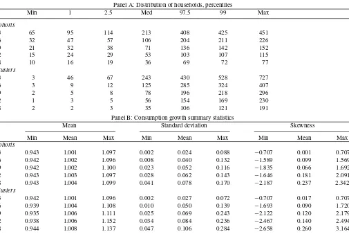
Table 1 reports the pooled distribution (percentiles) of the size of the groups (Panel A) and descriptive statistics on the consumption growth of the members of such groups (Panel B). We report results for 3, 6, 9, 12, and 18 cohorts and clusters. The three cohorts’ case represents three education cohorts; six cohorts’ case corresponds to a data partition on three education and two age cohorts; nine cohorts’ case—three education and three age groups’ partition; 12 cohorts’ case—three education, two income, and two age groups; and, finally, 18 cohorts’ case— three education, three income, and two age groups’ partition of the data.
Comparing cohorts to clusters, it is apparent that observa-tions in cohorts are more evenly spaced than those in clusters. By construction, cohort boundaries are the percentiles of the distribution of age, income, and education. The clustering pro-cedure assigns observations to groups using similarity among the observations with respect to age, education, and income char-acteristics as the main criterion. Hence the size of the clusters is likely to be relatively skewed and it should not be surprising that we occasionally find small clusters. Panel A reveals that very small clusters (with size less or equal than 2) are extremely rare. Even for the partition with 18 clusters per month, totaling 3942 clusters (18×219), at most 40 cluster-month observations have a size less than or equal to 2.
Panel A ofTable 1presents the tiseries minimum, me-dian, and maximum of the cross-sectional moments of cohort-and cluster-based consumption growth. As it can be seen, the cross-sectional moments obtained via clustering point out to more heterogeneity across clusters than across cohorts. This difference is stronger for finer partitions (higherk). For exam-ple, consumption growth volatility is higher in clusters than in cohorts. Panel B ofTable 1 shows that forK=18, the aver-age cross-sectional volatility is 0.106 for clusters and 0.078 for cohorts.
3.5 Asset Returns
We consider value and equally weighted market returns that include capital gains and dividends on the pool of stocks traded on NYSE, AMEX, and NASDAQ. The risk-free rate
Table 1. CEX data summary statistics
Panel A: Distribution of households, percentiles
Min 1 2.5 Med 97.5 99 Max
Cohorts
3 65 95 114 213 408 425 451
6 32 47 57 106 204 211 226
9 21 32 38 71 136 142 152
12 15 24 29 53 103 107 115
18 10 16 19 36 69 72 77
Clusters
3 3 46 67 243 430 528 727
6 3 9 12 125 285 324 407
9 2 5 8 78 196 218 296
12 1 3 5 56 154 169 230
18 2 2 3 35 106 121 191
Panel B: Consumption growth summary statistics
Mean Standard deviation Skewness
Min Mean Max Min Mean Max Min Mean Max
Cohorts
3 0.943 1.001 1.097 0.002 0.024 0.088 −0.707 0.001 0.707
6 0.942 1.002 1.096 0.008 0.040 0.132 −1.589 0.099 1.569
9 0.942 1.002 1.100 0.023 0.052 0.116 −1.835 0.066 1.692
12 0.943 1.003 1.097 0.028 0.062 0.143 −1.646 0.181 2.091
18 0.943 1.004 1.099 0.041 0.078 0.170 −2.187 0.237 2.342
Clusters
3 0.942 1.001 1.096 0.002 0.027 0.072 −0.707 0.017 0.707
6 0.939 1.004 1.108 0.010 0.050 0.139 −1.693 0.090 1.720
9 0.935 1.006 1.111 0.025 0.069 0.243 −2.122 0.120 2.179
12 0.938 1.006 1.152 0.034 0.084 0.236 −2.467 0.140 2.494
18 0.944 1.008 1.137 0.047 0.106 0.284 −2.658 0.260 3.164
Panel A presents descriptive statistics for the number of households within cohorts/clusters considered. Both cohorts and clusters are formed on education, age, and income characteristics. Cohorts are formed according to the exogenous criteria. Clusters are formed according to endogenous criteria using theK-means clustering method. The exact description of the cohorts/clusters is discussed in Section 3.2. Column 1 in each panel represents the number of cohorts/clusters into which households are sampled. Columns 2–4 report the time-series minimum, median, and maximum number of households falling in each cohort. Columns 5–8 present the median of the 1%, 2.5%, 97.5%, and 99% percentiles across cohorts/clusters. Panel B presents descriptive statistics for household consumption growth. Columns 2–4 present the time-series minimum, mean, and maximum of the cross-sectional mean of the cohort-based consumption growth. Columns 5–7 present the time-series minimum, mean, and maximum of the cross-sectional cohort-based consumption growth standard deviation. Columns 8–10 present the time-series minimum, mean, and maximum of the cross-sectional cohort-based consumption growth skewness. The sample period is from March 1984 to November 2002. The data is quarterly sampled at monthly frequency.
is the monthly return on a 30-day Treasury Bill portfolio. Returns are deflated using the seasonally unadjusted inflation rate obtained from the Consumer Price Index for All Urban Consumers. The returns are from March 1984 to November 2002. Market returns, risk-free rate, and CPI data are obtained from the CRSP via Wharton Research Data Base. We compute quarterly returns by compounding monthly returns. Table 2
presents summary statistics for quarterly real asset returns. The returns are overlapping and available at a monthly frequency to
match consumption growth. All returns are from March 1984 to November 2002, resulting in 219 monthly observations.
4. EMPIRICAL ANALYSIS
In this section, we present empirical results. In Section 4.1, we discuss results related to testing unapproximated Euler Equation (5). We discuss approximations (6) and (7) in Section 4.2, and robustness checks in Section 4.3.
Table 2. Summary statistics for asset returns
Central moments Autocorrelations
Assets Mean SD Skew Kurt Lag 1 Lag 2 Lag 3 Lag 4
Risk-free rate 0.005 0.005 0.311 4.327 0.784 0.484 0.292 0.284
VW market return 0.021 0.081 –0.671 4.492 0.643 0.216 –0.150 –0.141
EW market return 0.020 0.104 –0.349 4.011 0.682 0.195 –0.204 –0.259
The returns are overlapping and available at a monthly frequency to match consumption growth. We report means, standard deviations (SD), skewness, and kurtosis for the equally weighted (EW) and value weighted (VW) market returns and for the risk-free rate. The market return is the return on the aggregate value-weighted NYSE-AMEX-NASDAQ index. The risk-free rate is the monthly return on 30-day Treasury Bill Portfolio (CRSP variable T30RET). In addition to the first four moments, we also report the first four autocorrelations for market returns and the risk-free rate. The sample period is from March 1984 to November 2002.
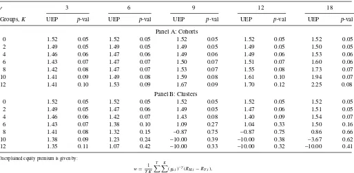
Table 3. Unexplained equity premium, equally weighted SDF
γ 3 6 9 12 18
Groups,K UEP p-val UEP p-val UEP p-val UEP p-val UEP p-val
Panel A: Cohorts
0 1.52 0.05 1.52 0.05 1.52 0.05 1.52 0.05 1.52 0.05
2 1.49 0.05 1.49 0.05 1.49 0.05 1.49 0.05 1.50 0.05
4 1.46 0.06 1.47 0.06 1.49 0.06 1.49 0.06 1.53 0.06
6 1.43 0.07 1.47 0.07 1.50 0.07 1.51 0.07 1.60 0.06
8 1.42 0.08 1.47 0.07 1.53 0.07 1.55 0.08 1.73 0.07
10 1.41 0.09 1.49 0.08 1.59 0.08 1.61 0.10 1.94 0.07
12 1.41 0.10 1.53 0.09 1.67 0.09 1.70 0.12 2.25 0.08
Panel B: Clusters
0 1.52 0.05 1.52 0.05 1.52 0.05 1.52 0.05 1.52 0.05
2 1.49 0.05 1.47 0.06 1.49 0.05 1.47 0.06 1.51 0.05
4 1.46 0.06 1.42 0.07 1.43 0.08 1.40 0.09 1.54 0.07
6 1.43 0.07 1.38 0.10 1.09 0.27 1.04 0.33 1.50 0.16
8 1.41 0.08 1.32 0.15 –0.87 0.75 –0.87 0.75 0.86 0.66
10 1.38 0.09 1.23 0.24 –10.00 0.39 –10.00 0.38 –3.67 0.62
12 1.35 0.11 1.07 0.42 –10.00 0.33 –10.00 0.32 –10.00 0.41
Unexplained equity premium is given by:
w= 1
T K T
t=1 K
k=1
(gk,t)−γ(RM,t−RF,t),
whereKis the number of household groups, either cohorts (Panel A) or clusters (Panel B),gk,tis the cohort(cluster)-based consumption growth, Panel A(B) presents results for equally weighted SDF constructed using cohort-(cluster-)based consumption growth, respectively. The unexplained equity premium (uep) reported as−10 means that theuepis less than−10 at the corresponding level of the RRA. Thep-values are based on 3-lag Newey-West adjusted standard errors. The results are based on the value-weighted equity premium. The sample period is from March 1984 to November 2002. Observations are quarterly at a monthly frequency.
4.1 Unexplained Equity Premium
First, we test the hypothesis (5) that the equally weighted average of the cohort-based marginal rates of substitution is a valid SDF. Specifically, we test whether the following statistic
wis equal to zero:
w= 1
T K
T
t=1
K
k=1
(gk,t)−γ(RM,t−RF,t). (12) The statisticwin (12) represents the sample unexplained equity premium in our model. Table 3presents the estimates of (12) for various sets of cohorts and clusters. Following Brav, Con-stantinides, and Geczy (2002), we setβ =1 in our tests. Panel A presents cohort-basedwestimates along with theirp-values; Panel B presents cluster-basedwestimates along with theirp -values. All results reported in the paper are based on the value-weighted premium. We obtain similar results for the case of the equally weighted premium. The p-value ofw=0 against an unspecified alternative is computed based on thet-statistic. By construction, consumption growth and return observations are overlapping. Therefore,t-statistics and p-values are corrected for autocorrelation. We have used the Newey-West correction with three lags in order to account for the auto-correlation within clusters. The observations across clusters are independent. Risk aversion coefficient is varied between 0 and 12.
γ =0 (first row in all panels) corresponds to the quarterly sample average of the equity premium in our sample, equal to 1.52% per quarter. Panel A ofTable 3shows that we reject a zero unexplained equity premium for anyγ >0 and any number of cohorts on the 10% level of statistical significance. 12 cohorts,
γ ≥11 represents the exception, but this result is not econom-ically meaningful becauseuepis increasing, not decreasing in this case. In fact, for most of cohorts,wis increasing, not de-creasing. Intermediate cases forK (not reported) provide the same result.
The situation is different when we testw=0 for the cluster-based SDF (Panel B of Table 3). We cannot reject that the equity premium is zero any more for certain sets of clusters and certain values ofγ. The unexplained equally weighted equity premium estimates cross zero for values ofγ between 5 and 7 andK=9,12,and 18. As the case ofK=3 shows, this result does not hold if one uses too few clusters for the SDF con-struction: although Newey-West correctedp-values are slightly higher than 0.10,uepnever crosses zero. For higherK, we can-not reject a zero equity premium forγ coefficients between 5 and 7. Malloy, Moskowitz, and Vissing-Jørgensen (2009), us-ing the consumption of stockholders only from the CEX dataset and 25 Fama-French portfolios, estimated the RRA coefficient to be around 10. Our estimates are closer to theirs than to Brav, Constantinides, and Geczy (2002). These authors matched the equity premium in their setting with a lower value ofγ =3 or 4. Example 2 andFigure 2point out a reason—their SDF is more volatile than ours, albeit negative.
These simple tests show that idiosyncratic consumption risk indeed helps to explain the equity premium with reasonable values of the RRA coefficient when sufficiently many clus-ters generate enough cross-sectional distribution variation. The cross-sectional variation in income seems to play an impor-tant role here. Indeed, we fail to reject the hypothesis that the equally weighted average of the cluster-based IMRS is a
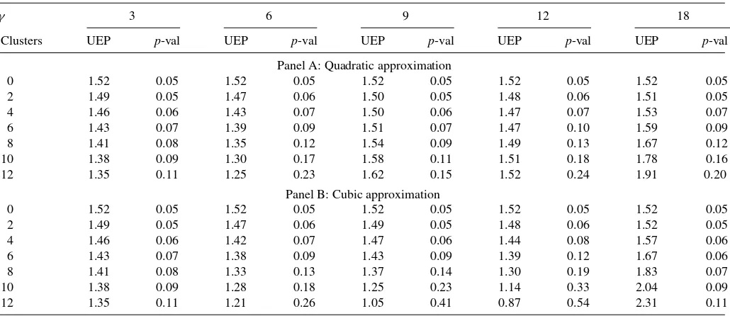
Table 4. Unexplained equity premium. Equally weighted SDF, approximations
γ 3 6 9 12 18
Clusters UEP p-val UEP p-val UEP p-val UEP p-val UEP p-val
Panel A: Quadratic approximation
0 1.52 0.05 1.52 0.05 1.52 0.05 1.52 0.05 1.52 0.05
2 1.49 0.05 1.47 0.06 1.50 0.05 1.48 0.06 1.51 0.05
4 1.46 0.06 1.43 0.07 1.50 0.06 1.47 0.07 1.53 0.07
6 1.43 0.07 1.39 0.09 1.51 0.07 1.47 0.10 1.59 0.09
8 1.41 0.08 1.35 0.12 1.54 0.09 1.49 0.13 1.67 0.12
10 1.38 0.09 1.30 0.17 1.58 0.11 1.51 0.18 1.78 0.16
12 1.35 0.11 1.25 0.23 1.62 0.15 1.52 0.24 1.91 0.20
Panel B: Cubic approximation
0 1.52 0.05 1.52 0.05 1.52 0.05 1.52 0.05 1.52 0.05
2 1.49 0.05 1.47 0.06 1.49 0.05 1.48 0.06 1.52 0.05
4 1.46 0.06 1.42 0.07 1.47 0.06 1.44 0.08 1.57 0.06
6 1.43 0.07 1.38 0.09 1.43 0.09 1.39 0.12 1.67 0.06
8 1.41 0.08 1.33 0.13 1.37 0.14 1.30 0.19 1.83 0.07
10 1.38 0.09 1.28 0.18 1.25 0.23 1.14 0.33 2.04 0.09
12 1.35 0.11 1.21 0.26 1.05 0.41 0.87 0.54 2.31 0.11
This table presents the unexplained equity premium (12) and the correspondingp-values for different sets of household clusters sorted on education, age, and income. Panel A(B) reports the unexplained equity premium based on the quadratic (cubic) approximation of the SDF given by Equation (6) and (7) in Section 2.2. Thep-values are based on 3-lag Newey-West adjusted standard errors. The results are based on the value-weighted equity premium. The sample period is from March 1984 to November 2002. Observations are quarterly at a monthly frequency.
valid SDF for “endogenous” clusters constructed by educa-tion, age, and income characteristics. We find that 9–18 clus-ters provide a good balance between the amount of hetero-geneity and some reduction in the measurement error con-tained in the CEX dataset. This result cannot be reproduced using “exogenous” cohort groupings based on the same demo-graphic characteristics. This empirical result provides an im-portant insight on the amount of incomplete risk sharing in the economy. It suggests that risk sharing within the clusters is greater than across the clusters for a sufficiently large number of clusters.
The results inTable 3are based on the fitting of the excess market return alone. We have also run a formal GMM estimation of Equation (5) using gross market return and risk-free rate since risk-free rate and equity premium puzzle are tightly connected under CRRA specification. GMM estimation produces sharp and economically reasonable estimates ofβ andγ: ˆβ =0.96 (t-stat=–4.71), ˆγ =5.19 (t-stat =11.34). Nevertheless, the model is rejected for both cohorts and clusters on all levels of statistical significance. The fit of the model is slightly better for cluster-based than cohort-based SDF. Overall, GMM estimation shows the limitation of this framework to explain simultaneously risk-free and equity premium puzzles.
4.2 Taylor Approximations
In the next section, we use Taylor series approximations to study which moments of the cross-sectional consumption growth drive our results. The results are presented inTable 4. First, neither quadratic nor cubic Taylor approximations of the cohort-based SDF can explain the equity premium irrespective of the γ coefficient. We reject w=0 hypothesis everywhere in this case, consistent with the evidence in Panel A,Table 3
(cohort-based approximations are not reported for the sake of space). This result reconfirms that demographic cohorts con-structed “exogenously” do not provide necessary cross-sectional variation present in the data, as descriptive statistics of the data suggests (seeTable 1). Such cohort-based finding remains at odds with Brav, Constantinides, and Geczy (2002), who concluded that the skewness of the cross-sectional distribution of consumption growth is an important factor in explaining the equity premium. Second, Panel A ofTable 4indicates that first and second cross-sectional moments are not enough to explain the equity premium (12) even for a cluster case. Third, the cubic approximation (7) yields a better fit but it does not cross zero for any number of clusters that we report here. Although thew
estimates do not cross zero, they are not significantly different from it. We obtain a cubic approximation to be more exact in the case of the equally weighted equity premium:uep=0 for
γ ≈11 forK=9 and 12. As can be seen from Equation (7), for a Taylor approximation of the SDF to be successful, correlation of market return with cross-sectional mean and skewness should be positive, while the correlation of the cross-sectional variance with market return should be negative. Indeed, cluster-based correlations for six and nine clusters achieve exactly this. At the same time, we observe that cohort-based correlations do not follow this pattern (results are not reported for space consideration, but available upon request from the authors).
Results of Tables 3 and 4, therefore, can be summarized by three robust empirical findings. First, in our sample, the cluster-based SDF is consistent with the historical U.S. eq-uity premium, while the cohort-based SDF is not. Second, cross-sectional skewness of the cluster-based distribution of consumption growth plays a key role in explaining the equity premium with a reasonable risk aversion coefficient. Third, in order to obtain this effect, we need to consider sufficiently many
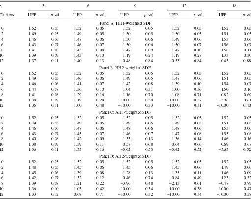
Table 5. Unexplained equity premium. Alternative weighting schemes
γ 3 6 9 12 18
Clusters UEP p-val UEP p-val UEP p-val UEP p-val UEP p-val
Panel A: HH1-weighted SDF
0 1.52 0.05 1.52 0.05 1.52 0.05 1.52 0.05 1.52 0.05
2 1.49 0.05 1.49 0.05 1.50 0.05 1.50 0.05 1.51 0.05
4 1.46 0.06 1.47 0.06 1.50 0.06 1.49 0.06 1.53 0.06
6 1.43 0.07 1.46 0.07 1.50 0.06 1.50 0.07 1.56 0.07
8 1.41 0.08 1.45 0.08 1.47 0.09 1.47 0.10 1.58 0.11
10 1.39 0.09 1.43 0.10 1.19 0.24 1.19 0.27 1.33 0.30
12 1.37 0.11 1.40 0.13 –0.48 0.84 –0.53 0.84 –0.43 0.88
Panel B: HH2-weighted SDF
0 1.52 0.05 1.52 0.05 1.52 0.05 1.52 0.05 1.52 0.05
2 1.49 0.05 1.46 0.06 1.49 0.05 1.47 0.06 1.51 0.05
4 1.46 0.06 1.41 0.07 1.42 0.08 1.39 0.10 1.54 0.07
6 1.44 0.07 1.36 0.10 1.04 0.31 1.00 0.36 1.50 0.16
8 1.41 0.08 1.29 0.16 –1.16 0.70 –1.08 0.71 0.82 0.69
10 1.38 0.09 1.19 0.28 –10.00 0.38 –10.00 0.37 –3.96 0.61
12 1.35 0.11 1.00 0.48 –10.00 0.33 –10.00 0.31 –10.00 0.40
Panel C: AH1-weighted SDF
0 1.52 0.05 1.52 0.05 1.52 0.05 1.52 0.05 1.52 0.05
2 1.49 0.05 1.49 0.05 1.49 0.05 1.49 0.05 1.51 0.05
4 1.46 0.06 1.47 0.06 1.48 0.06 1.48 0.06 1.53 0.06
6 1.43 0.07 1.45 0.07 1.46 0.07 1.47 0.08 1.55 0.08
8 1.40 0.08 1.42 0.09 1.33 0.13 1.36 0.14 1.46 0.16
10 1.38 0.09 1.39 0.11 0.57 0.68 0.64 0.66 0.69 0.67
12 1.36 0.11 1.33 0.16 –3.62 0.50 –3.42 0.52 –3.63 0.52
Panel D: AH2-weighted SDF
0 1.52 0.05 1.52 0.05 1.52 0.05 1.52 0.05 1.52 0.05
2 1.48 0.05 1.45 0.06 1.45 0.06 1.45 0.06 1.49 0.06
4 1.45 0.06 1.39 0.08 1.28 0.13 1.35 0.11 1.46 0.09
6 1.42 0.07 1.32 0.12 0.46 0.74 0.84 0.49 1.23 0.32
8 1.39 0.08 1.21 0.22 –3.96 0.48 –2.13 0.61 –0.47 0.89
10 1.36 0.10 1.03 0.42 –10.00 0.34 –10.00 0.38 –10.00 0.47
12 1.33 0.12 0.68 0.71 –10.00 0.32 –10.00 0.34 –10.00 0.38
This table presents the unexplained equity premium and the correspondingp-values for different sets of household clusters sorted on education, age, and income. Unexplained equity premium is given by:
w= 1
T T
t=1 K
k=1
ωk,t×(gk,t)−γ(RM,t−RF,t),
whereKis the number of household clusters,gk,tis the cluster-based consumption growth,RM,t−RF,tis the value-weighted excess market return. Panel A(B) presents results for the
HH1(HH2)-weighted SDF, where the weighting scheme favors clusters with more (fewer) households within each cluster. Panel C(D) presents results for the AH1(AH2)-weighted SDF, where the weighting scheme favors clusters with higher number (fraction) of asset holders within each cluster. The unexplained equity premium (uep) reported as−10 means that theuep
is less than−10 at the particular level of the RRA. Thep-values are based on 3-lag Newey-West adjusted standard errors. The results are based on the value-weighted equity premium. The sample period is from March 1984 to November 2002. Observations are quarterly at a monthly frequency.
clusters of similar households, so enough cross-sectional varia-tion is generated.
4.3 Alternative Weighting Schemes
The Euler equation (5) applies an equally weighted average scheme to the cluster-based SDFs. However, the theory does not preclude the use of alternative weighting schemes. We verify the robustness of our results by applying four alternative weighting schemes for cluster-based SDF. Weighting schemes HH1 and HH2 are based on the number of households in the clusters. Weighting schemes AH1 and AH2 are based on the number of
asset holders in the clusters. Formally, we define these weighting schemes as follows:
HH1 weighting schemefavors clusters with ahighernumber of households in them. Thus, the weightwHH1k,t for clusterkin monthtis computed as a fraction of households in clusterkwith respect to the total number of households available in montht:
wHH1k,t =HHk,t
HHt . (13)
HH2 weighting scheme favors clusters with a lower number of households in them. Thus, the weightwHH2k,t for clusterkin
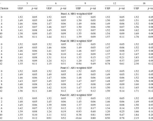
Table 6. Unexplained equity premium. Alternative weighting schemes, cubic approximation
γ 3 6 9 12 18
Clusters UEP p-val UEP p-val UEP p-val UEP p-val UEP p-val
Panel A: HH1-weighted SDF
0 1.52 0.05 1.52 0.05 1.52 0.05 1.52 0.05 1.52 0.05
2 1.49 0.05 1.49 0.05 1.50 0.05 1.50 0.05 1.51 0.05
4 1.46 0.06 1.47 0.06 1.49 0.06 1.49 0.06 1.52 0.06
6 1.43 0.07 1.46 0.07 1.50 0.06 1.50 0.07 1.56 0.06
8 1.41 0.08 1.45 0.08 1.52 0.07 1.52 0.08 1.62 0.07
10 1.38 0.09 1.45 0.09 1.55 0.08 1.54 0.09 1.69 0.08
12 1.36 0.11 1.44 0.11 1.59 0.09 1.57 0.11 1.78 0.09
Panel B: HH2-weighted SDF
0 1.52 0.05 1.52 0.05 1.52 0.05 1.52 0.05 1.52 0.05
2 1.49 0.05 1.46 0.06 1.49 0.05 1.47 0.06 1.52 0.05
4 1.46 0.06 1.41 0.07 1.46 0.07 1.43 0.08 1.57 0.06
6 1.44 0.07 1.36 0.10 1.42 0.09 1.37 0.12 1.67 0.06
8 1.41 0.08 1.31 0.14 1.35 0.15 1.27 0.21 1.83 0.07
10 1.38 0.09 1.24 0.21 1.20 0.27 1.09 0.37 2.05 0.09
12 1.35 0.11 1.15 0.31 0.94 0.49 0.78 0.61 2.30 0.12
Panel C: AH1-weighted SDF
0 1.52 0.05 1.52 0.05 1.52 0.05 1.52 0.05 1.52 0.05
2 1.49 0.05 1.49 0.05 1.49 0.05 1.49 0.05 1.51 0.05
4 1.46 0.06 1.47 0.06 1.48 0.06 1.48 0.06 1.52 0.06
6 1.43 0.07 1.45 0.07 1.47 0.07 1.48 0.07 1.56 0.06
8 1.40 0.08 1.43 0.08 1.47 0.08 1.49 0.09 1.60 0.08
10 1.38 0.09 1.42 0.10 1.47 0.10 1.50 0.11 1.65 0.09
12 1.36 0.11 1.40 0.12 1.47 0.12 1.50 0.14 1.71 0.12
Panel D: AH2-weighted SDF
0 1.52 0.05 1.52 0.05 1.52 0.05 1.52 0.05 1.52 0.05
2 1.48 0.05 1.45 0.06 1.45 0.06 1.46 0.06 1.49 0.05
4 1.45 0.06 1.39 0.08 1.37 0.09 1.41 0.08 1.50 0.07
6 1.42 0.07 1.32 0.12 1.22 0.17 1.34 0.14 1.55 0.10
8 1.39 0.08 1.24 0.19 0.93 0.40 1.20 0.25 1.66 0.14
10 1.35 0.10 1.11 0.32 0.38 0.81 0.95 0.47 1.84 0.20
12 1.32 0.12 0.91 0.52 –0.64 0.80 0.50 0.78 2.15 0.26
This table presents the unexplained equity premium 12 and the correspondingp-values for different sets of household clusters, sorted on education, age, and income. Unexplained equity premium is based on the cubic approximation of the SDF given by Equation (7) in Section 2.2. Panel A(B) presents results for the HH1(HH2)-weighted SDF, where the SDF weighting scheme favors clusters with more (fewer) households within each cluster. Panel C(D) presents results for the AH1(AH2)-weighted SDF, where the weighting scheme favors clusters with higher number (fraction) of asset holders within each cluster. Thep-values are based on 3-lag Newey-West adjusted standard errors. The results are based on the value-weighted equity premium. The sample period is from March 1984 to November 2002. Observations are quarterly observations at a monthly frequency.
monthtis computed as follows:
wk,tHH2= KHHt−HHk,t
k=1(HHt−HHk,t)
. (14)
AH1 weighting schemefavors clusters with ahighernumber of asset holders. Thus, the weightwAH1k,t on clusterkin monthtis:
wk,tAH1=AHk,t
AHt (15)
AH2 weighting schemefavors clusters with a higher proportion of asset holders in them. This weighting scheme is robust to the size of the cluster. Thus, clusters that are smaller in size but that have a higher number of asset holders in them receive a higher weight:
wAH2k,t = KAHk,t/HHk,t
k=1AHk,t/HHk,t
, (16)
where AHk,tis the number of asset holders in clusterkin month
t. The results are presented inTable 5(exact SDF) andTable 6
(cubic approximation). We omit quadratic approximation results because they do not differ much from those presented in Panel A of Table 4 for the equally weighted SDF (5). The results in Table 5 show that HH2 weighting scheme better captures heterogeneity in consumption than HH1 scheme (and as well as the equally weighted SDF, see Panel B of Table 3): uep
crosses zero for nine clusters for γ ≈7. AH2 scheme works better than AH1 scheme indicating that it is important to control for the size of the cluster. At the same time AH2 scheme works about as well as our equally weighted SDF.Table 6 indicates that cubic approximation of the SDF works ultimately for AH2 weighting scheme. While we cannot reject zero uepfor HH2 scheme (γ ≈7, Panel B), for AH1 scheme (γ ≈12, Panel C),
uepcrosses zero forγ ≈11 (Panel D).
The above results apply to the value-weighted equity pre-mium. When we use the equally weighted equity premium in
our tests, we find that AH2 scheme works better than the equally weighted average SDF: we explain equity premium forγ ≈5 vs.γ ≈7. Since AH2 scheme assigns a higher importance to clusters with higher proportion of asset holders, this evidence suggests that asset holders have a lower risk aversion than non-asset holders, suggesting heterogeneity in preferences between these two groups. These results are consistent with the calibra-tion results of Paiella (2004), who reported a RRA coefficient of 7 for predicted shareholders (via a probit regression) in the CEX sample versus RRA=9 for the whole sample. Our results show that AH2 weighting scheme presents an alternative way to account for market participation without reducing the size of the sample.
5. CONCLUDING REMARKS
In this study, we show that heterogeneity substantially helps in resolving the equity premium puzzle. Studies about the im-portance of heterogeneity often use the lognormal approxi-mation of the SDF to express the equity premium as a func-tion of risk aversion and the covariance between consumpfunc-tion growth and returns. The argument goes that if the covariance between individual consumption growth and returns is simi-lar to that of aggregate consumption growth and returns, then heterogeneity cannot solve the puzzles. Our article shows that skewness, in addition to the first two moments of the cluster-based cross-sectional distribution of consumption growth, is important for explaining the equity premium, and therefore, the lognormal representation of the equity premium is likely to be misspecified.
Beyond that, in the article we make two methodological con-tributions to the empirical asset pricing literature. First, we show that, unlike cohorts, clusters generate sufficient cross-sectional variation in households’ intertemporal rates of substitution. In particular, we show that the “endogenous” cluster-based ap-proach of organizing synthetic groups by education, age, and to-tal income characteristics generates enough heterogeneity nec-essary to explain the equity premium puzzle with a reasonable risk aversion coefficient. Why? Methodologically, cohorts can be interpreted as “exogenous” groups of households based on the thresholds that we choose. These thresholds are likely to be misspecified. Consequently, construction of the cohorts based on education, age, and income does not deliver sufficient cross-sectional variation in consumption growth across cohorts. This problem does not exist with the clustering analysis. Clusters represent “endogenous” groups of households, where similar-ity among households is attained via a clustering analysis with respect to education, age, and income. This result cannot be ob-tained either for synthetic cohorts constructed by the same de-mographic characteristics where the households are organized based on some “exogenous” thresholds, or for individual data. While cohorts seem to eliminate too much heterogeneity in the data, single household consumption growth data is too noisy. Moreover, the distinct feature of our study is that skewness mat-ters only when households are grouped into clusmat-ters and not cohorts.
Second, we show that local Taylor series approximations have to be executed carefully, in a sense that the observations used in approximation should be sufficiently close to the approximation
point. Otherwise Taylor approximation would provide a poor approximation to a SDF, as evidenced by Figure 2(a). There-fore, researchers might come to different conclusions based on incorrect use of local approximations. In our view, this pro-vides a plausible explanation for the contrasting results of Brav, Constantinides, and Geczy (2002) and Cogley (2002).
Overall, our findings are consistent with the prediction of Constantinides and Duffie (1996) that a potential source of eq-uity premium is the covariance of eqeq-uity returns with individ-ual consumers’ income and, consequently, consumption growth. Compared with previous studies, a clustering analysis is advan-tageous because it effectively deals with measurement errors while preserving enough heterogeneity in the data.
ACKNOWLEDGMENTS
We thank Gurdip Bakshi, Esther Eiling, Jing-zhi (Jay) Huang, Jean Helwege, Kris Jacobs, George Korniotis, Loriana Pelizzon, Frans de Roon, Georgios Skoulakis, Petr Zemcik, and semi-nar participants of the New Economic School, University of Venice, Queens University, 15th Washington Area Finance As-sociation meeting, 2008 Financial Management AsAs-sociation European meetings, 2008 Financial Management Association Texas meetings, 2009 Multinational Finance Society meetings in Rethymno, Crete, 2009 Bergen European Finance Associa-tion meetings, and 2009 Niagara-on-the-Lake Northern Finance Association meetings for discussions and comments. We also thank Jonathan Wright (editor) and two anonymous referees for invaluable comments and suggestions. The project has been developed when Grishchenko was an Assistant Professor of Fi-nance at Penn State University. Grishchenko is grateful to Tere M. Seara from Universitat Polit `ecnica de Catalunya for her hos-pitality during the summers of 2009 and 2011 when parts of the project have been accomplished. The views expressed in the article do not necessarily reflect those of the Federal Reserve Board or the Federal Reserve System.
[Received April 2010. Revised November 2011.]
REFERENCES
Attanasio, O., and Davis, S. J. (1996), “Relative Wage Movements and the Distribution of Consumption,”Journal of Political Economy, 104, 1227– 1262. [301]
Attanasio, O., and Weber, G. (1995), “Is Consumption Growth Consistent with Intertemporal Optimization? Evidence from the Consumer Expenditure Sur-vey,”Journal of Political Economy, 103, 1121–1157. [297,298,301] Balduzzi, P., and Yao, T. (2007), “Testing Heterogeneous-Asset Models: An
Alternative Aggregation Approach,”Journal of Monetary Economics, 54, 369–412. [297,298,299,301,304]
Brav, A., Constantinides, G., and Geczy, C. (2002), “Asset Pricing with Het-erogeneous Consumers and Limited Participation: Empirical Evidence,”
Journal of Political Economy, 110, 793–824. [297,298,299,306,307,310] Brown, S., and Goetzmann, W. N. (1997), “Mutual Fund Styles,”Journal of
Financial Economics, 43, 373–399. [297]
——— (2003), “Hedge Funds with Style,”Journal of Portfolio Management, 29, 101–112. [297]
Calin, O. L., Chen, Y., Cosimano, T. F., and Himonas, A. A. (2005), “Solv-ing Asset Pric“Solv-ing Models When the Price Dividend Function is Analytic,”
Econometrica, 73(3), 961–982. [300]
Campbell, J. Y., Lo, A. W., and MacKinlay, A. C. (1997),The Econometrics of Financial Markets, Princeton, NJ: Princeton University Press. [299]
Cochrane, J. H. 1991, “A Simple Test of Consumption Insurance,”Journal of Political Economy, 99, 956–976. [299]
——— (2001),Asset Pricing, Princeton, NJ: Princeton University Press. [299] ——— (2006), “Financial Markets and Real Economy,” inHandbook of the Equity Risk Premium, ed. R. Mehra, Amsterdam: Elsevier, pp. 237–330. [298]
Cogley, T. (2002), “Idiosyncratic Risk and the Equity Premium: Evidence from Consumer Expenditure Survey,”Journal of Monetary Economics, 49, 309– 334. [297,298,310]
Constantinides, G. (2002), “Rational Asset Prices,”Journal of Finance, 57, 1567–1591. [299]
Constantinides, G., and Duffie, J. D. (1996), “Asset Pricing with Heterogeneous Consumers,”Journal of Political Economy, 104, 219–240. [297,298,310] Heaton, J., and Lucas, D. (1996), “Evaluating the Effects of Incomplete Markets
on Risk Sharing and Asset Pricing,”Journal of Political Economy, 104(3), 443–487. [297]
Jacobs, K. (1999), “Incomplete Markets and Security Prices: Do Asset Pricing Puzzles Result from Aggregation Problems?,”Journal of Finance, 54(1), 123–163. [297]
Jacobs, K., Pallage, S., and Robe, M. A. (2005), “Market Incomplete-ness and the Equity Premium Puzzle: Evidence from State-Level Data,”
http://www.cirano.qc.ca/pdf/publication/2004s-54.pdf[297]
Jacobs, K., and Wang, K. Q. (2004), “Idiosyncratic Consumption Risk and the Cross-Section of Asset Returns,”Journal of Finance, 59(5), 2211–2252. [297,298,301,303]
Kocherlakota, N. R. (1996), “The Equity Premium: It’s Still a Puzzle,”Journal of Political Literature, 34(1), 42–71. [299]
Lettau, M. (2002), “Idiosyncratic Risk and Volatility Bounds, or, Can Models with Idiosyncratic Risk Solve the Equity Premium Puzzle?,”Review of Economic Statistics, 84(2), 376–380. [297]
——— (2003), “Inspecting the Mechanism: The Determination of Asset Prices in the RBC Model,”Economic Journal, 113, 550–575. [298]
Lucas, R. (1978), “Asset Prices in an Exchange Economy,”Econometrica, 46, 1429–1445. [299]
Mace, B. (1991), “Full Insurance in the Presence of Aggregate Uncertainty,”
Journal of Political Economy, 99, 928–956. [299]
Malloy, C. J., Moskowitz, T., and Vissing-Jørgensen, A. (2009), “Long-Run Stockholder Consumption Risk and Asset Returns,”Journal of Finance, 64, 2427–2479. [297,298,306]
Mankiw, N. G., and Zeldes, S. P. (1991), “The Consumption of Stockholders and Nonstockholders,”Journal of Financial Economics, 29, 97–112. [297] Mirkin, B. (2005),Clustering for Data Mining, Boca Raton, FL: Chapman &
Hall/CRC. [304]
Paiella, M. (2004), “Heterogeneity in Financial Market Participation: Apprais-ing Its Implication for the C-CAPM,”Review of Finance, 8(3), 445–480. [310]
Ramchand, L. (2007), “Asset Pricing in International Markets in the Context of Agent Heterogeneity and Market Incompleteness,”Journal of International Money and Finance, 10, 519–548. [297]
Sarkissian, S. (2003), “Incomplete Consumption Risk Sharing and Cur-rency Risk Premiums,” Review of Financial Studies, 16(3), 983– 1005. [298]
Storesletten, K., Telmer, C., and Yaron, A. (2004), “Consumption and Risk Sharing Over the Life Cycle,”Journal of Monetary Economics, 51, 609– 633. [297]
Sun, Z., Wang, A., and Zheng, L. (2011), “The Road Less Traveled: Strategy Distinctiveness and Hedge Fund Performance,”Review of Financial Studies, forthcoming, doi: 10.1093/rfs/hhr092. [297]
Telmer, C. (1993), “Asset-Pricing Puzzles and Incomplete Markets,”Journal of Finance, 48, 1803–1832. [297]