Full Terms & Conditions of access and use can be found at
http://www.tandfonline.com/action/journalInformation?journalCode=ubes20
Download by: [Universitas Maritim Raja Ali Haji] Date: 11 January 2016, At: 23:11
Journal of Business & Economic Statistics
ISSN: 0735-0015 (Print) 1537-2707 (Online) Journal homepage: http://www.tandfonline.com/loi/ubes20
Selection of Multivariate Stochastic Volatility
Models via Bayesian Stochastic Search
Antonello Loddo, Shawn Ni & Dongchu Sun
To cite this article: Antonello Loddo, Shawn Ni & Dongchu Sun (2011) Selection of Multivariate
Stochastic Volatility Models via Bayesian Stochastic Search, Journal of Business & Economic Statistics, 29:3, 342-355, DOI: 10.1198/jbes.2010.08197
To link to this article: http://dx.doi.org/10.1198/jbes.2010.08197
Published online: 01 Jan 2012.
Submit your article to this journal
Article views: 137
Selection of Multivariate Stochastic Volatility
Models via Bayesian Stochastic Search
Antonello LODDO
Capital One Financial Corporation, 1680 Capital One Dr., McLean, VA 22102
Shawn NI
Department of Economics, University of Missouri, Columbia, MO 65211 (nix@missouri.edu)
Dongchu SUN
Department of Statistics, University of Missouri, Columbia, MO 65211
We propose a Bayesian stochastic search approach to selecting restrictions on multivariate regression models where the errors exhibit deterministic or stochastic conditional volatilities. We develop a Markov chain Monte Carlo (MCMC) algorithm that generates posterior restrictions on the regression coefficients and Cholesky decompositions of the covariance matrix of the errors. Numerical simulations with artifi-cially generated data show that the proposed method is effective in selecting the data-generating model restrictions and improving the forecasting performance of the model. Applying the method to daily foreign exchange rate data, we conduct stochastic search on a VAR model with stochastic conditional volatilities.
KEY WORDS: Bayesian VAR; Markov chain Monte Carlo; Model selection; Particle filter.
1. INTRODUCTION
For every empirical problem in economics, researchers must choose an appropriate model for the data at hand. Selecting among a given class of models, the researcher will contemplate the trade off between the scope of the model and the goodness of fit. If one considers a model space that includes all potential models of interest, then the model choice becomes restricting the model space (i.e., obtaining a submodel). Appropriate re-strictions (submodels) often give rise to sharper finite sample inference and better forecasts. In this article, we consider a mul-tivariate linear regression framework where variables are poten-tially correlated contemporaneously as well as serially. In addi-tion, some variables may exhibit time-varying, even stochastic, conditional volatilities. The unrestricted model in general con-sists of over-parameterized regression and stochastic volatility equations. The main objective of the article is to develop a sto-chastic search model selection procedure that jointly restricts conditional volatilities and parameters in the regression mod-els.
We consider the followingp-vector multivariate regression model:
yt=b0+B1xt+et (1)
fort=1, . . . ,T, whereyt=(y1t, . . . ,ypt)′is ap×1-vector of variables, b0 is a p×1-vector of unknown parameters, xt is aq×1-vector of known endogenous or exogenous variables, B1≡(b1, . . . ,bq) is a p×q-matrix of unknown parameters,
etare serially independent Np(0,t)errors. Ifxt contains lags of yt, model (1) becomes a Vector Autoregression (VAR). t is an unknownp×p positive definite matrix, which permits a Cholesky decomposition,
t=ŴtŴ′, (2)
whereŴ is a lower triangular matrix with unit diagonal ele-ments andt=diag(λ1t, . . . , λpt).The decomposition (2) im-plies that time variation in the covariance matrix stems from sources associated with each of thep variables in the model. Lethjt =logλjt andht=(h1t, . . . ,hpt)′. We modelht as fol-lows:
ht=a0+diag(ht−1)β+A1zt+diag(δ)vt, (3) where zt =(zt,1, . . . ,zt,r)′ is an r-vector observable exoge-nous variable uncorrelated withυt,a0is an unknownp-vector; A1= {ajk},j=1, . . . ,p,k=1, . . . ,r, is a p×rmatrix of un-known parameters;β=(β1, . . . , βp)′is ap-vector of unknown parameters, each bounded by unity; vt are iid Np(0,Ip); and
δ=(δ1, . . . , δp)′ is a p-vector of unknown nonnegative para-meters. Ifδi=0 then theith variable is driven by a shock with nonstochastic (but possibly time varying) conditional volatil-ity.h0is assumed to follow the stationary distribution implied by (3).
Our interests in stochastic volatility (SV) models stem from their popularity in analysis of macroeconomic and financial market data.Boscher, Fronk, and Pigeot(2000) and Hol and Koopman(2002) show that in some empirical studies SV mod-els make better forecasts than GARCH modmod-els do.Bollerslev, Chou, and Kroner (1992), Bauens, Laurent, and Rombouts (2004),Taylor(1994), andShephard(1996), among others, sur-vey the literature on GARCH and SV models.Jacquier, Polson, and Rossi(1994) address the advantages of SV models over GARCH models for high kurtosis time series data. Recently, Bayesian SV models have been extensively studied and much progress has been made (see Aguilar and West 2000; Chib,
© 2011American Statistical Association Journal of Business & Economic Statistics
July 2011, Vol. 29, No. 3 DOI:10.1198/jbes.2010.08197
342
Nardari, and Shephard 2002,2006;Jacquier, Polson, and Rossi 2002; among others). However, the existing studies take the re-gression and the SV models as given. Such an approach would be questionable when there is substantial uncertainty regarding the specification of the model.
In economic analysis of time series data, the nature of time-varying volatility plays a critical role in the construction of the appropriate model. For example, in option-pricing literature, the widely usedBlack and Scholes(1973) formula is applica-ble when the conditional variance of underline asset return is known. If the asset return exhibits stochastic volatility, then the Black–Scholes formula leaves the volatility risk unpriced and yields biased results. Empirical studies show that ignoring the volatility risk substantially hampers the performance of the op-tion pricing model (e.g., seeHull and White 1987for option pricing of stock prices andMelino and Turnbull 1990for option pricing of currency exchange rates). The significance of SV in understanding macroeconomic phenomena was rarely consid-ered in earlier business-cycle literature. More recently, several authors argue that SV is an important attribute of macroeco-nomic time series data and should be introduced in dynamic stochastic general equilibrium (DSGE) models. For example, Christensen and Kiefer(2000) andTauchen(2005) explore the implications of SV on asset pricing andJustiniano and Prim-iceri(2008) argue that SV enhances DSGE models’ ability to explain the postwar U.S. business cycle fluctuations. However, redundant variables in a model adversely affect its forecasting ability. Unnecessary introduction of SV is especially costly be-cause of the complexity in computation.
In this article, we consider the problem that a researcher is uncertain about the dynamic relationship among a set of macro-economic variables and whether some or all of the variables are generated by a SV model. Instead of settling for a specific set of restrictions a priori, we choose one or a few models from a suffi-ciently large pool of candidate models. The practical challenge is that even with constant volatilities, the number of possible specifications of the regression model is too large for exhaus-tive model comparison. Variable selection problem in a univari-ate model withmexplanatory variables involves comparing 2m competing models. The amount of computation is prohibitive for a moderate sizem.George and McCulloch(1993) propose a Bayesian MCMC stochastic search algorithm in univariate re-gression framework that greatly reduces the amount of compu-tation, andGeorge, Sun, and Ni (2008) extend the algorithm to VAR models with stationary errors. Due to its latent variable nature, stochastic volatility model selection is more challenging than regression model selection.
In this study we conduct stochastic model selection for time varying conditional volatility models. We develop an MCMC algorithm for model selection on coefficients(B1,A1)as well as =Ŵ−1′ andδ. There are 2pq competing models forB1, 2prmodels forA1, 2p(p−1)/2models forand 2pmodels forδ. The total number of competing models is 2p(r+q+1)+p(p−1)/2. The selection of restrictions on the regression coefficients must be conducted jointly with the selection of restrictions on the volatility model. FollowingGeorge and McCulloch(1993), we index a model by the tightness of prior vector on parameters. To exclude (or include) a variable, we put a tight (or loose) prior with zero mean on the parameter associated with the variable,
which corresponds to an index of zero (or one). The prior of the parameter is a mixture of the tight and loose priors weighted by the prior of the indexes. The posterior of the model indexes constitutes the distribution of selected models.
A major technical difficulty concerns the Bayesian simula-tion of the latent stochastic volatilities. One can cast the mul-tivariate SV model in a space state framework, with (1) as the measurement equation and (3) as the state equation. Because the state variable is the variance of the error term, the widely used Kalman filter cannot be used to integrate out the unob-served stochastic volatility. For posterior simulation of stochas-tic volatilities, we use parstochas-ticle filters (based on a sequential up-dating of volatilities vector-wise). Simulation studies show that the method is effective for inference on SV.
Specification on the nature of time-varying volatility through parameterδbrings a new challenge to stochastic search. In the existing stochastic search literature, the parameters are assumed to have mixed normal priors. Such an approach is not applica-ble to the selection of δ, which cannot be negative. We find that the posterior of the model index on δ is sensitive to the hyper-parameters of a mixed inverse gamma prior. To mitigate the sensitivity to prior settings, we consider a hierarchical struc-ture for the prior ofδ, with a diffuse gamma prior on the hyper-parameter of the mixed inverse gamma prior on δ. Numerical simulations on artificially generated data show that the hierar-chical prior is very effective in selecting the true volatility mod-els.
Stochastic search model selection casts a net that covers the model space and obtains submodels that provide a good fit for observed data. These submodels usually produce better fore-casts than the unrestricted model because the latter tends to overfit. Numerical simulations demonstrate that restricted mod-els obtained via stochastic search outperforms the unrestricted model in out-of-sample forecasting.Boscher, Fronk, and Pigeot (2000) andHol and Koopman(2002) compare several models with time varying variances, but the number of candidate mod-els in this study is much larger.
The rest of the article is organized as follows. Section2 de-fines the notation and discusses priors. Section3 derives con-ditional posterior distributions and lays out the algorithms for Bayesian model selection. Section4reports simulation results. Section5applies the stochastic search method developed in the article to exchange rate data. Section 6 offers concluding re-marks.
2. THE MODEL AND PRIOR
2.1 Likelihood Functions
We give several formulas for the likelihood functions. First we know that the likelihood function of (b0,B1,1, . . . ,T)
where etr(·)stands for exp(trace(·)). It follows from (2) that
−t 1=−t 1′, (5) where=Ŵ−1′is an upper unit triangular matrix.
DenoteB=(b0,B1)andb=vec(B). The likelihood func-tion of(b,,1, . . . ,T)is then
[y|b,,1, . . . ,T]
∝ ||T T
t=1
|t|−1/2etr
−1 2
T
t=1
St(b)−t 1′
, (6)
where
St(b)=(yt−b0−B1xt)(yt−b0−B1xt)′. (7) Denote
X=
1 1 · · · 1
x1 x2 · · · xT
,
=diag(1, . . . ,T)
=diag(λ11, λ21, . . . , λp1, λ12, . . . , λpT).
The likelihood of(b,,)is then L(b,,)= [y|b,,]
∝ ||T||−1/2etr−12[y−(X′⊗Ip)b]′(IT⊗) ×−1(IT⊗′)[y−(X′⊗Ip)b]
= ||T||−1/2etr−12[(IT⊗′)y−(X′⊗′)b]′ ×−1[(IT⊗′)y−(X′⊗′)b] . (8) For a full Bayesian analysis, one needs to assign a prior to parameters. In the likelihood function (8),b=vec(b0,B1)and
are parameters pertaining to the regression model (1), in-volves parameters(a0,β,A1,δ)in SV equation (3). We now discuss the prior specification.
2.2 Priors of (b0,B1,)
We assume the priors of components of(b,)are indepen-dent. Here are the marginal priors.
(i)Priorsof b0=(b10, . . . ,bp0)′. We assume that the inter-ceptbi0is always included in the model. We also assume inde-pendent priors forbi0:
bi0 indep
∼ N(b0i0, ξi20), i=1, . . . ,p. (9)
(ii)Priors ofB1={bij}p×q.Each elementbijis associated with an indicator γb,ij. Ifγb,ij=1, bij is included; and if γb,ij=0, bijis excluded. Thenbijhas a two-stage prior: for fixedpb,ij∈ (0,1),
P(γb,ij=1)=1−P(γb,ij=0)
=pb,ij, i=1, . . . ,p,j=1, . . . ,q. (10)
For givenγb=(γb,11, γb,12, . . . , γb,pq)′, we let (bij|γb,ij)
indep
∼ (1−γb,ij)N(0, κb2,ij)+γb,ijN(0,c2b,ijκ
2
b,ij) (11)
fori=1, . . . ,pandj=1, . . . ,q, whereκb,ijare small andcb,ij are large constants. If we write
ηb,ij=c γb,ij b,ij =
1, ifγb,ij=0 cb,ij, ifγb,ij=1,
and Db,j =diag((ηb,1jκb,1j)2, . . . , (ηb,pjκb,pj)2), then (11) is equivalent to
(bj|γb,j)
indep
∼ Np(0,Db,j) forj=1, . . . ,q. (12)
Combining the priors in (i) and (ii), we can write the prior forb as
(b|γb)∼N(b¯,¯), (13)
where
¯
b=(b010, . . . ,bp00,0, . . . ,0)′, ¯
=diag(ξ102, . . . , ξp20, (ηb,11κb,11)2, . . . , (ηb,pqκb,pq)2).
(iii)Priors of.Forj=2, . . . ,p, letψjbe a vector contain-ing the non-redundant elements of thejth column of, that is,
ψj=(ψ1j, . . . , ψj−1,j)′.Also, define a vector of indicators of lengthj−1,γψ,j=(γψ,1j, . . . , γψ,j−1,j)′.We assume that ele-ments ofψj may be included in the model(γψ,ij=1)or not (γψ,ij=0). Let the model index forψij,γψ,ij, be independent Bernoulli(pψ,ij)random variables: for fixedpψ,ij∈(0,1),
P(γψ,ij=1)=1−P(γψ,ij=0)
=pψ,ij, i=1, . . . ,j−1,j=1, . . . ,p. (14)
For givenγψ,j=(γψ,1j, . . . , γψ,j−1,j)′, we assume that
(ψij|γψ,ij)
indep
∼ (1−γψ,ij)N(0, κψ,2ij)
+γψ,ijN(0,c2ψ,ijκ
2
ψ,ij) (15)
fori=1, . . . ,j−1 andj=2, . . . ,p, whereκψ,ijare small and cψ,ijare large constants. If we write
ηψ,ij=c γψ,ij ψ,ij =
1, ifγ
ψ,ij=0 cψ,ij, ifγψ,ij=1,
and Dψ,j = diag((ηψ,1jκψ,1j)2, . . . , (ηψ,j−1,jκψ,j−1,j)2), then (15) is equivalent to
(ψj|γψ,j)indep∼ Nj−1(0,Dψ,j) (16) forj=2, . . . ,p.Note that a slight modification of the setting allows for modeling whether some elements of are equal. Instead of centering the prior of these elements at 0, we can set them at a common mean in prior (15). When the parameter indexγ =0 the corresponding element approximately equals to the common mean and whenγ=1 it is not restricted. But to simplify notation, throughout the article we only consider priors centered at 0.
2.3 Priors of (a0,β,A1,δ)
We assume thata0,β,A1, andδhave mutually independent priors.
(i)Priors ofa0=(a10, . . . ,ap0)′.For fixed (a¯j0, σa), we as-sume that
(aj0) indep
∼ N(a¯j0, σa2). (17)
(ii)Priors ofβ=(β1, . . . , βp)′.For fixed (β¯j, σβ), we assume that
(βj)
indep
∼ N(β¯j, σβ2). (18)
(iii)Priors of A1. Let the model index for ajk, γa,jk be in-dependent Bernoulli(pa,jk)random variables: for fixedpa,jk∈ (0,1),
P(γa,jk=1)=1−P(γa,jk=0)
=pa,jk forj=1. . . ,p,k=1, . . . ,r. (19)
For givenγa,j=(γa,j1, γa,j2, . . . , γa,jr)′, we assume that (ajk|γa,jk)
indep
∼ (1−γa,jk)N(0, κa2,jk)
+γa,jkN(0,c2a,jkκa2,jk), (20)
where κa,jk would be small and ca,jk would be large con-stants. Later, we also write A1 in terms of its row vectors: A1=(a′1, . . . ,a′p)′. Hereaj=(aj1, . . . ,ajr)′,j=1, . . . ,p. De-note
ηa,jk=c γa,jk a,jk =
1, ifγa,jk=0 ca,ij, ifγa,jk=1,
andDa,j =diag((ηa,j1κa,j1)2, . . . , (ηa,jrκa,jr)2). We know that the prior ofajfor givenγa,j=(γa,j1, . . . , γa,jr)is
(aj|γa,j)indep∼ Nr(0,Da,j). (21) Definea∗j =(aj0, βj,a′j)′: combining (17) and (21) we can write (a∗j|γa,j)indep∼ Nr+2(a¯j,j), (22) where
¯
aj=(a¯j0,β¯j,0, . . . ,0)′,
j=diag(σa2, σβ2, (ηa,j1κa,j1)2, . . . , (ηa,jrκa,jr)2). (iv) Prior forδ.The elements in δ=(δ1, . . . , δp)′ are ob-jects of model selection. A positiveδjcorresponds to stochastic volatility in the innovation of variablej. In multivariate time se-ries literature, a random variable is usually assumed to be gen-erated from a model with either deterministic or stochastic con-ditional volatilities. Using our stochastic search algorithm forδ, we can estimate a very general model for heteroscedastic time series and make a data-driven selection between a stochastic and a deterministic process for each variable. Let the model in-dex forδj,γδjbe independent Bernoulli(pδj)random variables: for fixedpδj∈(0,1),
P(γδj=1)=1−P(γδj=0)=pδj, j=1, . . . ,p. (23)
For givenγδj (j=1, . . . ,p), we assume thatδj is a mixture of independent inverse gamma, (δj2|γδj,qj)∼IG(vjo;qjsj0) with
probability γδj and(δj2|γδj,qj)∼IG(vjo;sj0) with probability 1−γδj. In other words, the density ofδ2j has the form
[δ2j|γδj,qj] ∝(ηδjsj0)vjo(δ2j)−(vjo+1)exp
−ηδjsj0 δj2
, (24)
where
ηδj=q γδj j =
1, ifγ
δj=0 qj, ifγδj=1.
Here the scale parameter vjo is a given positive constant greater than 2; the shape parameter sj0 is a small positive constant so that with an appropriately chosen qj the mean and the variance of the prior with γδj=1,qjsj0/(vjo−1)and (qjsj0)2/{(vjo−1)2(vjo−2)}, are large while prior mean and variance corresponding toγδj=0,sj0/(vjo−1)ands2j0/{(vjo− 1)2(vjo−2)}, are close to zero. The choice ofqj needs some further work. The model selection on the other parameters of the model is a selection of linear regression coefficients with normal distribution, like inGeorge and McCulloch(1993) and George, Sun, and Ni (2008), butδ follows an inverse gamma distribution, so even small changes in the values of its hyper-parameters can have a large impact (see Kim, Sun, and Tsu-takawa 2002for a discussion on normal gamma priors).
Experiments show that fixing hyper parameter q =(q1, . . . ,qp)′leads to unsatisfactory results. Simulation studies show that no arbitrary value ofqis universally effective. Whenqjis set as a large (small) number, the stochastic volatility parame-ter δj is often mistakenly excluded when the true value δj is small (large). Fixingqjin accordance with the magnitude ofδj is infeasible becauseδjis unknown. We solve this problem by assigning a hierarchal prior structure to the hyper-parameterq. Specifically, we set the prior onqas
qj∼Ga(αq, βq) forj=1, . . . ,p. (25)
In this way each singleδjwill have a different data-driven pos-terior value ofqj.
2.4 Choice of Hyper-Parameters
The prior setting for the numerical simulation discussed later in the article is as follows. The hyper-parameter is 0.5 for all the Bernoulli priors in the elements of(B1,,A1,δ), making it equally likely to include or exclude each variable. The prior on each element ofb0is N(0,50).For hyper-parameters on sto-chastic search of ,B1, andA1 we set κij=0.1, cij=dij= 50.0. The hyper-parameters forδarevj0=6.0 ands2j0=0.001, and the hyper-parameters forqareαq=5 andβq=1. We set the prior meanαj0at 0 and standard deviationσα at 10 (con-sequently the priors are not centered at the true values and are quite flat).
Forβj(j=1, . . . ,p), Kim, Shephard, and Chib(1998) em-ploy a Beta(20,1.5)prior on the interval (−1,1), Their prior has the mean 0.860, standard deviation 0.107, and is quite in-formative. We employ a truncated normal prior with the same mean 0.860 but with a larger variance of unity. To preserve the stationarity of the SV process, we truncate the prior ofβ out-side the interval(−1,1). This prior is quite flat on the interval (−1,1). In the online Appendix, we discuss how sensitive the simulation results are to hyper-parameters.
3. POSTERIOR COMPUTATION gorithm, we now derive the full conditional posteriors for (b,,,a0,β,A1,δ,γb,γψ,γa,γδ,q).
3.1 Conditional Posteriors forbandγb
Fact 1. (a) The conditional posterior distribution ofbgiven (γb,,γψ,a0,β,A1,δ,γa,,q;y)depends only on (,, dependence for bij, the conditional posterior distributions of
γbfor given(b,,,a0,β,A1,δ,γb,(−ij),γψ,γa,q)depend
Proof. Using the likelihood (8) part (a) is obvious. For part (b), recall thatγbdepends on data indirectly, then,ub,ij1∝
[b|γb,(−ij), γb,ij=1]pb,ij,andub,ij2∝ [b|γb,(−ij), γb,ij=0](1− pb,ij). The formula (31) follows from the prior independence ofbij.
3.2 Conditional Posteriors for andγψ
To derive conditional distributions of, we use the likeli-hood function (6) of(b,,1, . . . ,T). Note thatSt=St(b) represents the covariance of residualset. LetSt,j be the upper-left j×j submatrix of St(b). So St =St,p. We denote the
It follows from the formula of determinant of a partitioned ma-trix and the fact that covariance matrices are positive definite thatvt,j=st,jj−s′t,jS
This expression allows us to derive the conditional posterior of
. pends only on and has the form,
(γψ,ij|)=(γψ,ij|ψij)
Proof. The conditional posterior density of (ψ2, . . . ,ψp), rect computation. For part (b), recall the fact thatγψ depends on data indirectly, then, uψ,ij1∝ [ψj|γψ,(−ij), γψ,ij =1]pψ,ij Fact 3. (a) The conditional posterior distributions ofa∗j = (aj0, βj,aj′)′,j=1, . . . ,p, given (γb,b, γψ,,δ,γa,H,q;y) for the elements ofaj, the conditional posterior ofγa,jk given (γb,b,,γa,(−jk),a0,β,A1,δ,γψ,H,q;y)depends only on
Proof. Parts (a) and (b) can easily be proved using regres-sion theory results. For part (c), recall thatγδ depends on data indirectly, then, uδj1∝ [δj|γδj=1]pδj and uδj2∝ [δj|γa,jk = 0](1−pδj).Substituting the density of Inverse Gamma to the expressions above gives the formula (40). Note that the scale parameter cancels out and does not affect the conditional poste-rior of the model indexγδj. For part (d), recall thatγadepends on data indirectly. Then, ua,jk1∝ [aj|γa,(−jk),γa,jk=1]pa,jk, andua,jk2∝ [aj|γa,(−jk),γa,jk=0](1−pa,jk).The two expres-sions, together with prior independence of (aj1, . . . ,ajr), give the formula (42). Part (e) comes from direct computation.
3.4 Conditional Posterior of
Updating the stochastic volatilityλis more complicated, be-cause the latent volatilityλjt is serially correlated and the full conditional of λ is not in closed form. Uhlig(1997) using a Beta distribution for the ratio of the volatilities finds a closed form for the conditional posterior. But his Gibbs sampler re-quires numerical integration. We simulate through particle
filters, using the following notation of the likelihood function the particle filter approach to updatingλjt.
3.4.1 Filtering and Smoothing of Conditional Posterior of. Several authors apply particle filter on nonlinear state-space models (e.g., Carter and Kohn1994,1996;Chib, Nardari, and Shephard 2002,2006). We apply the particle filter to sto-chastic search. Note that conditional on dataYt=(y1, . . . ,yt) and parametersθ, the density ofis
[|y,θ] =
Recall that hjt =log(λjt). The particle filter is an algorithm based on the model and prediction and draws ht given (yt,
Yt−1,θ),
[ht|yt,Yt−1,θ] ∝ [yt|ht,θ][ht|Yt−1,θ] fort=1, . . . ,T. An importance sampling particle filter is as follows.
Algorithm F. To initialize the filter, drawM particles ofh0 from the stationary distribution implied by (3). Suppose at Staget, we have(h1t−1, . . . ,hMt−1) drawn from (ht−1|Yt−1,θ).
This completes Stage t. Continue with Stage t +1 until StageT.
The resampling Step 3 over-samples particles with high im-portance weights. There will be more discussion on refinement of the algorithm later in this section.
Fort=1, . . . ,T, filtering yieldsht conditioning on the cur-rent observationYt and the parameters θ. To update θ given (h,y)in an MCMC algorithm, we need the entire series of sto-chastic volatilityh=(h1, . . . ,hT)′ conditioning on the entire datasetyand parameterθ. The conditional posterior[h|y,θ]is obtained through smoothing, using the Markovian structure of the model Note that treatinght+1 as observation and applying the Bayes rule, we have
[ht|ht+1,yt,θ] ∝ [ht|Yt,θ][ht+1|ht,θ],
where [ht+1|ht,θ] is the Gaussian model by assumption of the stochastic volatility equation (3), and a numerical draw of [ht|Yt,θ] is the result of filtering. Smoothing for (h|y,θ) is achieved by utilizing the recursive structure of (46) and imple-menting the following algorithm.
Algorithm S.
Step 1. From the numerical result of filtering, draw hT ∼ (hT|YT,θ).
Step 2. Fort=T−1, . . . ,1, drawht|ht+1by reweighing the filtered[ht|Yt,θ]by[ht+1|ht,θ].
3.5 An MCMC Algorithm of Filtering and Smoothing of Vector-Wise SV
From the result of the previous subsections, we develop the following algorithm for simulating posterior quantities (b,γb,,γψ,a0,β,A1,γa,δ,γδ,q,): Suppose at the end based on the AlgorithmF(in combination with AlgorithmS).
Step 7. For (k), draw (ψj(k)|(k),b(k−1),γψ(k−1);y) from
3.6 Model Selection Based on MCMC Simulations
The MCMC simulation yields numerical draws of the poste-rior of model indexγ=(γδ,γa,γψ,γb). Each draw ofγ rep-resents a selected submodel. To find the best submodel,George and McCulloch(1993) compute the sample posterior mode of
γ, corresponding to the one most visited in MCMC simulations. There are two difficulties to implementing this method in our study: first, the number of models here is much larger and it is computationally expensive to store all the posterior draws of model indexγ and calculate their frequencies. We solve this problem by observing that each draw ofγ is a string of zeroes and ones; hence, it can be read as a binary number. It can be univocally recoded to decimal or hexadecimal notation with a much more compact form.
The second practical difficulty of selecting a submodel by the posterior mode of the model index is if the researcher wants to use stochastic search for model calibration, it is difficult to gauge the importance of each parameter. Our solution is to com-pute the posterior mean of each parameter inγ. The resultant value (between zero and one) reflects the importance of the sin-gle parameter. Of course, the model chosen based on the pos-terior mean of the model index may not be the one most fre-quently visited in MCMC (which is the true data-generating model in most cases in our simulation study). Recognizing these practical challenges, we report the posterior mean of the model index as well as the frequency with which the true model is visited through stochastic search.
4. SIMULATION STUDIES
In this section we report the results of simulation stud-ies. We simulate 100 samples from a SV model and evaluate the posterior of the parameters as well as model indexes ob-tained through Bayesian stochastic search. For each data sam-ple we draw 10,000 MCMC cycles after 1000 burn-in runs. The MCMC chains converge quite fast. The results are virtually the same if we change the burn-in runs to either 500 or 2000.
4.1 A Benchmark Model With Sample SizeT =100
We start with a small benchmark model of four variables with a moderate sample size (T=100). In this case, stochastic search is shown effectively recovering the data generating pa-rameters and the model restrictions. For each set of simulated observations, the running time for a MCMC chain with 11,000 cycles is roughly 5 minutes on an Intel Pentium 4 PC. Varia-tions to the model specificaVaria-tions are also considered, including the sample size and prior setting, as we explore the robustness and the performance of the methodology.
We simulate a VAR model withp=4 variables and one lag giving the true parameters
The exogenous variables in the regressionxand the SV equa-tion z are both scalars, with xit=cos(t/2), zit=sin(t2),for i =1, . . . ,4 and t =1, . . . ,T. The true SV equation para-meters are A1 =(0,0,0,0.4), β =(0.9,0.9,0.8,0.7)′,α= (0.1,0.1,0.1,0.1)′, andδ=(0.1,0.1,0.1,10−6)′.The true
pa-rameter setting implies that the fourth component of the con-ditional variance is effectively nonstochastic. We start from the stationary distribution for fixed data generating parameters and take the eleventh observation as the initial observation.
Model selection is made on andb in the regression and A1 andδin the stochastic volatility equation. We now report the posterior mean of model indexes and parameters. The pos-terior mean of model indexes(γ, γb)averaged over 100 data
The boldfaced elements in the estimated model index matrices correspond to unity and the rest elements correspond to zero in the true data generating model. From the estimates ofγψ and
γb, it appears that the stochastic search approach recovers the true model reasonably well. The averages of the 100 posterior means of parameters are
Again, these estimates are close to the true data generating pa-rameters specified in the beginning of the example, with the exception of the well-known downward bias in the AR coeffi-cients of regression model.
Now we turn to the parameters of the SV equation. The av-erages of the posterior mean of intercepts and AR parameters of the SV equations areα=(0.135,0.136,0.118,0.098)′and
β=(0.865,0.864,0.766,0.703)′; close to the true parameters
α=(0.1,0.1,0.1,0.1)′andβ=(0.9,0.9,0.8,0.7)′.
The model restriction and the magnitude of AR coefficient in the SV equation, A1, are estimated with a high precision. The model selection of the SV parameterδis also effective. All stochastic components are correctly selected. The nonstochas-tic component is incorrectly selected only 2.5 percent of the time. The selection of the SV parameterδextends the stochastic search approach originated byGeorge and McCulloch(1993). The innovation lies in specification of a hierarchical prior on
Table 1. Performance of selection of(A1,δ)forT=100,
hyper-parameterq. The simulation results in Table1are based on parameterq, whose prior specification and posterior compu-tation were discussed in Sections2.3and3.3, respectively.
4.2 The Same Model With Sample SizeT=1000
Now we explore the performance of the stochastic search method with a larger sample sizeT. For the same model and parameters, the frequency of visiting the true data-generating model increases withT. For T=1000, the parameters of the SV equation are very precisely estimated. The averages of the posterior means of intercepts and AR parameters of the SV equations are α=(0.106,0.105,0.104,0.100)′ and β= (0.895,0.895,0.792,0.701)′; much closer to the true parame-ters(0.1,0.1,0.1,0.1)′ and (0.9,0.9,0.8,0.7)′ than those for T=100. The posterior means (averaged over 100 samples) of the model index and the regression parameters are also closer to the true values as the sample size increases to 1000.
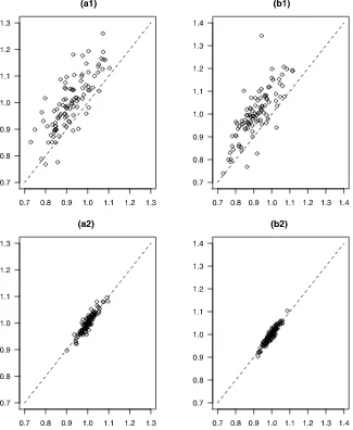
To visualize the accuracy of the posterior of SV, in Figure1 we plot the posterior means of SV components h1t and h2t against the generated values (averaged over t) for 100 simu-lated data samples, with T=100 and 1000, respectively. The posterior means ofh1tandh2tare the average over MCMC cy-cles and over time t. The figure shows that when the sample
sizeT=100, the posterior mean of SV is a fair estimate of the simulated SV, with a moderate upward bias. For a larger sample sizeT=1000, the average of the posterior mean becomes very close to the true SV.
To further examine the property of simulated SV, we plot the time series of true SV against the posterior of SV. We se-lect a random sample (by using the 100th sample) of gener-ated data with T =1000, and record the posterior of hjt for j=1, . . . ,4,t=1, . . . ,1000. To gain a better view, we plot in Figure2the middle portion of the time series (t=400 to 600) of the true SV [h1tin panel (a) andh4tin panel (b)], the poste-rior mean, and the posteposte-rior mean plus and minus 2 times sim-ulated posterior standard deviation bands (roughly 5 percentile to 95 percentile confidence bands for normally distributed ran-dom variables). The figure shows that the posterior of SV bands tracks the true SV quite well over time. In the figure, the stan-dard deviation of the posterior ofh1tdoes not shrink over time, which suggests that the resampling step of the particle filter suc-cessfully prevented degeneration. The deterministic conditional varianceh4tis estimated with high precision, the posterior stan-dard deviation is visually negligible compared to the variation of the conditional variance over time.
Next, to evaluate the performance of model selection, we further examine the posterior of model indices. Earlier we re-ported the posterior mean of the model index for selecting (B1,,A1,δ). One approach to selecting the best model is to include a variable when the posterior mean of the corresponding index is above a threshold. If we set such a threshold (say 0.9) in the above example for a large sample size(T=1000), then the true data generating model is selected. If the sample sizeT is much smaller then setting a high threshold may exclude too many variables. The threshold should be chosen judicially, de-pending on the sample size of the data.
An alternative criterion to the posterior mean of model index is the posterior mode, which corresponds to the most frequently visited model. If stochastic search is successful the most visited model is the data generating model. The number of parame-ters subject to stochastic search is 34, for a total number of 234 competing models. For 10,000 MCMC runs, the algorithm vis-its several hundred different submodels. For all data samples Table2summaries the average frequencies that the true model is visited. As the sample sizeTincreases, the frequency of visit-ing the true data-generatvisit-ing model for andB1increases. But the frequency of visiting the true SV model is not monotoni-cally increasing in the sample size in our experiment.
Note that the frequencies are averaged over 100 samples (the cross-sample standard deviations of the frequencies are re-ported in the parentheses.) So the averaged frequency of match-ing the whole data-generatmatch-ing model may be larger or smaller than the product of the averaged frequencies of matching each part of the model. Nonetheless, these numbers indicate that the stochastic search algorithm is highly effective in selecting the data generating model even with a modest sample size of T=100. WhenT =100, the true model is visited a remark-able 11.2% of the time. With a large sample sizeT=1000, the average odds of visiting the true model are overwhelming.
It is well known that an unrestricted model (setting all model indexes to unity) is often over-fitted and performs poorly in forecasting. We now compare the forecasting performance be-tween an unrestricted model and restricted models obtained
Figure 1. Posterior means and generated true values of sample average ofh1with (a1)T=100 and (a2)T=1000; andh2with (b1)T=100 and (b2)T=1000. The horizontal axis represents the generated SV and the vertical axis plots the corresponding posterior mean of SV, both are averaged over time for each of the 100 samples. The dashed line is the 45 degree line.
from stochastic search. We obtain Bayesian estimates under the unrestricted model and that through Bayesian stochastic search. We use the estimated parameters to make one-period-ahead forecast ofyj,T+1, for j=1, . . . ,4. We definey(j,trueT+)1=
bj0+Bj1xT+1, the prediction based onxT+1 and the jth row of the true parameters of (b0,B1). Lety(j,kT)+1 be the pre-diction based on the Gibbs output of the parameters at cy-cle k, ((k),b(k),a0(k),β(k), A(1k),δ(k),γ(bk), γψ(k), γ(ak), γ(δk), q(k),(k)). In fact,yj(,kT)+1 depends explicitly only onb(k) and is given byy(j,kT)+1=b(j0k)+B(j1k)xT+1.We define the prediction squared errors to be
1 K
K
k=1
y(j,trueT+)1−y(j,kT)+12, (47)
which depends only on the estimation errors of the parameters. We average over all MCMC cycles through stochastic search. This is an alternative to a typical Bayesian model averaging (BMA) (see, e.g.,Hoeting et al. 1999). In BMA ofNcompeting
models, posteriors of parameters would have to be simulated for each of theN models and the predicted value would then be weighted by the posterior ofNmodel probabilities. For the example above whenp=4,N=234. Clearly, it is impossible to compute all these competing models. An advantage of sto-chastic search in the article is to draw parameters conditioning on visited models. The frequently visited models are weighted heavily automatically. In contrast to the multiple models visited in stochastic search, the unrestricted model space consists of a single fixed model.
There are other methods besides BMA in the literature of forecasting. For example,Breiman(1996) has proposed an ap-proach named bagging by averaging predictions based on esti-mates derived from bootstrapped data. It has been shown to im-prove forecasting in macroeconomics. For example,Inoue and Kilian(2008) show that for forecasting consumer price inflation using 30 macroeconomic indicators, bagging performs better than equal weighted averaging of all prediction models based on each indicator and does equally well as BMA. Although both stochastic search and bagging can be used for model se-lection, there are several important differences. One advantage
Figure 2. h1t[in panel (a)] andh4t[in panel (b)] for one sample,t=400, . . . ,600. Solid=trueht, dashed=posterior mean ofht, dotted=
posterior mean+2 times standard posterior deviation ofht, dot-dashed=posterior mean−2 times standard posterior deviation ofht.
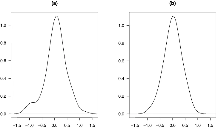
of stochastic search is that the resultant model restrictions may have economic interpretations while the averaged prediction from bagging is often ad hoc and does not correspond to an economic model. In addition, bagging is suitable for forecast-ing a scalar variable with a large number of exogenous predic-tors.Inoue and Kilian(2008) include lags of inflation in their model and limited bagging to exogenous predictors. The pres-ence of SV further complicates bootstrapping of serially cor-related data. Hence, for restricting a VAR with SV, stochastic search is much more convenient. Of course, it is interesting to compare the performance of alternative approaches to forecast-ing besides stochastic search. We will explore this in the future. Table 3 compares the prediction errors (47) averaged over 100 data samples for the restricted (stochastic search) model with those for the unrestricted models. The average prediction errors of the restricted model are about 30% smaller than the un-restricted model whenT=100 and around 20% smaller when T =1000. As the sample size increases, the prediction error and the improvement by stochastic search decrease.Maheu and Liu (2009) show that the BMA improves the prediction per-formance of GARCH models. We find this to be true for SV models. In Figure3, we plot the frequentist densities of predic-tion errors of the posterior mean ofy4T+1, defined for a given sample as K1Kk=1y(4k,T)+1−y(4true,T+)1,forT=100, for restricted and unrestricted models. The density of unrestricted model in Figure 3(a) shows greater dispersion than that with restricted
model in Figure3(b). The figure agrees with the results reported in Table3.
As in Maheu and Liu (2009), we also compute the pre-dictive likelihood of one-step-ahead out-of-sample prediction L(yT+1|y1, . . . ,yT), after integrating out parameters (including SV) and models. This quantity measures overall predictive fit of the models to the dataset. The stochastic search also dominates in terms of predictive likelihood: WhenT=100 the predictive likelihood for one-step-ahead forecast averaged over all data samples is−5.371 for the unrestricted model and is−5.342 for stochastic search.
The online Appendix contains a brief discussion on the ro-bustness of the algorithm to the prior hyper-parameters and the number of observations.
4.3 Discussion on Alternative Approaches to Inference of SV
In the particle filter algorithm, a multinomial resampling adds noise that may distort the drawn filter density from the true density, especially at the tails. The auxiliary sampling im-portance resampling filter ofPitt and Shephard(1999b) refines the particle filter to produce a more accurate approximation of the true filter density. For the example at hand, we find that the refined resampling produces similar results as AlgorithmF.
We now briefly discuss three approaches as alternatives to the one proposed in this study for inference of SV: direct sampling
Table 2. Average frequency of visiting the true model (p=4) (cross-sample standard deviations in parentheses)
Parameter Entire model(B1,,A1,δ) B1 (A1,δ)
# of parameters 34 20 6 8
T=100 0.112 (0.089) 0.197 (0.136) 0.623 (0.244) 0.901 (0.003)
T=1000 0.598 (0.016) 0.718 (0.018) 0.937 (0.003) 0.889 (0.007)
Table 3. Comparison of squared prediction errors (47) based on stochastic search (SS) and those based on unrestricted model, averaged over 100 data samples
Model Pred. errory1 Pred. errory2 Pred. errory3 Pred. errory4
SS,T=100 0.1358 0.1419 0.1160 0.1160 No restriction,T=100 0.1814 0.2330 0.1803 0.1714 % improvement with SS 25.14% 39.10% 35.50% 32.3%
SS,T=1000 0.0166 0.0136 0.0107 0.0158 No restriction,T=1000 0.0201 0.0182 0.0131 0.0181 % improvement with SS 17.41% 25.27% 18.32% 12.71%
using the Gilks adaptive rejection sampler, Gaussian approxi-mation of SV model byKim, Shephard, and Chib(1998) (who also use particle filter for evaluation of likelihood), and rejec-tion sampling of element-wise volatilities through the filtered volatilities.
The direct sampling approach through Adaptive Rejection SamplerbyGilks and Wild(1992) is an alternative to the fil-ter approach when the posfil-terior of eachhjtconditional on other parameters is log-concave. In our example, the running time for the adaptive rejection method based on log-concavity is on average about half that of the particle filter algorithm. How-ever, the generated samples of stochastic volatilityfrom the the rejection method exhibit a strong serial correlation over the MCMC cycles. It takes more MCMC cycles to achieve a result similar to the particle filter algorithm. Pitt and Shep-hard (1999a) show that the convergence of a single-move sampling algorithm for hjt conditional on (b,,a0,β,A1,
δ,hj,t−1,hj,t+1;y)is very slow, especially when the SV has a strong correlation and the variance of the SV is approximately zero. We find that the particle-filter-based block-move algo-rithm is quite efficient for such cases. Figure2(b) shows that the estimated conditional variance is nearly identical to the ones that generated data, even when the number of burn-in cycles is
small, the SV has a large AR coefficient and a near zero vari-ance.
To increase the efficiency of the computation over the single-move rejection-based method,Kim, Shephard, and Chib(1998) andChib, Nardari, and Shephard (2002) approximate the SV model by a Gaussian-linear model and evaluate the marginal likelihood by using a particle filter. As pointed out by a referee, particle filters play different roles in our study from that inKim, Shephard, and Chib (1998) and Chib, Nardari, and Shephard (2002). In the latter studies, particle filters are used to compute predictive likelihoodf(yt+1|ht,Yt,θ)given the model parame-tersθ, where the posterior ofθis simulated from MCMC in a mixture Gaussian state-space model that approximates the orig-inal SV model. In our study, particle filters are used to simulate SV jointly with model parametersθ. This is made possible by doing backward smoothing following forward filtering.
The importance sampling particle filter described above in-volves sampling and weighted resampling of vector-wise par-ticles for every Gibbs cycle. Using the fact that the condi-tional distributions of(hjt|hj,t−1,θ)are independent acrossj= 1, . . . ,p, we modify the rejection sampling algorithm specified inKim, Shephard, and Chib(1998) for our multivariate model. Sampling the vectorhtat once is equivalent to sample from the
Figure 3. Smoothed cross sample distribution of one-step-ahead average prediction errors ofy4T+1produced by unrestricted and restricted models. The size of each sampleT=100. (a) The distribution of prediction errors of unrestricted model. (b) The distribution of prediction errors of restricted model obtained via stochastic search.
posterior ofhjtelement-wise. We find that the element-wise re-jection method takes longer time to complete a given number of cycles.
5. AN APPLICATION TO DAILY FOREIGN
EXCHANGE RATE DATA
Kim, Shephard, and Chib(1998) conduct Bayesian estima-tion on an univariate model of stochastic volatilities of the ex-change rates. We extend their analysis by exploring how the exchange rates are correlated and whether they are driven by stochastic volatility in a SV VAR model (with one lag).
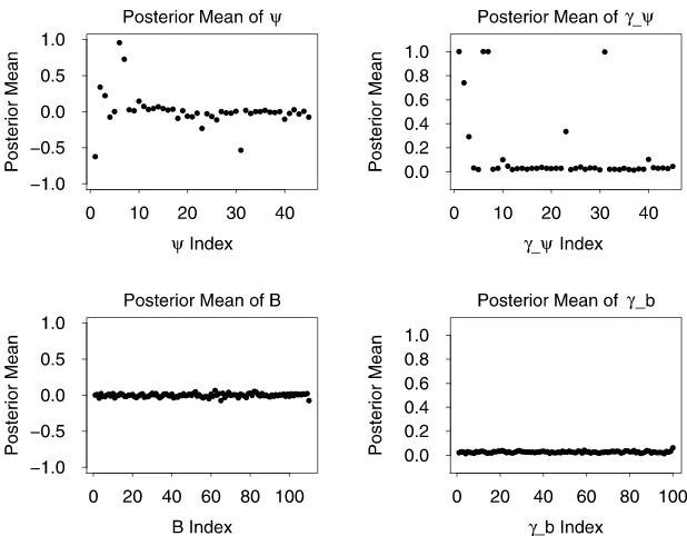
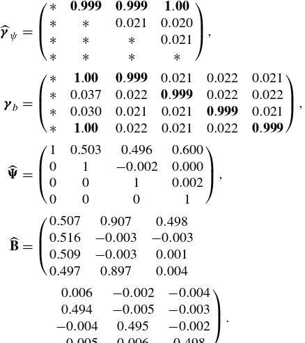
We examine the daily exchange rates of the U.S. dollar against the Euro, British Pound, Japanese Yen, Canadian Dol-lar, Mexican Peso, Brazilian Real, Switzerland Franc, Norwe-gian Krone, Singapore Dollar, and Indian Rupee (with this or-der in the VAR) between January 2001 and November 2005. The dataset are obtained from the Federal Reserve Bank of St Louis. To make our result comparable to that byKim, Shep-hard, and Chib (1998), we focus on the demeaned log dif-ferences of exchange rate as they do. Prior hyperparameters are the same as those in the numerical example, except the volatility prior parameters are set as s0=10−8, αq =0.1, and βq=0.05. We draw 50,000 MCMC cycles with 10,000 burn-in runs. Figure 4 is a scatter plot of the posterior mean of the nonredundant elements of [defined in (5)] and the corresponding model index γψ. The plot of andγψ sug-gests a strong correlation among the exchange rates. Figure4 also plots the posterior mean of regression coefficient matrix B=(b0,B1) and the model index of B1, γb. All the ele-ments of Bandγb are close to zero. The figure supports the restriction imposed by Kim, Shephard, and Chib (1998) that daily exchange rate returns are serially uncorrelated. Without imposing the restriction a priori as they do, we start from a
more general VAR model and arrive at the same conclusion via model selection. The posterior mean of the stochastic volatility and that of the corresponding model selection index areδ= (0.0002, 0.0010, 0.0147, 0.0018, 0.0129, 0.1693, 0.0158, 0.0068, 0.0141, 0.0089)′, γ
δ = (0.8930, 1.0000, 1.0000, 1.0000,1.0000,1.0000,1.0000,1.0000,0.9780,1.0000)′. Al-though the posterior mean of the SV parameter vectorδis small in magnitude, all elements ofδare selected at high frequencies. We conclude that the daily returns of exchange rates of dollar against major foreign currencies are serially uncorrelated and contemporaneously correlated, and that their conditional vari-ances are stochastic.
6. DISCUSSION
In this study we develop and implement an algorithm for Bayesian model selection of multivariate stochastic volatility models. We extend the stochastic search method ofGeorge and McCulloch(1993) for linear regression, andGeorge, Sun, and Ni(2008) for multivariate time series with fixed covariances. Our method applies to time varying covariances and provides a computationally feasible algorithm to select among a large number of competing models. Our simulation studies show that the particle filter-smoothing algorithm is effective for a small scale model with a moderately large sample size. We find that restricted models obtained through stochastic search outper-form unrestricted models in out-of-sample forecasts.
A number of generalizations are possible. First, a noninde-pendent setup of the Bernoulli hyper priors would allow great flexibility. Second, the model can be extended to allow jumps and/or non-Gaussian errors with heavy tails (seeChib, Nardari, and Shephard 2006). Finally, the modified Cholesky decompo-sition used in the article enjoy advantages such as computa-tional feasibility and easy statistical interpretability of the para-meters, but other parameterizations could be considered [e.g.,
Figure 4. Stochastic search of SV VAR(1) using daily exchange rate data: posterior means for,γψ,B, andγb. The matrices are vectorized by row.
those by Chiu, Leonard, and Tsui (1996) or Chen and Dun-son(2003)]. A comparison of different decompositions in mul-tivariate stochastic volatility models may lead to interesting fu-ture developments.
ACKNOWLEDGMENTS
Ni’s research was supported by a grant from the MU Re-search Council and by Hong Kong ReRe-search Grant Council grant CUHK4128/03H. Sun’s research was supported by the National Science Foundation grant SES-0720229, and NIH grants R01-MH071418 and R01-CA112159.
[Received August 2008. Revised October 2009.]
REFERENCES
Aguilar, O., and West, M. (2000), “Bayesian Dynamic Factor Models and Port-folio Allocation,”Journal of Business & Economic Statistics, 18 (3), 338– 357. [342]
Bauens, L., Laurent, S., and Rombouts, J. V. K. (2004), “Multivariate GARCH Models: A Survey,” discussion paper, CORE. [342]
Black, F., and Scholes, M. (1973), “The Pricing of Option and Corporate Lia-bilities,”Journal of Political Economy, 81, 637–659. [343]
Bollerslev, T., Chou, R. Y., and Kroner, K. F. (1992), “ARCH Modeling in Fi-nance. A Review of the Theory and Empirical Evidence,”Journal of Econo-metrics, 52, 5–59. [342]
Boscher, H., Fronk, E.-M., and Pigeot, I. (2000), “Forecasting Interest Rates Volatilities by GARCH(1,1)and Stochastic Volatility Models,”Statistical Papers, 41 (4), 409–422. [342,343]
Breiman, L. (1996), “Bagging Predictors,”Machine Learning, 24, 123–140. [351]
Carter, C. K., and Kohn, R. (1994), “On Gibbs Sampling for State Space Mod-els,”Biometrika, 81, 541–553. [348]
(1996), “Markov Chain Monte Carlo in Conditionally Gaussian State Space Models,”Biometrika, 83, 589–601. [348]
Chen, Z., and Dunson, D. B. (2003), “Random Effects Selection in Linear Mixed Models,”Biometrics, 59 (4), 762–769. [355]
Chib, S., Nardari, F., and Shephard, N. (2002), “Markov Chain Monte Carlo Methods for Stochastic Volatility Models,”Journal of Econometrics, 108, 281–316. [342,343,348,353]
(2006), “Analysis of High Dimensional Multivariate Stochastic Volatility Models,”Journal of Econometrics, 134, 341–371. [343,348,354] Chiu, T. Y. M., Leonard, T., and Tsui, K.-W. (1996), “The Matrix-Logarithmic Covariance Model,”Journal of the American Statistical Association, 91, 198–210. [355]
Christensen, B., and Kiefer, N. M. (2000), “Anticipated and Unanticipated Sto-chastic Volatility in Empirical Option Pricing,” working paper, Department of Economics, Cornell University. [343]
George, E. I., and McCulloch, R. E. (1993), “Variable Selection via Gibbs Sampling,”Journal of the American Statistical Association, 88, 881–889. [343,345,349,354]
George, E., Sun, D., and Ni, S. (2008), “Stochastic Search Model Selection for Restricted VAR Models,”Journal of Econometrics, 142, 553–580. [343, 345,354]
Gilks, W. R., and Wild, P. (1992), “Adaptive Rejection Sampling for Gibbs Sampling,”Applied Statistics, 41, 337–348. [353]
Hoeting, J. A., Madigan, D., Raftery, A. E., and Volinsky, C. T. (1999), “Bayesian Model Averaging: A Tutorial” (with discussion),Statistical Sci-ence, 14 (4), 382–417. [351]
Hol, E., and Koopman, S. J. (2002), “Stock Index Volatility Forecasting With High Frequency Data,” discussion paper, Tinbergen Institute. [342,343] Hull, J., and White, A. (1987), “The Pricing of Option on Assets With
Stochas-tic Volatilities,”Journal of Finance, 42, 281–300. [343]
Inoue, A., and Kilian, L. (2008), “How Useful Is Bagging in Forecasting Eco-nomic Time Series? A Case Study of U.S. Consumer Price Inflation,” Jour-nal of the American Statistical Association, 103, 511–522. [351,352] Jacquier, E., Polson, N. G., and Rossi, P. E. (1994), “Bayesian Analysis of
Sto-chastic Volatility Models” (with discussion),Journal of Business & Eco-nomic Statistics, 12, 371–417. [342]
(2002), “Bayesian Analysis of Stochastic Volatility Models,”Journal of Business & Economic Statistics, 20, 69–87. [343]
Justiniano, A., and Primiceri, G. E. (2008), “The Time Varying Volatility of Macroeconomic Fluctuations,”American Economic Review, 98, 604–641. [343]
Kim, H., Sun, D., and Tsutakawa, R. K. (2002), “Lognormal vs. Gamma: Extra Variations,”Biometrical Journal, 44 (3), 305–323. [345]
Kim, S., Shephard, N., and Chib, S. (1998), “Stochastic Volatility: Likelihood Inference and Comparison With Arch Models,”Review of Economic Stud-ies, 65, 361–394. [345,353,354]
Maheu, J. M., and Liu, C. (2009), “Forecasting Realized Volatility: A Bayesian Model Averaging Approach,”Journal of Applied Econometrics, 24, 709– 733. [352]
Melino, A., and Turnbull, S. M. (1990), “Pricing Foreign Currency Options With Stochastic Volatility,”Journal of Econometrics, 45, 239–265. [343] Pitt, M. K., and Shephard, N. (1999a), “Analytic Convergence Rates and
Para-meterization Issues for the Gibbs Sampler Applied to State Space Models,”
Journal of Time Series Analysis, 20, 63–85. [353]
(1999b), “Filtering via Simulation: Auxiliary Particle Filters,”Journal of the American Statistical Association, 94, 590–599. [352]
Shephard, N. G. (1996), “Statistical Aspects of ARCH and Stochastic Volatil-ity,” inTime Series Models in Econometrics, Finance and Other Fields. Monographs on Statistics and Applied Probability, Vol. 65, eds. D. R. Cox, D. V. Hinkley, and O. E. Barndorff-Nielsen, London: Chapman & Hall, pp. 1–67. [342]
Tauchen, G. (2005), “Stochastic Volatility in General Equilibrium,” working paper, Department of Economics, Duke University. [343]
Taylor, S. (1994), “Modeling Stochastic Volatility: A Review and Comparative Study,”Mathematical Finance, 4, 183–204. [342]
Uhlig, H. (1997), “Bayesian Vector Autoregressions With Stochastic Volatility,”
Econometrica, 65, 59–73. [347]
![Figure 2. hposterior mean1t [in panel (a)] and h4t [in panel (b)] for one sample, t = 400,...,600](https://thumb-ap.123doks.com/thumbv2/123dok/1149041.765529/12.594.109.471.47.274/figure-hposterior-mean-t-panel-h-panel-sample.webp)