07350015%2E2014%2E982755

(1)

Full Terms & Conditions of access and use can be found at

http://www.tandfonline.com/action/journalInformation?journalCode=ubes20

Download by: [Universitas Maritim Raja Ali Haji] Date: 11 January 2016, At: 18:49

Journal of Business & Economic Statistics

ISSN: 0735-0015 (Print) 1537-2707 (Online) Journal homepage: http://www.tandfonline.com/loi/ubes20

A Covariate Selection Criterion for Estimation of

Treatment Effects

Xun Lu

To cite this article: Xun Lu (2015) A Covariate Selection Criterion for Estimation of Treatment Effects, Journal of Business & Economic Statistics, 33:4, 506-522, DOI: 10.1080/07350015.2014.982755

To link to this article: http://dx.doi.org/10.1080/07350015.2014.982755

Accepted author version posted online: 20 Dec 2014.

Published online: 27 Oct 2015. Submit your article to this journal

Article views: 184

View related articles

(2)

A Covariate Selection Criterion for Estimation

of Treatment Effects

Xun LU

Department of Economics, Hong Kong University of Science and Technology, Kowloon, Hong Kong (xunlu@ust.hk₎

We study how to select or combine estimators of the average treatment effect (ATE) and the average treatment effect on the treated (ATT) in the presence of multiple sets of covariates. We consider two cases: (1) all sets of covariates satisfy the unconfoundedness assumption and (2) some sets of covariates violate the unconfoundedness assumption locally. For both cases, we propose a data-driven covariate selection criterion (CSC) to minimize the asymptotic mean squared errors (AMSEs). Based on our CSC, we propose new average estimators of ATE and ATT, which include the selected estimators based on a single set of covariates as a special case. We derive the asymptotic distributions of our new estimators and propose how to construct valid confidence intervals. Our Monte Carlo simulations show that in finite samples, our new average estimators achieve substantial efficiency gains over the estimators based on a single set of covariates. We apply our new estimators to study the impact of inherited control on firm performance.

KEY WORDS: Focused information criterion; Model averaging; Treatment effect; Unconfoundedness.

1. INTRODUCTION

One of the central questions in the semiparametric estimation of the average treatment effect (ATE) and the average treatment effect on the treated (ATT) is how to select proper covariates. Despite its importance, the literature on the selection of co-variates for estimating treatment effects is limited. Imbens and Wooldridge (2009, p. 50) pointed out that “a very important set of decisions in implementing all of the methods [of estimating treatment effects]. . .involves the choice of covariates,” but “the literature has not been very helpful,” and “it is clear that more work needs to be done in this area.”

In general, there are two important issues concerning the choice of covariates. First, the choice of covariates crucially de-pends on the unconfoundedness assumption. If this assumption is violated, the estimators of ATE and ATT would in general be inconsistent. In particular, Rosenbaum (1984), Heckman and Navarro-Lozano (2004), and Wooldridge (2005) warned that conditioning on too many covariates, especially those that are influenced by the treatment, can cause the unconfoundedness assumption to be violated easily. Chalak and White (2012) ex-amined how valid covariates should be chosen to satisfy the un-confoundedness assumption by invoking Reichenbach’s (1956) principle of common causes: if two variables are correlated, then either one causes the other or there is a common cause of both. Lu and White (2014, Sec.5) provided further discus-sions. Second, even if the unconfoundedness assumption is not a concern, using different sets of covariates may yield differ-ent estimation efficiencies (i.e., differdiffer-ent asymptotic variances). Hahn (2004) and White and Lu (2011) discussed this issue and show that it is not always desirable to condition on fewer or more covariates. The efficient choice of covariates depends on the underlying structures of potential outcomes, treatments and covariates. Intuitively, we should condition on the proxies of potential outcomes as much as possible, but on the proxies of treatments as little as possible. To analyze the underlying causal structures, we may use causal diagrams in the graph-ical model literature (see, e.g., Pearl 2009; VanderWeele and Shpitser 2011). All these results in the literature offer useful

insights into the choice of covariates. However, in practice, the details of the underlying causal structures are rarely known. The goal of this article is to provide a simple data-driven criterion to select or combine estimators of ATE and ATT in the presence of multiple candidate sets of covariates.

Specifically, the parameters we are interested in are ATE and ATT:

ATE₌E(Y(1)₋Y(0)) and ATT₌E(Y(1)₋Y(0)_|D₌1), whereDis a binary treatment andY(0) andY(1) are potential outcomes corresponding toD₌0 andD₌1, respectively. To estimate them, we often need to use covariates. In practice, researchers may face multiple sets of covariates. The natural criterion for deciding which set to use is the asymptotic mean squared errors (AMSEs) of the estimators of ATE and ATT. In this article, we provide estimators of the AMSEs, which are referred to as the covariate selection criterion (CSC). Based on the CSC, we can select the best estimator or combine all estimators optimally.

We consider two cases. First, we assume that all candidate sets of covariates are valid in the sense that conditioning on each set of covariates, the unconfoundedness assumption is satisfied, that is, (Y(0), Y(1)) and Dare independent conditioning on each set of covariates. Thus using any set of covariates leads to a consistent estimator. In this case, we have multiple con-sistent estimators. Our CSC is essentially the estimator of the asymptotic variance–covariance matrix. Based on the CSC, we propose a weighted average estimator that achieves the small-est asymptotic variance. This small-estimator is analogous to Lu and White’s (2014) feasible optimally combined GLS (FOGLeSs) estimator in the linear regression context.

Second, we allow some sets of covariates to be locally in-valid in the sense that the differences between the parameters of interest (i.e., ATE and ATT) and the parameters that can be

506

(3)

identified (i.e., those that are entirely based on the joint distribu-tion of the observable data) converge to zero at the rate of√n, wherenis the sample size. This could be because the difference between the distribution of (Y(0), Y(1)) conditioning on the co-variates andD₌1 and that conditioning on the covariates and D₌0 converges to zero at the rate of√n. Thus, for any given n,the unconfoundedness assumption is violated. However, at the limit whennapproaches infinity, the unconfoundedness sumption holds. This local asymptotic framework is often as-sumed in the model selection and model averaging literature (see, e.g., Claeskens and Hjort2008, CH hereafter). We show that by using the locally invalid covariates, the standardized es-timators of ATE and ATT converge in distribution to a nonzero mean normal distribution. Thus, the squared asymptotic bias is nonzero and of the same order as the asymptotic variance term. This local asymptotic approach essentially allows us to strike a balance between the bias and variance terms. Our CSC esti-mates both the bias term and the variance term. Based on our CSC, we propose a weighted average estimator that minimizes the AMSE. We show that the asymptotic distribution of the weighted average estimator is nonstandard (a nonlinear func-tion of a normal vector) and propose a simulafunc-tion-based method to construct confidence intervals.

If the unconfoundedness assumption is violated globally in the sense that the differences between the parameters of interest and the parameters identified are nonzero constants that do not change with the sample size, then the bias term dominates the variance term. Thus, theoretically speaking, we should never use globally invalid covariates. But even so, in the simulations, we apply our CSC to globally invalid covariates and find that our new average estimators perform reasonably well.

This article is related to the model averaging literature. Broadly speaking, this literature can be classified into the Bayesian model averaging (BMA) stream and the frequentist model averaging (FMA) stream. BMA has a long history (see, e.g., Hoeting et al. 1999 for a review), whereas FMA has a relatively short one. Claeskens and Hjort (2003), Hjort and Claeskens (2003), and CH provided detailed discussions on FMA and proposed a focused information criterion (FIC) that is similar to our CSC. Model averaging is mainly applied to estimate conditional means or conditional quantiles. Hansen (2007) and Hansen and Racine (2012) proposed Mallows’ crite-rion and a jackknife method for averaging linear regressions, re-spectively. Liu (2015) derived the asymptotic distribution of the average estimator in the local asymptotic framework for linear regressions. Chen, Jacho-Ch´avez, and Linton (2015) considered an averaging GMM estimator with an increasing number of mo-ment condition. Lu and Su (2015) proposed a jackknife method for averaging quantile regressions. DiTraglia (2012) applied the model averaging idea to the selection of instrument variables and proposes a focused moment selection criterion (FMSC).

In the context of estimation of treatment effects, recently, sev-eral papers have discussed the model selection or covariate se-lection. Vansteelandt, Bekaert, and Claeskens (2010) proposed a focused information criterion for covariate selection for estima-tion of the marginal causal odds ratio. De Luna, Waernbaum, and Richardson (2011) characterized a minimal subset that satisfies the unconfoundedness assumption from the original reservoir of covariates. Crainiceanu, Dominici, and Parmigiani (2008) pro-posed a two-stage statistical approach that takes into account the

uncertainty of covariate selection. There are also an increasing number of papers that apply the model averaging techniques to the estimation of treatment effects. Wang, Parmigiani, and Dominici (2012, WPD hereafter) developed a model averag-ing method called Bayesian adjustment for confoundaverag-ing (BAC) that jointly considers the treatment assignment and outcome models. Zigler and Dominici (2014, ZD hereafter) proposed a novel Bayesian model averaging method based on the likelihood that simultaneously considers the propensity score and outcome models. Our article differs from these papers in several aspects. First, WPD and ZD’s averaging methods are mainly Bayesian, while ours is frequentist. Second, we work in a local asymptotic framework that allows the unconfoundedness assumption to be violated locally, while WPD and ZD assumed that the largest set of covariates satisfies the unconfoundedness assumption, but some covariates may be redundant. Kitagawa and Muris (2013, KM hereafter) recently proposed a model averaging method for the propensity score weighting estimator for estimation of ATT in a local asymptotic framework. There are several differ-ences between KM and our article. First, KM’s model averaging method is based on the Bayes optimal weights with respect to the prior for the local parameters, while ours is “plug-in” -type frequentist model averaging as in CH. Second, we do not con-sider the specification of the functional form of the regression function or propensity score function, as they are nonparametri-cally estimated. For the tuning parameter in the nonparametric estimation, we simply use a “rule of thumb.” KM assumed that the largest (parametric) model of the propensity score is cor-rectly specified and discussed both the choice of covariates and the specification of the propensity score function. Third, their method focuses on a particular estimator of ATT, while ours can be applied to any estimators of ATE and ATT in the presence of multiple sets of covariates.

This article is organized as follows. In Section2, we discuss individual estimators for given sets of covariates. In Section3, we propose the CSC and average estimators when all sets of co-variates are valid. In Section4, we allow some sets of covariates to be locally invalid and propose the corresponding CSC and average estimators. In Section5, we propose a Hausman-type test to test for the unconfoundedness assumption. In Section 6, we conduct Monte Carlo simulations to demonstrate the su-perior performance of our new average estimators. In Section 7, we apply our new methods to study the effects of inherited family control on firm performance. Section8 concludes. All mathematical proofs are gathered in the appendix.

2. INDIVIDUAL ESTIMATORS

Consider a binary treatment Di and potential outcomes of

interestYi(0) andYi(1), corresponding to the possibilitiesDi =

0 andDi=1, respectively. The effects of interest are ATE:β0≡

E_[Yi(1)−Yi(0)] and ATT: γ0≡E[Yi(1)−Yi(0)|Di =1].

We consider J potential sets of covariates X1i,X2i, . . . , and

XJ i, whereXj i(j =1, . . . , J) is a vector of dimensionkj.We

do not impose any restrictions on theJsets of covariates. For example,kj’s can be different, that is, the dimensions ofXj i’s

can be different.Xj i’s can have common or distinct elements

and can be nested or nonnested. To construct the candidate sets of covariates, we often need to apply domain knowledge and use a priori information. The outcome we observe isYi =

(4)

DiYi(1)+(1−Di)Yi(0).We assume the data are independent

and identically distributed (iid).

Assumption A.1. We observe an iid sample: {Yi, Di,

X1i,X2i, . . . ,XJ i}, i=1, . . . , n.

Since we consider an iid sample, for notational simplicity, we suppress the subscriptias long as there is no confusion. Given each set of covariatesXj,we define

βj ≡E

We also define the propensity score as pj

are the parameters that can be identified in the sense that they can be represented entirely in terms of the joint distribution of the observable data. In general,βj =β0andγj =γ0.However,

they are both equal under the key unconfoundedness assump-tion: conditional on the covariatesXj, (Y(0), Y(1)) andDare

independent. In this section, we consider the estimators ofβj

andγjfor theJsets of covariates. Note that we do not make the

key unconfoundedness assumption in this section.

There are several estimators ofβj andγj in the literature.

As our CSC is not restricted to any particular estimator, we describe two common ones. These two estimators are efficient in the sense that they both achieve their semiparametric efficiency bounds for the given set of covariatesXj.Let ˆβj and ˆγj denote

the estimators ofβj andγj,respectively. Imbens, Newey, and

Ridder (2007) modified Hahn’s (1998) estimators and proposed the following imputation estimators:

ˆ

andm0j(.),respectively. They can be kernel-based Nadaraya–

Watson (NW) estimators or sieve-based estimators (see, e.g., Li and Racine2007). Hirano, Imbens, and Ridder (2003, HIR) proposed the following propensity score weighted (PSW) esti-mators:

A.2 is a high-level assumption requiring bothβˆandγˆ to be asymptotically normal with the influence functionsψi andφi,

respectively, that is,

.A.2 can be satisfied under primitive condi-tions. Hahn (1998), HIR, and Imbens, Newey, and Ridder (2007) discussed those primitive conditions on their estimators. To save space, we omit the details. For both the imputation estimators and PSW estimators,ψiandφi take the following forms:

ψj i=

Accordingly,VβandVγ are estimated as

ˆ

andVγ,respectively.

(5)

For a givenXj, it is desirable to use efficient estimators, such

as the imputation estimators and the PSW estimators. However, our CSC also allows inefficient estimators to be used as long as they are asymptotically normal with the convergence rate of √

n.

3. CSC FOR VALID COVARIATES

In this section, we provide a CSC for the simple case where all the candidate sets of covariates satisfy the unconfoundedness assumption. Following Dawid (1979), we use X ⊥Y|Z to denote the independence ofX andYgivenZ.

Assumption A.3. (i)D_⊥(Y0, Y1)|Xj and (ii) 0< p

A.3(i) requires that conditioning on each set of covariates, the key unconfoundedness assumption holds. It is certainly a strong assumption and we will relax it in the next section. Lu and White (2014, sec.5) discussed how to find multiple sets of valid candidate covariates that satisfy A.3(i).

A.3(ii) is the overlap assumption that is commonly made in the treatment effect literature. Note that if {Xj}J_j₌1 is nested

such thatX1⊆X2· · · ⊆XJ,we only require 0< p(XJ)<1,

which implies A.3(ii) by the law of iterated expectations. If the overlap assumption does not hold, the asymptotic variance terms,VβandVγ,can be infinite, as shown in Khan and Tamer

(2010). Crump et al. (2009) develop a systematic method to address the lack of overlap by focusing on a subpopulation. In principle, if A.3(ii) is violated, we can also apply our methods to a proper subpopulation. For simplicity, however, we maintain this overlap assumption.

Given that we haveJsets of covariates that satisfy the un-confoundedness assumption, we haveJconsistent estimators of β0 andγ0.Hence, we want to select the optimal estimator or

combine all estimators optimally. Let w₌(w1, w2, . . . , wJ)′

be aJ_×1 weight vector such thatJj=1wj =1.We propose

the following average estimators ofβ0andγ0:

ˆ

We can impose various restrictions onw.For example, if we allow only one element ofwto be 1 and set the other elements to 0, then we are selecting a single estimator. Therefore, the single best estimator is a special case of the average estimator. Another common restriction is that the weights are all positive, that is, 0≤wj ≤1. This restriction is often imposed in the

model averaging literature (see, e.g., Hansen2007; Hansen and Racine2012).

To obtain ˆβ(w) and ˆγ(w),the key step is to determine the weightw.We choose a weightwthat minimizes the AMSEs. It is easy to see that

√

Thus, in this case

AMSEβ(w)=w′Vβwand AMSEγ(w)=w′Vγw.

We propose the following CSC forβ0andγ0:

CSCβ(w)=w′Vˆβw and CSCγ (w)=w′Vˆγw.

If we do not impose any restrictions onwother thanJj=1wj =

1, it is easy to show that the estimated optimal weights are ˆ whereIis theJ_×1 vector of ones. Thus, the average estimators ofβ0andγ0are respectively,

and the average estimators satisfy √

γ∗_{based on the asymptotic results above directly. Our average}

estimators ˆβ∗_{and ˆ}_γ∗_{are similar to the FOGLeSs estimators}

pro-posed by Lu and White (2014). They considered combining es-timators for core regression coefficients in the linear regression context, whereas here we consider averaging semiparametric estimators of ATE and ATT.

Remark 1. In this simple case, to select the single best esti-mator amongβˆ (orγˆ),we can simply choose thejth element ofβˆ(orγˆ),such that thejth diagonal element of ˆVβ (or ˆVγ) is

smallest.

Remark 2. To ensure the weights are all positive, we can minimize CSCβ(w) or CSCγ (w) with the restrictions that

J

j=1wj =1 and 0≤wj ≤1, j=1, . . . , J.This can be

im-plemented using quadratic programming in standard software such as Matlab.

Remark 3. An alternative way of averaging the estimators in the literature is to use smoothed averaging. Specifically, let

ˆ

Vβ,j and ˆVγ ,j be thejth diagonal element of ˆVβand ˆVγ,

respec-tively. Then the smoothed average estimators ofβ0andγ0 are

respectively

which can be calculated easily.

Remark 4. Here there is no natural ordering of{Xj}Jj=1,hence

we cannot order the estimators{βˆj}Jj=1and{γˆj}Jj=1 according

to their asymptotic variances easily. Even if{Xj}Jj=1 is nested

(6)

and thus ordered, ranking the estimators is complicated, as it is not always more efficient to condition on more covariates. As pointed out by Hahn (2004) and White and Lu (2011), some-times using a smaller set of covariates may result in a more efficient estimator. Whether a large or a small set of covari-ates should be used depends on the underlying structure of (D, Y(0), Y(1),X1, . . . ,XJ),which may be difficult to judge

in practice. For further discussion on this issue in the linear regression context, see Lu and White (2014).

Remark 5. Here we propose to combine estimators. One natu-ral question is whether we can combine covariates. For example, we could use the union of{Xj}Jj=1 as one set of covariates to

estimate β0 and γ0. However, this is not a good strategy for

two reasons. First, A.3 does not imply thatDand (Y0, Y1) are

independent conditioning on the union of{Xj}J_j₌1.It is easy to

find counter-examples. In fact, Heckman and Navarro-Lozano (2004) and Wooldridge (2005) explicitly warned that condition-ing on a large set of covariates, the unconfoundedness assump-tion can be violated. Second, even if the unconfoundedness assumption is satisfied for the union of{Xj}Jj=1,the efficiency

of the estimators may suffer due to the use of a large set of covariates as discussed in Remark 4 above.

4. CSC FOR LOCALLY INVALID COVARIATES

In this section, we consider the case where some sets of candidate covariates violate the unconfoundedness assumption locally. We work on a local asymptotic framework, thus it is necessary to introduce a triangular array of the data.

Assumption A.1′_. _Let_{_D_i_{, Y}_i_,_X₁_ni_,_X₂_ni_{, . . . ,}_X_{J ni}_, ₁_≤_i_≤

n, n₌1,2, . . ._}be the a triangular array of random vectors and for a givenn,{Di, Yi,X1ni,X2ni, . . . ,XJ ni}, i =1, . . . , nare

iid.

We assume that the treatment Di, the potential outcomes

Yi(0) and Yi(1), and thus the observed outcome Yi do not

depend on the sample sizen.Thus the parameters of interestβ0

(ATE) andγ0(ATT) do not change withn.Define

βj n≡E

m1j n

Xj ni

−m0j n

Xj ni

and γj n≡E

m1j n

Xj ni

−m0j n

Xj ni

|Di =1

,

where

m1j n

Xj ni

=EYi |Di =1,Xj ni

and m0j n

Xj ni

=EYi |Di =0,Xj ni

.

For notational simplicity, we omit theiandnsubscripts as long as there is no confusion.

Assumption A.4. Suppose that there is a known integer J0

such that 1≤J0< J.

(i) Forj ₌1, . . . , J0, Di ⊥(Yi(0), Yi(1))|Xj ni.

(ii) Forj ₌J0+1, . . . , J,there exist unknown constantsδj

andλjthat do not depend onnsuch thatβj n =β0+

δj

√

n+

o(n−1/2_{) and}_γ

j n=γ0+

λj

√_n₊on−1/2_.

(iii) For j ₌1, . . . , J, 0< pj n(Xj ni)<1, where pj n(Xj ni)

=E₍Di|Xj ni).

A.4(i) requires at least one known set of covariates to be valid. This allows us to estimate the bias term of the estima-tors based on the locally invalid covariates. Note that there is no restriction on how to construct theJ0 sets of valid

co-variates. For example, one such set can be the union of all available covariates or a small subset containing the most rel-evant covariates. To determine such J0 sets of valid

covari-ates, unavoidably we need to make some subjective judgments using knowledge of the underlying structures. If all sets of covariates are (locally or globally) invalid, then none of the standardized individual estimators has an asymptotic distribu-tion centered at 0. This renders statistical inference impossible. Note that in the traditional way of estimating ATE and ATT using a single set of covariates, subjective judgment is also required.

Admittedly, the assumption that at least one set of covariates is known to be valid is the major limitation of our approach. However, assumptions like A.4(i) are often made in the model averaging literature. For example, DiTraglia (2012) assumed that there are enough known valid instruments to identify the parameter of interest in his average instrumental variable esti-mator. Similarly, CH and Liu (2015) assumed that the largest model is correctly specified, thus all the parameters are con-sistently estimated with zero asymptotic bias using the largest model. All these methods involve some subjective judgments, such as choosing valid instruments or a large model that is as-sumed to be correctly specified.

Though it is fine to use only theJ0 sets of valid covariates,

to reduce the AMSE even more, it is desirable to make further use of locally invalid covariates. A.4(ii) requires the remaining J₋J0sets of covariates to be locally invalid in the sense that

the differences between the parameters of interest (β0 andγ0)

and the parameters identified (βj nandγj n) converge to 0,as the

sample size approaches infinity. Thus in the limit, the uncon-foundedness assumption is satisfied. However, for a givenn,the unconfoundedness assumption is violated. To better understand A.4(ii), note that

βj n−β0=E[

EYi(0)|Di =1,Xj ni

−EYi(0)|Di =0,Xj ni

≡b1n(Xj ni)

|Di =1 ]·E(Di)

+E_[EYi(1)|Di=1,Xj ni

≡b0n(Xj ni)

|Di =0 ]·(1−E(Di))

γj n−γ0=E[

EYi(0)|Di=1,Xj ni

≡b1n(Xj ni)

|Di =1].

(7)

White and Chalak (2013) usedb1n sure the degrees of departure from the unconfoundedness for Yi(0) andYi(1) atXj ni, respectively.b1n

are both zero when the unconfoundedness assumption is sat-isfied. Essentially, here we requireb1n

converge to 0 at the rate of√n.One intuitive way of understand-ing condition A.4(ii) is to think of the locally invalid covariates as being generated as

⎛

J i are some random variables

satis-fying (Yi(0), Yi(1))⊥Di |X∗j i for j =J0+1, . . . , J and

x(J0+1)i, . . . , xJ iare some other random variables.

A.4(ii) does not literally mean that the real-world data are generated in this way. Instead, as a device, it ensures that the squared-bias term of the estimators is of the same order as the variance term (n−1₎_,_{which allows us to trade-off the bias and}

variance terms. This can be thought of as a mimic of the bivariance trade-off in finite samples. If the unconfoundedness as-sumption is violated globally in the sense that neither (βj n−β0)

norγj n−γ0

converges to zero asnapproaches infinity, then the bias term will dominate and the globally biased estimators should never be used. This “local asymptotic” approach is com-monly used in the model averaging literature (e.g., CH and Liu 2015), in the study of weak instrument variables (e.g., Staiger and Stock1997), and in the study of local alternatives in hy-pothesis testing in terms of Pitman drift. A.4(iii) is the overlap assumption discussed in Section3.

The next lemma shows the behavior of the individual estima-tors under A.4. random normal vector with mean zero and covariance– variance matrix Vβ and δ is a J×1 vector: δ= random normal vector with mean zero and covariance– variance matrix Vγ and λ is a J×1 vector: λ=

(0, . . . ,0, λJ0+1, . . . , λJ)′.

We consider the average estimators

ˆ

which include the selected single best estimator as a special case. It is easy to see that the AMSEs of ˆβ(w) and ˆγ(w) are,

Note thatVβ andVγ can be estimated consistently, but it turns

out that the bias termsδandλcannot. For simplicity, we assume thatJ0 =1,that is, only the first set of covariates is valid. For the

general case ofJ0>1,see Remark 8. Then the natural estimator

of the bias termδj, j =2, . . . , J,is ˆδj =√n

_ˆ βj −βˆ1

, that is, the estimator ofδis

ˆ

Similarly, the estimator ofλis ˆ

The next proposition describes the behavior of the bias estimators.

Proposition 2. Suppose that A.1′_,_{A.2, and A.4 hold. Then}

(i) δˆ_→d δ₊SP_∼Nδ, SVβS′

Proposition 2 states that the estimator of the bias termδˆ(or ˆ

λ) converges in distribution to a normal vector with the mean of δ(orλ). Thereforeδˆ(orλˆ) is not a consistent estimator ofδ(or λ). It is tempting to estimate AMSEβand AMSEγ respectively

by their sample analogues: w′δˆδˆ′₊Vˆβ

Similarly, the CSC forγ0is

CSCγ(w)=w′

definite. Thus the solution to the unconstrained minimization problem may not exist. To solve the problem, one simple way is to impose restrictions on the weights such as 0≤wj ≤1.

Thus, the optimal weights are defined as ˆ

The next proposition studies the properties of our CSC. Proposition 3. Suppose that A.1′_,_{A.2, and A.4 hold. Then}

(8)

(i) CSCβ(w)

Hence, our average estimators are defined as ˆ

β∗ ₌βˆwˆ_β∗₌wˆ∗′_ββˆand ˆγ∗₌γˆwˆ_γ∗₌wˆ∗′_γγ .ˆ The next proposition shows the asymptotic distribution of the average estimators.

√

The asymptotic distribution of ˆβ∗_{(or ˆ}_γ∗_{) is nonstandard and}

is a complicated nonlinear function of a normal vectorP(orQ), asw∗

β(orwγ∗) also depends onP(orQ). To obtain the confidence

interval, we propose to use the simulation-based method adopted in CH. For brevity, we only describe the method for ˆβ∗_. _The

method for ˆγ∗ _{is similar. For any given value of}_δ,_{we propose}

the following algorithm to obtain the 100(1−α)% confidence interval for ˆβ∗.

Algorithm 1 (Confidence interval ofβˆ∗for a givenδ). Simu-late a sufficiently large number (sayK) ofJ _×1 normal vectors P(k) confidence interval is constructed as

"

The algorithm is easy to implement given the value of δ. However, we do not know the value ofδ. One simple way to overcome this is to use the estimatedδ.ˆ The confidence interval is thus constructed as

" Alternatively, we can use the two-stage procedure proposed by CH (p. 210). To do so, we first need to construct the confi-dence regions of the estimators of the bias terms. Specifically, let ˜Sbe the known (J ₋1)×J matrix:

is easy to show that the Wald-statistic for testing the null that ˜ constructed by inverting the test statistic, that is,

ˆ

A_δ˜ =δ˜∗:F_δ˜δ˜∗≤χ_J2₋₁_,₁₋_τ, (8) whereχ2

J−1,1−τis the (1−τ)th quantile of theχ

2

J−1distribution.

We propose the following two-stage algorithm to obtain the confidence interval of ˆβ∗_.

Algorithm 2 (Two-stage confidence interval ofβˆ∗_).

Step 1: Find the 100 (1−τ) % confidence set ofδ˜: ˆAδ˜as in

Step 3: Construct the confidence interval as

"

The next proposition shows that the two-stage confidence interval has valid coverage properties.

lim

Proposition 5 establishes the validity of the two-stage con-fidence interval for ˆβ∗_{. However, there are two problems}

as-sociated with it. First, it can be conservative in the sense that the actual coverage can be larger than the nominal coverage. Second, the computation can be intensive, as it requires calcu-lating ˆaβ([0δ˜∗′]′) and ˆbβ([0δ˜∗′]′) for eachδ˜∗ in the confidence

region ˆA_δ˜. In the simulation, we show that the naive approach (Equation (6)) actually performs remarkably well in finite sam-ples. DiTraglia (2012) also reported the excellent performance of the naive approach in other contexts. The confidence inter-vals for ˆγ∗ can similarly be constructed. Other methods, such as those proposed in Zhang and Liang (2011), can also be used to construct the confidence intervals.

Remark 6. As discussed in Section3, the single best estima-tor ofβ0(γ0) is thejth element ofβˆ(γˆ) such that CSCβ(w(j))

(CSCγ(w(j))) is smallest, where w(j) is a J×1 selection

vector with the jth element being 1 and others 0. We can also construct the smoothed averaging estimators forβ0andγ0

(9)

Table 1. Relative efficiency: valid covariates

Valid

CSC Smoothed CSC

DGP n Set 1 Set 2 Set 3 Set 4 Set 5 average average selected

Average treatment effect (β0)

1 250 1.000 0.765 1.133 0.771 1.123 0.778 0.803 0.873

500 1.000 0.847 1.258 0.861 1.251 0.810 0.839 0.916

1000 1.000 0.922 1.362 0.930 1.377 0.840 0.868 0.946

5000 1.000 0.943 1.360 0.928 1.390 0.839 0.861 0.938

2 250 1.000 0.738 1.006 0.730 0.996 0.794 0.756 0.858

500 1.000 0.811 1.141 0.834 1.118 0.820 0.848 0.892

1000 1.000 0.878 1.218 0.887 1.213 0.836 0.906 0.914

5000 1.000 0.905 1.240 0.892 1.256 0.833 0.924 0.911

3 250 1.000 0.766 0.977 0.786 0.980 0.742 0.806 0.808

500 1.000 0.838 1.072 0.825 1.045 0.797 0.860 0.860

1000 1.000 0.886 1.112 0.884 1.114 0.821 0.878 0.881

5000 1.000 0.908 1.139 0.897 1.130 0.847 0.886 0.890

Average treatment effect on the treated (γ0)

1 250 1.000 0.614 0.994 0.619 0.983 0.650 0.679 0.733

500 1.000 0.748 1.175 0.756 1.139 0.730 0.764 0.819

1000 1.000 0.847 1.280 0.843 1.301 0.773 0.807 0.866

5000 1.000 0.843 1.282 0.828 1.319 0.755 0.776 0.831

2 250 1.000 0.560 0.853 0.554 0.837 0.615 0.590 0.648

500 1.000 0.663 1.006 0.680 0.967 0.692 0.700 0.724

1000 1.000 0.753 1.095 0.750 1.096 0.724 0.774 0.762

5000 1.000 0.786 1.127 0.770 1.143 0.732 0.800 0.782

3 250 1.000 0.737 0.978 0.753 0.970 0.757 0.801 0.803

500 1.000 0.818 1.080 0.803 1.042 0.830 0.870 0.872

1000 1.000 0.861 1.112 0.864 1.116 0.879 0.903 0.904

5000 1.000 0.868 1.143 0.854 1.149 0.841 0.878 0.879

NOTE: The numbers in the main entries are the MSEs standardized by the MSE of the estimator based on covariate set 1.

respectively as

J

j₌1

exp−12CSCβ(w(j))

J

k=1exp

−12CSCβ(w(k))

βˆj

and

J

j=1

exp−12CSCγ(w(j))

J

k=1exp

−12CSCγ(w(k))

γˆj.

The confidence intervals can also be constructed in the way that is similar to Algorithms 1 and 2.

Remark 7. The assumption of locally invalid covariates al-lows us to trade-off bias and variance terms. If some candidate sets of covariates are indeed globally invalid, then their corre-sponding elements in the CSC will be of ordernand much larger than those of locally invalid and valid sets of covariates. There-fore, in principle, to minimize the CSC, the optimal weights of the estimators based on the globally invalid covariates should be 0 in large samples. So, we can apply the same CSC to glob-ally invalid covariates. In the simulations, we consider globglob-ally invalid covariates and find that our average estimators perform reasonably well and sometimes even outperform the estimator based on valid covariates only.

Remark 8. For simplicity, when introducing the CSC for lo-cally invalid covariates, we assume that there is only one set of valid covariates. In practice, however, we may consider multiple sets of valid covariates. In this case, we can construct the CSC

average estimator in two steps. First, optimally combine the esti-mators based only on the sets of valid covariates as in Section3. Second, estimate the bias term using the average estimator in the first step and construct a similar CSC to combine all estimators. Below, we describe in detail the two steps for estimatingβ0. The

two-step procedure forγ0is similar. We use superscripts (1) and

(2) to denote the first-step and the second-step, respectively. Step 1: Let βˆ(1)_≡( ˆβ1,βˆ2, . . . ,βˆJ0) be the estimators ofβ0

using theJ0sets of valid covariatesX1,X2, . . . ,XJ0.

Fur-ther, let ˆV_β(1) be the estimator of the variance-covariance matrix ofβˆ(1)_{. Let ˆ}_w∗(1)

β ≡( ˆw

∗(1)

β,1, . . . ,wˆ

∗(1)

β,J0) be the

opti-mal weights in the first step for estimating β0. Then, as

shown in Section3,

ˆ w_β∗(1)₌

I(1)′_Vˆ(1)

β

−1

I(1)

−1

I(1)′_Vˆ(1)

β

−1

,

whereI(1)_{is the}_J

0×1 vector of ones. The corresponding

optimal average estimator ofβ0is ˆβ∗(1)=wˆβ∗(1)′βˆ(1).

Step 2: Letδˆ(2)

≡(0, . . . ,0,δˆ(2)_J

0+1, . . . ,δˆ

(2)

J )′denote the

esti-mator of the bias termδ_≡(0, . . . ,0, δJ0+1, . . . , δJ)′in the

second step. We can estimate the bias term based on the first-step estimator ˆβ∗(1)_. _{That is, ˆ}_δ(2)

j =

√

n( ˆβj −βˆ∗(1)),

j ₌J0+1, . . . , J.Then,δˆ(2)can be written succinctly as

ˆ

δ(2) ₌√nSˆβ·β,ˆ (9)

(10)

Table 2-1. Relative efficiency: locally invalid covariates—Case 1

Valid Locally invalid

CSC Smoothed CSC

DGP n Set 1 Set 2 Set3 Set 4 Set 5 average average selected

1 250 1.000 0.765 1.133 0.933 1.626 0.818 0.850 0.885

500 1.000 0.847 1.258 1.085 1.982 0.874 0.888 0.922

1000 1.000 0.922 1.362 1.170 2.194 0.904 0.919 0.952

5000 1.000 0.943 1.360 1.219 2.432 0.922 0.935 0.972

2 250 1.000 0.738 1.006 0.783 1.226 0.800 0.745 0.863

500 1.000 0.811 1.141 0.931 1.502 0.845 0.857 0.881

1000 1.000 0.878 1.218 0.994 1.664 0.873 0.909 0.922

5000 1.000 0.905 1.240 1.057 1.893 0.896 0.946 0.926

3 250 1.000 0.766 0.977 0.924 1.206 0.769 0.822 0.823

500 1.000 0.838 1.072 0.976 1.320 0.843 0.881 0.882

1000 1.000 0.886 1.112 1.027 1.392 0.856 0.886 0.888

5000 1.000 0.908 1.139 1.046 1.482 0.891 0.911 0.912

1 250 1.000 0.614 0.994 0.746 1.302 0.689 0.723 0.745

500 1.000 0.748 1.175 0.910 1.557 0.786 0.803 0.821

1000 1.000 0.847 1.280 0.995 1.735 0.831 0.855 0.883

5000 1.000 0.843 1.282 0.986 1.851 0.829 0.844 0.862

2 250 1.000 0.560 0.853 0.602 0.978 0.633 0.600 0.671

500 1.000 0.663 1.006 0.735 1.146 0.704 0.706 0.728

1000 1.000 0.753 1.095 0.818 1.332 0.755 0.778 0.785

5000 1.000 0.786 1.127 0.868 1.508 0.778 0.816 0.805

3 250 1.000 0.737 0.978 0.928 1.229 0.762 0.809 0.810

500 1.000 0.818 1.080 0.957 1.285 0.841 0.880 0.881

1000 1.000 0.861 1.112 0.991 1.310 0.867 0.894 0.895

5000 1.000 0.868 1.143 0.940 1.299 0.865 0.889 0.890

NOTE: See the note toTable 1.

where ˆSβis aJ×Jmatrix:

ˆ Sβ ≡

⎡ ⎢ ⎢ ⎢ ⎢ ⎢ ⎢ ⎣

0 0 ... 0 0 ... 0

...

0 0 ... 0 0 ... 0

−wˆ∗_β,(1)₁ ₋wˆ_β,∗(1)₂ ... ₋wˆ∗_β,J(1)

0 1 ... 0

...

−wˆ∗_β,(1)₁ ₋wˆ_β,∗(1)₂ ... ₋wˆ∗_β,J(1)

0 0 ... 1

⎤ ⎥ ⎥ ⎥ ⎥ ⎥ ⎥ ⎦ .

Then the CSC in the second step for estimatingβ0is

CSC(2)β (w)=w′

n_·Sˆββˆβˆ′Sˆβ′ −SˆβVˆβSˆβ′ +Vˆβ

w.

Hence the corresponding optimal weights in the second step are ˆw_β∗(2)₌arg minw∈WCSC

(2)

β (w) and the eventual

estimator ofβ0is ˆβ∗(2)=wˆβ∗(2)′βˆ.

The theoretical property of ˆβ∗(2)

is similar to that in the case withJ0=1,given that the weights ˆw∗

(1)

β are consistent

esti-mators of the optimal weights that minimize the AMSE of the average estimator based on theJ0sets of valid covariates in the

first step. The confidence interval of the two-step ˆβ∗(2)can also be constructed following Algorithms 1 and 2 with minor mod-ifications. For example, for the simple method of Algorithm 1, the only difference is that in Equation (6), we replaceδˆwithδˆ(2)

defined in Equation (9). In Algorithm 2, we use the confidence set ofδˆ(2)_{instead of that of}_δ._ˆ

5. A HAUSMAN-TYPE TEST

We have provided two CSC. One requires all sets of covariate to be valid, while the other allows some sets to be locally invalid. In practice, we need to decide which CSC to use. We may use some domain knowledge to determine whether the unconfound-edness assumption is plausible (see, e.g., Lu and White2014). Alternatively, we may test the null hypotheses

Hypothesis 1:H₁₀_:β1=β2= · · · =βJ

and Hypothesis 2:H₂₀_:γ1=γ2= · · · =γJ.

We can construct a Hausman-type test for these two hy-potheses. Below, we focus on Hypothesis 1, as the test for Hypothesis 2 is similar. Let ˜S be as defined in Equation (7). Hypothesis 1 is equivalent to ˜Sβ ₌0. The Wald-test statistic is just

Wβ=n·βˆ′S˜′

_˜ SVˆβS˜′

−1

˜ Sβˆ.

The next proposition describes the behavior of the test statistic under the null, the global alternatives and the local alternatives. The global and local alternatives for ATE are defined respec-tively as

H₁_A:H₁₀is false andH₁_a :βj =β1+

δj

√_n

forj ₌2, . . . , J and at least oneδj =0.

(11)

Table 2-2. Relative efficiency: locally invalid covariates—Case 2

Valid Locally invalid

CSC Smoothed CSC

1 250 1.000 0.936 1.626 0.933 1.626 0.934 0.981 0.993

500 1.000 1.077 1.975 1.085 1.982 0.975 1.008 1.024

1000 1.000 1.163 2.195 1.170 2.194 0.988 1.019 1.032

5000 1.000 1.219 2.413 1.219 2.432 0.997 1.030 1.045

2 250 1.000 0.794 1.238 0.783 1.226 0.902 0.809 0.958

500 1.000 0.914 1.527 0.931 1.502 0.935 0.945 0.982

1000 1.000 0.985 1.673 0.994 1.664 0.945 1.003 0.976

5000 1.000 1.060 1.892 1.057 1.893 0.967 1.075 1.003

3 250 1.000 0.905 1.204 0.924 1.206 0.899 0.952 0.952

500 1.000 0.992 1.327 0.976 1.320 0.935 0.984 0.985

1000 1.000 1.034 1.397 1.027 1.392 0.942 0.978 0.979

5000 1.000 1.053 1.481 1.046 1.482 0.964 1.007 1.007

1 250 1.000 0.744 1.287 0.746 1.302 0.876 0.934 0.944

500 1.000 0.907 1.595 0.910 1.557 0.914 0.958 0.971

1000 1.000 0.995 1.726 0.995 1.735 0.927 0.965 0.975

5000 1.000 0.993 1.821 0.986 1.851 0.927 0.972 0.983

2 250 1.000 0.613 0.982 0.602 0.978 0.829 0.700 0.911

500 1.000 0.721 1.195 0.735 1.146 0.855 0.775 0.914

1000 1.000 0.817 1.336 0.818 1.332 0.874 0.845 0.924

5000 1.000 0.877 1.506 0.868 1.508 0.892 0.898 0.937

3 250 1.000 0.903 1.238 0.928 1.229 0.894 0.936 0.936

500 1.000 0.977 1.309 0.957 1.285 0.934 0.961 0.962

1000 1.000 0.989 1.308 0.991 1.310 0.936 0.965 0.965

5000 1.000 0.953 1.287 0.940 1.299 0.927 0.953 0.953

Proposition 6.

(i) Suppose that A.1 and A.2 hold. Then underH₁₀,Wβ d

→

χ_J2₋₁.

(ii) Suppose that A.1 and A.2 hold. Then under H₁_A, P Wβ > en

→1,for any nonstochastic sequenceen=

o(n).

(iii) Suppose that A.1′ _{and A.2 hold. Then under} H₁_a, Wβ

d

→δ˜₊SP˜ _·SV˜ βS˜′

−1

·δ˜₊SP˜ ′, where δ˜₌ (δ2, . . . , δJ) andPis as defined in Lemma 1(i).

The same results hold for Hypothesis 2. One practical way to decide whether to use the CSC for valid covariates or the CSC for locally invalid covariates is to test Hypotheses 1 and 2 first. If the tests do not reject, we use the CSC for valid covariates. If they do, we use the CSC for locally invalid covariates. This procedure is practical and similar to that recommended by Lu and White (2014), although it may suffer from the well-known pretest problem.

Remark 9. The above testing procedure can also help to de-termineJ0 in the case whereJ0 might be larger than 1. For

example, suppose that the first set of covariates is valid and we are uncertain about the validity of the other sets of covari-ates. Then, we can test the hypotheses:β1=βj andγ1=γj for

j ₌2, . . . , J.If we fail to reject the hypotheses for thejth set of covariates, we treat it as valid. Otherwise, we treat it as invalid.

After determiningJ0>1 sets of valid covariates, we can follow

the two-step procedure described in Remark 8 to construct our CSC average estimator.

6. MONTE CARLO SIMULATIONS

We conduct Monte Carlo simulations to examine the finite sample performance of our method. We consider three cases: (1) all sets of covariates are valid, (2) some sets of covariates are locally invalid, and (3) some sets of covariates are globally invalid. For each case, we consider the following three data generating processes (DGPs):

DGP 1 : Y(0)=1+U+2ǫYandY(1)=2+U+2ǫY, DGP 2 : Y(0)₌(1₊U+2ǫY) andY(1)=(2+U+2ǫY), DGP 3 : Y(0)=(1+U+2ǫY)2 andY(1)=(2+U+2ǫY)2, whereis the standard normal CDF,D₌1_{X∗₊₂_ǫ_D _>₀_}_,

U ₌X∗₊₂_ǫ_U_,_{and (}_X∗_,ǫ_Y_{, ǫ}_D_{, ǫ}_U_{) are independent}_N₍₀_,₁₎

random variables. In all three DGPs,X∗is the key confounding factor, asD_⊥(Y(0), Y(1))|X∗.

For all three cases, we consider additional covariates:X1=

U₊2ǫ1, X2=D+2ǫ2, X3=U+2ǫ3, X4=D+2ǫ4,

where (ǫ1, ǫ2, ǫ3, ǫ4) are independentN(0,1) random variables.

Considering that in practice, researchers often start with a large set of covariates, we use (X∗_{, X}

1, X2, X3, X4) as the benchmark

(12)

Table 3-1. Relative efficiency: globally invalid covariates—Case 1

Valid Globally invalid

CSC Smoothed CSC

1 250 1.000 0.765 1.133 1.329 4.302 0.869 0.899 0.937

500 1.000 0.847 1.258 2.176 8.320 0.926 0.943 0.986

1000 1.000 0.922 1.362 4.027 17.293 0.965 0.942 0.982

5000 1.000 0.943 1.360 17.626 84.588 0.914 0.917 0.961

2 250 1.000 0.738 1.006 1.029 2.910 0.850 0.828 0.911

500 1.000 0.811 1.141 1.619 5.507 0.912 0.925 0.950

1000 1.000 0.878 1.218 2.796 11.118 0.963 1.000 0.975

5000 1.000 0.905 1.240 11.737 54.975 0.901 0.967 0.910

3 250 1.000 0.766 0.977 0.851 1.779 0.760 0.823 0.825

500 1.000 0.838 1.072 1.087 2.875 0.858 0.912 0.913

1000 1.000 0.886 1.112 1.606 5.186 0.920 0.966 0.968

5000 1.000 0.908 1.139 5.068 22.249 0.916 0.919 0.919

1 250 1.000 0.614 0.994 0.903 2.931 0.716 0.774 0.804

500 1.000 0.748 1.175 1.625 6.254 0.856 0.898 0.932

1000 1.000 0.847 1.280 3.077 13.224 0.953 0.953 0.985

5000 1.000 0.843 1.282 13.388 64.228 0.846 0.841 0.850

2 250 1.000 0.560 0.853 0.735 2.352 0.649 0.620 0.719

500 1.000 0.663 1.006 1.281 4.877 0.778 0.765 0.837

1000 1.000 0.753 1.095 2.381 10.402 0.876 0.868 0.887

5000 1.000 0.786 1.127 10.652 53.234 0.803 0.868 0.787

3 250 1.000 0.737 0.978 0.615 0.853 0.696 0.769 0.770

500 1.000 0.818 1.080 0.753 1.241 0.792 0.872 0.873

1000 1.000 0.861 1.112 0.999 1.965 0.893 0.963 0.964

5000 1.000 0.868 1.143 2.443 6.897 0.998 1.015 1.016

set of covariates, that is,X1=(X∗, X1, X2, X3, X4).It is easy

to verify thatX1is valid, asD⊥(Y(0), Y(1))|X1.

For individual estimators ofβj andγj, we use the imputation

estimators in Equation (1), where ˆm0j(.) and ˆm1j(.) are the

sieve estimators. The variance–covariance matricesVβ andVγ

are estimated as in Equation (3), where ˆpj(.) is the sieve logit

estimator as in HIR. The sieve space is natural splines (for a review of sieve methods, see Chen2007). For each dimension, we let the number of terms ben1/4_{and also include their}

cross-product terms in the sieve space. We consider the sample size n₌250,500,1000,and 5000. The number of replications is 5000.

6.1 Valid Covariates

We consider J ₌5 sets of valid covariates. As discussed above, the first set isX1=(X∗, X1, X2, X3, X4).The

remain-ing four sets are smaller: X2 =(X∗, X1), X3=(X∗, X2),

X4=(X∗, X3) andX5=(X∗, X4). It is easy to see that all five

sets of covariates satisfy the unconfoundedness assumption. We consider the estimators using each set of covariates and three data-driven averaging or selected estimators: (1) the CSC aver-age estimator, (2) the smoothed averaver-age estimator (see Remark 3), and (3) the CSC selected estimator (see Remark 1).Table 1reports their mean squared errors (MSEs). We normalize the MSEs by dividing them by the MSE of the estimator using the

first set of covariates. For most DGPs and sample sizes, the indi-vidual estimators based on covariate sets 2 and 4 perform better than that based on the benchmark covariate set 1, while those based on covariate sets 3 and 5 perform worse. This suggests that it is not always more desirable to use a smaller or larger set. Among all three averaging or selected estimators considered here, our CSC average estimator performs the best. Compared with the estimator based on the benchmark covariate set 1, our CSC average estimator reduces the MSEs by 15%–40%. Our CSC average estimator often beats the infeasible single best estimator, especially when the sample size is relatively large. The smoothed average estimator is the second best. The perfor-mance of the selected estimator is similar to that of the single best estimator when the sample size is large.

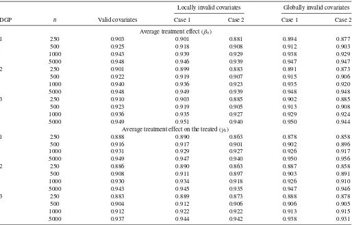
Table 4shows the empirical coverage of the 95% confidence intervals of the CSC average estimator based on the asymptotic distribution in Section3. When the sample sizenis small, we often have slight undercoverage. However, as the sample sizen increases, the empirical coverage becomes close to the nominal 95%.

6.2 Locally Invalid Covariates

We consider the case where some sets of covariates are locally invalid. Again, we consider five sets of covariates. The first setX1=(X∗, X1, X2, X3, X4) is the benchmark set of valid

(13)

Table 3-2. Relative efficiency: globally invalid covariates—Case 2

CSC Smoothed CSC

1 250 1.000 1.317 4.314 1.329 4.302 1.026 1.079 1.086

500 1.000 2.138 8.368 2.176 8.320 1.124 1.186 1.191

1000 1.000 4.053 17.249 4.027 17.293 1.187 1.175 1.179

5000 1.000 17.712 84.595 17.626 84.588 1.023 1.000 1.000

2 250 1.000 1.030 2.915 1.029 2.910 0.997 1.114 1.055

500 1.000 1.583 5.543 1.619 5.507 1.085 1.382 1.149

1000 1.000 2.807 11.117 2.796 11.118 1.193 1.650 1.236

5000 1.000 11.806 54.915 11.737 54.975 1.041 1.374 1.000

3 250 1.000 0.837 1.776 0.851 1.779 0.899 0.958 0.959

500 1.000 1.103 2.913 1.087 2.875 0.974 1.033 1.033

1000 1.000 1.621 5.157 1.606 5.186 1.071 1.145 1.146

5000 1.000 5.095 22.316 5.068 22.249 1.109 1.065 1.065

1 250 1.000 0.895 2.968 0.903 2.931 0.938 1.022 1.029

500 1.000 1.598 6.294 1.625 6.254 1.080 1.178 1.188

1000 1.000 3.086 13.158 3.077 13.224 1.260 1.340 1.348

5000 1.000 13.448 64.211 13.388 64.228 1.087 1.014 1.015

2 250 1.000 0.737 2.384 0.735 2.352 0.901 0.880 0.992

500 1.000 1.248 4.908 1.281 4.877 1.037 1.172 1.143

1000 1.000 2.386 10.352 2.381 10.402 1.226 1.475 1.321

5000 1.000 10.714 53.147 10.652 53.234 1.139 1.491 1.036

3 250 1.000 0.607 0.852 0.615 0.853 0.795 0.875 0.875

500 1.000 0.760 1.267 0.753 1.241 0.852 0.935 0.936

1000 1.000 1.002 1.951 0.999 1.965 0.949 1.056 1.056

5000 1.000 2.454 6.914 2.443 6.897 1.213 1.343 1.344

covariates. For the remaining four sets of covariates, we consider two cases:

Case 1:X2=(X∗, X1),X3=(X∗, X2),X4=

X†, X3

and X5 =

X†_{, X}

4

,where X†₌X∗₊_√1

n

(1+D) (1+U)+ǫ†, (10)

andǫ†is a standard normal random variable. HereX1,X2,

andX3 are three sets of valid covariates.X4 andX5 are

locally invalid, as the presence of _√1

n[(1+D)(1+U)+ǫ †_]_in_X†

makes the unconfoundedness assumption invalid for any finiten.HoweverX†_approaches_X∗_when_n_{goes to infinity.}

Here,J0=3.For the implementation details of our average

estimator whenJ0>1,see Remark 8.

Case 2:X2=(X†, X1),X3=(X†, X2),X4=(X†, X3), and

X5 =(X†, X4),whereX† is as defined in Equation (10).

In this case, we only have one set of valid covariates:X1

and four sets of locally invalid covariates:X2,X3,X4, and

X5,that is,J0 =1.

Table 2-1 presents the relative efficiency of different esti-mators for Case 1. Compared with the estimator based on the benchmark covariate set 1, in general, the estimator based on covariate set 2 performs better, while those based on covari-ate sets 3 and 5 perform worse. The relative performance of the estimator based on covariate set 4 depends on the sam-ple size. It is interesting to note that sometimes the estimators

based on locally invalid covariates outperform those based on valid covariates. For most DGPs and sample sizes, the perfor-mance of our CSC average estimator is the best among all three data-driven methods. The MSE is reduced by about 5%–35% compared with that when the estimator based on the first set of covariates is used. Both the smoothed average estimator and the selected estimator perform better than the estimator based on the benchmark covariate set 1.

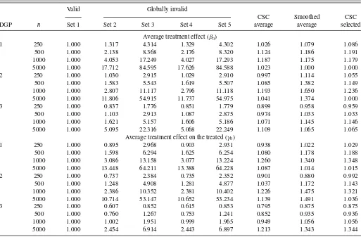
Table 2-2shows the relative performance of the estimators for Case 2. Compared with Case 1, covariate sets 2 and 3 also become locally invalid, thus the performances of the estimators based on them deteriorate. As a consequence, the performances of all three data-driven methods deteriorate. However, our CSC average estimator still outperforms the estimator based on the benchmark covariate set 1, and can reduce the MSEs by about 5%–15%.

Table 4reports the empirical coverage of the 95% confidence intervals of the CSC average estimator for both cases using the simple method (Equation (6)) withK₌1000. The actual coverage is close to the nominal coverage of 95% when the sample size is large.

6.3 Globally Invalid Covariates

Even though our theoretical results do not apply to globally invalid covariates, in practice, our CSC can still be used. We consider two cases involving globally invalid covariates:

(14)

Table 4. Empirical coverage of 95% confidence intervals for CSC average estimators

Locally invalid covariates Globally invalid covariates

DGP n Valid covariates Case 1 Case 2 Case 1 Case 2

1 250 0.903 0.901 0.881 0.894 0.877

500 0.925 0.918 0.908 0.912 0.903

1000 0.943 0.939 0.929 0.938 0.929

5000 0.948 0.946 0.939 0.947 0.947

2 250 0.901 0.899 0.883 0.891 0.873

500 0.922 0.919 0.907 0.915 0.906

1000 0.940 0.936 0.923 0.935 0.920

5000 0.948 0.949 0.939 0.948 0.948

3 250 0.910 0.903 0.885 0.902 0.885

500 0.923 0.919 0.905 0.913 0.908

1000 0.936 0.935 0.927 0.929 0.924

5000 0.949 0.951 0.940 0.950 0.944

1 250 0.888 0.890 0.863 0.878 0.858

500 0.916 0.917 0.901 0.902 0.896

1000 0.931 0.929 0.927 0.926 0.917

5000 0.949 0.947 0.940 0.950 0.956

2 250 0.886 0.890 0.863 0.887 0.858

500 0.908 0.911 0.897 0.903 0.891

1000 0.930 0.934 0.918 0.926 0.910

5000 0.943 0.945 0.935 0.947 0.946

3 250 0.883 0.889 0.873 0.888 0.878

500 0.904 0.912 0.906 0.906 0.905

1000 0.912 0.922 0.922 0.913 0.915

5000 0.937 0.944 0.942 0.938 0.931

Case 1: X2=(X∗, X1), X3=(X∗, X2), X4=(X3), and

X5=(X4).It is easy to see thatX1,X2andX3are valid,

whileX4andX5are globally invalid. Thus,J0=3.

Case 2:X2=(X1),X3=(X2),X4=(X3), andX5=(X4).

Here we only have one set of valid covariates:X1and four

sets of globally invalid covariates:X2, X3,X4, and X5.

Thus,J0=1.

Table 3-1presents the relative efficiency for Case 1. Appar-ently, when the sample size is relatively large, the estimators based on the globally invalid covariate sets 4 and 5 perform much worse than those based on the valid covariate sets 1, 2, and 3. For example, for DGP 1 (ATE) andn₌5000,the MSE

based on covariate set 5 is 84 times larger than that based on covariate set 1. However, when the sample size is small, some-times the estimators based on the globally invalid covariates outperform those based on the valid covariates. Our CSC aver-age estimator performs well, and beats the estimator based on the benchmark covariate set 1 for all DGPs and all sample sizes. Table 3-2reports the relative performance for Case 2. Com-pared with Case 1, covariate sets 2 and 3 also become globally invalid. Thus for large sample sizes, the estimators based on covariate sets 2–5 are all much worse than that based on the benchmark covariate set 1. Even in this case, our average CSC estimator still performs slightly better than or is comparable to the estimator based on the valid covariate set 1 when the sample

Table 5. Weights in CSC average estimators: globally invalid covariates—Case 2

DGP n Set 1 Set 2 Set 3 Set 4 Set 5

1 5000 0.975 0.013 0.000 0.013 0.000

2 5000 0.960 0.020 0.000 0.020 0.000

3 5000 0.871 0.068 0.000 0.061 0.000

1 5000 0.945 0.028 0.000 0.028 0.000

2 5000 0.924 0.038 0.000 0.038 0.000

3 5000 0.536 0.232 0.001 0.230 0.001

NOTE: The numbers in the main entries are the mean weights of the individual estimators in the CSC average estimators over 5000 replications.

(15)

Table 6-1. Outcome and treatment

Name Description

Y Difference in

OROA

the three year average of industry- and performance-adjusted OROA after CEO transitionsminusthe three-year

average before CEO transitions

D Family CEO ₌1 if the incoming CEO of the firm is

related by blood or marriage to the departing CEO, to the founder,

larger shareholder

=0 otherwise

size is small, and performs only slightly worse when the sam-ple size is large. Apparently, the performance of our average estimator deteriorates as we add more sets of globally invalid covariates, but is still within a reasonable range even when the majority sets of covariates are globally invalid.

In Remark 7, we argue that for large samples, our method should assign a weight close to zero to the estimators based on globally invalid covariates. We can confirm this through simulations.Table 5reports the mean weights of each individual estimator in our average estimators (over 5000 replications) for Case 2 withn₌5000. For most DGPs, our method assigns very small weights to the estimators based on the globally invalid covariates. For example, for ATE in DGP 1, the first estimator based on the benchmark valid covariates receives a weight of 97.5%, while the other four estimators based on the globally invalid covariates all receive a weight close to 0.

Table 4shows the empirical coverage of the 95% confidence intervals for both cases. Again, the actual coverage approaches the nominal coverage of 95% when the sample size increases.

The simulation results above suggest that our method can be applied to globally invalid covariates, even though our theory applies to locally invalid covariates only.

Remark 10. So far, we have only considered the case where the number of candidate sets of covariates (J) is fixed. As a referee suggests, it would be interesting to consider the case whereJincreases with the sample size (n).Therefore, we also letJ ₌Jn= ⌊n1/3⌋for all cases considered above, where⌊·⌋

denotes the integer part of·. Our average estimator performs sim-ilarly well in the increasingJcase. To save space, the detailed results are not reported here, but are available upon request. The asymptotic theory for the increasingJcase is, however, quite involved. For example, the variance–covariance matricesVβand

Vγ become high dimensional. To estimate them, some

regular-ization is often needed (see, e.g., Bickel and Levina2007). We leave the rigorous theoretical analysis for the increasingJcase for future research.

Remark 11. In an earlier version of this article, we also con-sidered a case where the benchmark set of covariates is small. However, as an associate editor and a referee kindly point out that in practice, researchers often use a large set of covariates. Therefore we consider the DGPs above. The results for the case where a small set of covariates is used as a benchmark are available upon request.

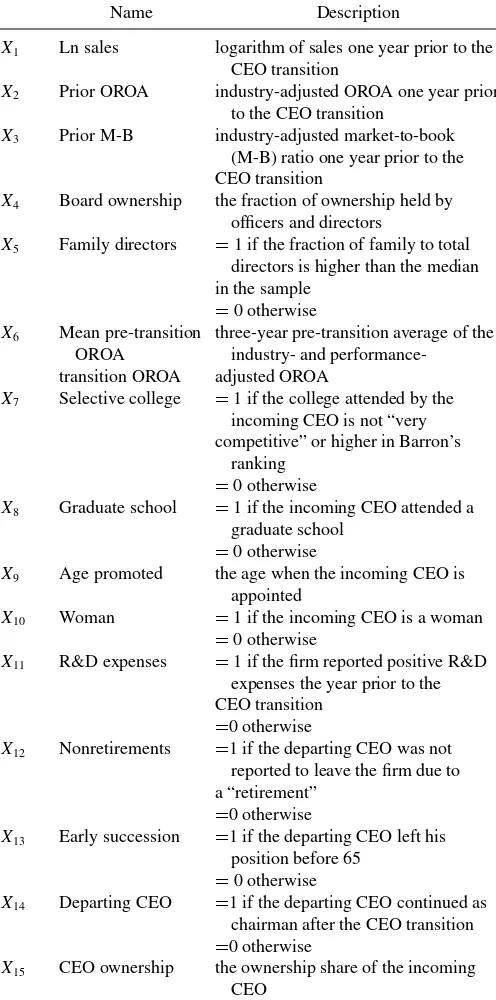
Table 6-2. Covariates (X)

Name Description

X1 Ln sales logarithm of sales one year prior to the

CEO transition

X2 Prior OROA industry-adjusted OROA one year prior

to the CEO transition

X3 Prior M-B industry-adjusted market-to-book

(M-B) ratio one year prior to the CEO transition

X4 Board ownership the fraction of ownership held by

officers and directors

X5 Family directors ₌1 if the fraction of family to total directors is higher than the median in the sample

=0 otherwise

X6 Mean pre-transition

OROA

three-year pre-transition average of the industry- and

performance-transition OROA adjusted OROA

X7 Selective college ₌1 if the college attended by the incoming CEO is not “very competitive” or higher in Barron’s

ranking

=0 otherwise

X8 Graduate school ₌1 if the incoming CEO attended a

graduate school

=0 otherwise

X9 Age promoted the age when the incoming CEO is

appointed

X10 Woman ₌1 if the incoming CEO is a woman

=0 otherwise

X11 R&D expenses ₌1 if the firm reported positive R&D expenses the year prior to the CEO transition

=0 otherwise

X12 Nonretirements ₌1 if the departing CEO was not

reported to leave the firm due to a “retirement”

=0 otherwise

X13 Early succession ₌1 if the departing CEO left his position before 65

=0 otherwise

X14 Departing CEO ₌1 if the departing CEO continued as

chairman after the CEO transition

=0 otherwise

X15 CEO ownership the ownership share of the incoming

CEO

7. EMPIRICAL APPLICATIONS

We apply our method to study the effects of inherited family control on firm performance as in Pérez-González (2006) and Lu and White (2014). Specifically, we are interested in whether firms with familiarly related incoming chief executive officers (CEOs) underperform relative to firms with unrelated incoming CEOs in terms of the firms’ operating return on assets (OROA). We use the data on 335 management transitions of publicly traded U.S. corporations as in Pérez-González (2006). Both Pérez-González (2006) and Lu and White (2014) used linear regressions. Here, we consider the semiparametric estimation

(16)

Table 7. Sets of covariates

Set Covariates

Set 1 (X1) {X2, X4, X5}

Set 2 (X2) {X1, X2, X3, X4, X5, X6}

Set 3 (X3) (X2, X4, X5, X7,X8, X9, X10)

Set 4 (X4) {X2, X4, X5, X11}

Set 5 (X5) {X2, X4, X5, X12, X13, X14, X15}

of ATE and ATT.Tables 6-1and6-2are the same as those in Lu and White (2014) and describe the outcomes (Y), treatment (D) and 15 covariates (X).

We consider the five candidate sets of covariates listed in Table 7, which are exactly the same as those in Lu and White (2014). We first assume that all five sets of covariates are valid. Then we assume some covariates are locally invalid. Lu and White (2014) called the first set of covariates (X1) core

covari-ates, thus we treat it as the only valid set of covariates and treat all other sets of covariates as locally invalid. (We also try treat-ing other sets of covariates as valid covariates and find similar results.) Lu and White (2014) provided a detailed discussion on how these five sets of covariates are chosen. For brevity, we omit the details here.

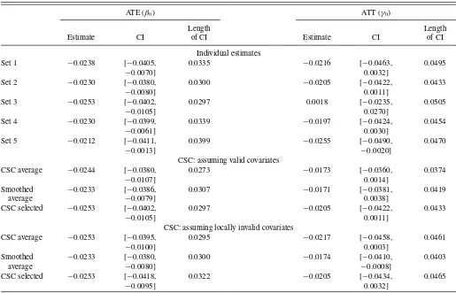
The estimation of ATE and ATT is implemented in the same way as in the simulation. In this application, we have many binary covariates. Given the relatively small sample size, these binary variables enter the sieve terms linearly (i.e., without in-teracting with those continuous covariates).Table 8reports the estimation results. For ATE, all individual estimates are negative and significant at the 5% significance level. Our CSC average estimate assuming all sets of covariates are valid is −0.0244 with the 95% confidence interval of [−0.0380,−0.0107]. The CSC average estimate assuming that covariate sets 2–5 are lo-cally invalid is₋0.0253 with the 95% confidence interval of [−0.0395,−0.0100].

For ATT, all the individual estimates are negative except that based on covariate set 3. However, they are not significant at the 5% level except that based on covariate set 5. If we as-sume that all covariates are valid, then our CSC average esti-mate is−0.0173 with the 95% confidence interval of [−0.0360, 0.0014]. If we assume that covariate sets 2–5 are locally invalid, our CSC average estimate is−0.0217 with the 95% confidence interval of [−0.0458, 0.0003]. This suggests that ATT is not significant at the 5% level.

Note that in general, our CSC average estimator has nar-rower confidence intervals than the individual estimators. This suggests the efficiency gains of our new estimator. We also implement the Hausman-type test for Hypotheses 1 and 2

Table 8. Estimation of ATE and ATT

ATE (β0) ATT (γ0)

Length Length

Estimate CI of CI Estimate CI of CI

Individual estimates

Set 1 ₋0.0238 [₋0.0405,

−0.0070]

0.0335 ₋0.0216 [₋0.0463,

0.0032]

0.0495

Set 2 ₋0.0230 [₋0.0380,

−0.0080]

0.0300 ₋0.0205 [₋0.0422,

0.0011]

0.0433

Set 3 ₋0.0253 [₋0.0402,

−0.0105]

0.0297 0.0018 [₋0.0235,

0.0270]

0.0505

Set 4 ₋0.0230 [₋0.0399,

−0.0061]

0.0339 ₋0.0197 [₋0.0424,

0.0030]

0.0454

Set 5 ₋0.0212 [₋0.0411,

−0.0013]

0.0399 ₋0.0255 [₋0.0490,

−0.0020]

0.0470

CSC: assuming valid covariates

CSC average ₋0.0244 [₋0.0380,

−0.0107]

0.0273 ₋0.0173 [₋0.0360,

0.0014]

0.0374

Smoothed average

−0.0233 [₋0.0386,

−0.0079]

0.0307 ₋0.0171 [₋0.0381,

0.0038]

0.0419

CSC selected ₋0.0253 [₋0.0402,

−0.0105]

0.0297 ₋0.0205 [₋0.0422,

0.0011]

0.0433

CSC: assuming locally invalid covariates

CSC average ₋0.0253 [₋0.0395,

−0.0100]

0.0295 ₋0.0217 [₋0.0458,

0.0003]

0.0461

Smoothed average

−0.0233 [₋0.0380,

−0.0080]

0.0300 ₋0.0174 [₋0.0410,

−0.0008]

0.0403

CSC selected ₋0.0253 [₋0.0418,

−0.0095]

0.0322 ₋0.0205 [₋0.0434,

0.0032]

0.0465

NOTE: CI stands for 95% confidence interval.