Full Terms & Conditions of access and use can be found at
http://www.tandfonline.com/action/journalInformation?journalCode=ubes20
Download by: [Universitas Maritim Raja Ali Haji] Date: 11 January 2016, At: 19:36
Journal of Business & Economic Statistics
ISSN: 0735-0015 (Print) 1537-2707 (Online) Journal homepage: http://www.tandfonline.com/loi/ubes20
Decomposing the Composition Effect: The Role
of Covariates in Determining Between-Group
Differences in Economic Outcomes
Christoph Rothe
To cite this article: Christoph Rothe (2015) Decomposing the Composition Effect: The Role of Covariates in Determining Between-Group Differences in Economic Outcomes, Journal of Business & Economic Statistics, 33:3, 323-337, DOI: 10.1080/07350015.2014.948959
To link to this article: http://dx.doi.org/10.1080/07350015.2014.948959
Published online: 17 Jul 2015.
Submit your article to this journal
Article views: 158
View related articles
Decomposing the Composition Effect: The Role
of Covariates in Determining Between-Group
Differences in Economic Outcomes
Christoph R
OTHEDepartment of Economics, Columbia University, New York, NY 10027([email protected])
In this article, we study the structure of the composition effect, which is the part of the observed between-group difference in the distribution of some economic outcome that can be explained by differences in the distribution of covariates. Using results from copula theory, we derive a new representation that contains three types of components: (i) the “direct contribution” of each covariate due to between-group differences in the respective marginal distributions, (ii) several “two-way” and “higher-order interaction effects” due to the interplay between two or more marginal distributions, and (iii) a “dependence effect” accounting for between-group differences in dependence patterns among the covariates. We show how these components can be estimated in practice, and use our method to study the evolution of the wage distribution in the United States between 1985 and 2005. We obtain some new and interesting empirical findings. For example, our estimates suggest that the dependence effect alone can explain about one-fifth of the increase in wage inequality over that period (as measured by the difference between the 90% and the 10% quantile).
KEY WORDS: Detailed decomposition; Counterfactual distribution; Copula; Wage inequality; Labor market polarization.
1. INTRODUCTION
Understanding the factors accounting for the differences in the distributions of individuals’ economic outcomes across two countries, time periods, or subgroups of the population is central in several fields of economic research, particularly in labor and development economics. For instance, the question of why wage inequality has increased substantially in the United States and other industrialized countries over the past decades has received enormous attention in the recent literature. Other examples in-clude the study of the gender wage gap, wage differentials be-tween natives and immigrants, and variations in health outcomes across several developing regions. The distributional aspect is often critical in these applications. Comparing real hourly wages among male U.S. workers in 1985 and 2005, for example, one can observe that the median wage has remained approximately constant, but that the 90% and 10% quantile have increased by about 20% and 5%, respectively. There has thus been a substan-tial change in the overall shape of the wage distribution, which would not be revealed by a simple comparison of means.
With such applications in mind, a number of articles have proposed procedures to decompose between-group differences in economic outcomes into two components: a composition ef-fect due to differences in observable covariates across groups, and a structure effect due to differences in the relationship that links the covariates to the outcome. The most popular example is certainly the Oaxaca–Blinder procedure (Blinder1973; Oax-aca1973) for decomposing differences in mean outcomes when the data are generated by a simple linear model. More flexible methods that can be used to decompose general distributional features like quantiles or inequality measures, and allow for complex nonlinear relationships between the covariates and the outcome variable are proposed and studied by DiNardo, Fortin, and Lemieux (1996), Gosling, Machin, and Meghir (2000),
Donald, Green, and Paarsch (2000), Barsky et al. (2002), Machado and Mata (2005), Rothe (2010), and Chernozhukov, Fernandez-Val, and Melly (2013), among others. See Fortin, Lemieux, and Firpo (2011) for a literature review.
A natural question in empirical applications is whether the composition effect can be further decomposed into contribu-tions attributable to specific covariates. For example, it could be interesting to know what portion of the composition part of the wage gap between natives and immigrants can be attributed to between-group differences in education. Further decompo-sitions of between-group differences in mean outcomes can be obtained via the Oaxaca–Blinder procedure when the data are generated by a linear model. For more general settings, alter-native further decompositions have been proposed and studied by, for example, DiNardo, Fortin, and Lemieux (1996), Altonji, Bharadwaj, and Lange (2012), or Chernozhukov, Fernandez-Val, and Melly (2013), among many others. These methods are generallypath dependent, in the sense that their results depend on the order of the covariates in the dataset, which can be un-desirable in many applications where there is no natural order among the covariates. More importantly, the elements of these further decompositions typically measure the contribution of between-group differences in theconditionaldistribution of a covariate given the remaining ones, and can thus not be in-terpreted as reflecting between-group differences in a single, specific covariate.
It turns out that it is not possible to develop a general method that apportions the composition effect into components that are only attributable to between-group differences in the marginal
© 2015American Statistical Association Journal of Business & Economic Statistics
July 2015, Vol. 33, No. 3 DOI:10.1080/07350015.2014.948959
323
distribution of specific covariates in such a way that these components add up to the full composition effect. This is be-cause most commonly used distributional features other than the mean, such as the variance, quantiles, or inequality measures, are nonlinear transformations of the distribution of the outcome variable, and are thus not additively separable in the marginal distributions of the covariates. Instead, they typically contain “interaction terms” that stem from the interplay of two or more covariates’ marginal distributions, and are also influenced by between-group differences in the dependence patterns among the covariates. This is generally true even if the underlying data-generating process (DGP) does not contain any interac-tion terms itself. For example, when the data are generated by a simple linear model, between-group differentials in the out-comes’ variances can be due to between-group differences in covariances among the explanatory variables. Since the covari-ance of two random variables is the product of their respective standard deviations and the correlation coefficient, it depends on features of both covariates’ marginal distributions, and on the dependence structure between them. Such terms cannot be apportioned unambiguously to specific covariates.
The main contribution of this article is to derive a new de-composition of the de-composition effect that explicitly takes these issues into account. In particular, the decomposition contains three types of components: (i) the “direct contribution” of each covariate due to between-group differences in the respective marginal distributions, (ii) several “two-way” and “higher-order interaction effects” due to the interplay between two or more marginal distributions, and (iii) a “dependence effect” account-ing for different dependence patterns among the covariates. We show that such a decomposition is well defined in a general set-ting by using results from copula theory (e.g., Nelsen2006) and arguments related to those in Rothe (2012). Under suitable ex-ogeneity conditions, these components can all be interpreted in terms of economically meaningful counterfactual experiments that change the joint distribution of the covariates to a hypothet-ical one that shares properties of both groups (Rothe2012).
To gain a better understanding of the empirical content of our decomposition, it is useful to consider a simple example. Suppose that we study the populations of workers in countries A and B, that our outcome variable is the hourly wage, and that there are two covariates: the worker’s age and an indicator for union coverage. To be concrete, also suppose that population A tends to be older and more unionized, and that union coverage is more attractive for relatively old workers in population A than it is in population B. Then the composition effect is the part of the wage gap between the two populations that can be explained by these differences in observable characteristics. The first “direct contribution” is then the part of the composition effect that can be attributed to the fact that population A tends to be older. The second “direct contribution” accounts for population A having higher unionization rates. The (only) “interaction effect” mea-sures theadditionalcontribution of the fact that the population A isbothmore unionized and older. Finally, the “dependence effect” captures the fact that the relative age composition of union-covered and nonunion-covered workers differs in the two populations.
An attractive feature of our decomposition is that it reduces to the Oaxaca–Blinder procedure for the special case of the mean
of the outcome in a linear regression model. It can thus be under-stood as a natural extension of this method to nonlinear models and general distributional features. We also show in this article that the elements of our decomposition are conceptually easy to estimate in a flexible parametric framework, requiring only standard statistical methods to estimate copula functions and conditional CDFs. The asymptotic variance of these estimates generally has a complicated form, but valid standard errors can be computed via a classical bootstrap approach.
As an additional contribution, we also apply our new method-ology to study the evolution of the wage distribution among male workers in the United Stated between 1985 and 2005. There is now extensive evidence that during this period wage inequal-ity in the United States has been rising substantially in the top end of the wage distribution, but has slightly decreased in the bottom end, leading to what is often called a polarization of the U.S. labor market (Autor, Katz, and Kearney 2006; Lemieux 2008). Our methodology delivers some new and interesting in-sights into this issue. For example, our estimates suggest that our dependence effect, which has no analog in other methods, accounts for about one-fifth of the increase in wage inequal-ity (as measured by the difference between the 90% and the 10% quantile) that occurred over the two decades, and about one-fourth of the composition effect. This dependence effect captures, for example, changes in the positions of unionized and nonunionized workers in the age distribution.
It should be stressed that our focus in this article is exclusively on a decomposition of the composition effect. We do not address the related issue of deriving a decomposition of the structure effect, that is, dividing between-group differences in the struc-tural functions that link the covariates and the outcome variable into components that can be attributed to individual covariates. Such a task already faces conceptual difficulties in simple linear models with discrete covariates, and does not seem possible for general nonlinear structural functions with interactions between the covariates.
The remainder of the article is structured as follows. In the next section, we introduce a general setting for studying struc-ture and composition effects, and illustrate the conceptual diffi-culties for decomposing the composition effect through a sim-ple examsim-ple. In Section3, we describe our new decomposition based on copulas. Section 4 compares our approach to other approaches that have been proposed in the literature. Section 5 shows how to estimate the elements of our decomposition in practice, and Section6derives the asymptotic properties of these estimators. Section7contains an empirical application to wage data from the United States. Finally, Section8concludes. Some proofs and more extensive calculations are given in the Appendices.
2. STRUCTURE AND COMPOSITION EFFECTS
2.1 General Setup
We consider a population with two nonoverlapping subgroups indexed byg∈ {0,1}. For any individual in groupg, we observe an outcome variableYg and ad-dimensional vector of
observ-able characteristicsXg, with corresponding distribution
func-tionsFYgandFXg, supportYgandXg, and conditional CDFFg Y|X,
respectively. Furthermore, for any CDFF, we refer to objects of the formν(F) as a distributional feature, whereν:F→Ris a functional from the space of all one-dimensional distribution functions to the real line. Examples of distributional features include the mean, withν:F →ydF(y), and theτ-quantile, with ν:F →F−1(τ), but also higher-order centered or un-centered moments, quantile-related statistics like interquantile ranges or quantile ratios, and inequality measures such as the Gini coefficient. Our aim is to understand how the observed difference
νO=νFY1−νFY0
between the distributional featuresν(F1
Y) and ν(F
0
Y) is related
to differences between the distributionsF1
XandF
0
X. To this end,
we define a counterfactual outcome distributionFYg|j that com-bines the conditional distribution in groupgwith the covariate distribution in groupj =g:
FYg|j(y)=FYg|X(y, x)dFXj(x). (2.1) This integral is well defined as long asXj ⊂Xg. We interpret
FYg|j as the distribution of outcomes after a counterfactual ex-periment in which the distribution of observable characteristics in groupgis changed fromFXgtoFXj, but the conditional distri-bution of the outcome given these characteristics remains con-stant. With the notation (2.1), one can decompose the observed between-group differentialνOas
νO =ν S+
ν
X, (2.2)
where
νS=ν(FY1)−ν(FY0|1) andνX=ν(FY0|1)−ν(FY0).
Hereν
X is a composition effect, solely due to differences in
the distribution of the covariates between the two groups, and
ν
S is a structure effect, solely due to differences in the
con-ditional CDFsF1
Y|XandF
0
Y|X. This definition of structure and
composition effects has been widely used in the literature (e.g., DiNardo, Fortin, and Lemieux1996; Machado and Mata2005; Rothe2010; Chernozhukov, Fernandez-Val, and Melly 2013, among many others). We note that the order in which differ-ences in conditional CDFs and the covariate distributions are considered when definingνX andνShas to be taken into ac-count when interpreting the parameters in practice.
To give a concrete example that fits our setting, suppose that group 0 and 1 are the population of male workers in 1985 and 2005, respectively,Ygis an individual’s wage in constant 1985
dollars, Xg are observable characteristics that are relevant on
the job market, andν is some measure of inequality. In this case, the conditional CDFFYg|Xsummarizes the wage schedule given the worker’s observable characteristics in periodg, and
FYg|j is the counterfactual distribution of wages that would have prevailed if the distribution of workers’ characteristics in period
gwould have been the same as in periodj. Moreover,νXandνS
quantify to what extent changes in wage inequality over time, as measured byνO, can be attributed to the evolution of workers’ characteristics and changes in the wage schedule, respectively.
Note that the structure and composition effects can be given a causal interpretation under (arguably strong) exogeneity con-ditions on the covariates. Specifically, suppose that the out-come variable is generated through the nonseparable model
Yg=mg(Xg, ηg) for g∈ {0,1}, where ηg∈Rdη is an
unob-served error term andmgis the structural function. Now ifηgis independent ofXg, then for anyd-dimensional CDFGwe can interpret the functionHG(y)=
FYg|X(y, x)dG(x) as the CDF of the counterfactual random variablemg(Z, ηg), whereZ∼G
is ad-dimensional random vector that is independent ofηg.
2.2 Problems for Decomposing the Composition Effect
When the data contain information about several individual characteristics, it is natural to ask which role between-group differences in each one of them play in determining the compo-sition effect. For example, one could be interested to which ex-tent the composition part of the change in wage inequality from 1985 to 2005 can be attributed to the decline in unionization, the change in the distribution of workers’ age, etc. Such ques-tions can easily be addressed for the mean of the outcome vari-able in a simple linear model by the Oaxaca–Blinder procedure, which certainly contributes to the popularity of the method. This method does not apply, however, to other distributional features such as quantiles or variances, or more complex relationships between the outcome and the covariates.
It would thus be desirable to have a methodology that is able to apportion the composition effect into components attributable to between-group differences in the marginal distribution of each covariate in the general setting described above. However, it is clear that such a decomposition does generally not exist when the distributional feature of interest is a nonlinear trans-formation of the CDF of the outcome variable. This is the case for essentially all features commonly used in empirical appli-cations, with the exception of the mean. These nonlinearities create issues even for simple DGPs like linear models. To see this, consider the following simple example. Suppose that in both groups, that is, for anyg∈ {0,1}, the data are generated as
Yg
=Xg1+X2g+ηg, whereXg
∼N(µg, g) is bivariate
nor-mal with
µg =
µg1
µg2
andg =
σg21 ρgσg1σg2
ρgσg1σg2 σg22
,
and ηg∼N(0,1) is independent of Xg. Since the
struc-tural function is the same in both groups, we clearly have that ν
S=0 for any functional ν, and thus any difference
in the distribution of Y1 and Y0 reflects a composition
ef-fect. For instance, if ν(FYg)=var(Yg), we have that ν X=
var(Y1)−var(Y0) with var(Yg)=1+σg21+σg22+2ρgσg1σg2.
When ν(FYg)=QgY(τ) is theτ-quantile of the distribution of
Yg, we find that ν X=Q
1
Y(τ)−Q
0
Y(τ) with Q g
Y(τ)=µg1+
µg2+ −1(τ)
1+σg21+σg22+2ρgσg1σg2 and the CDF of
the standard normal distribution. In both cases, the object of interest is not additively separable in the parameters (µg1, σg21)
and (µg2, σg22), which characterize the covariates’ marginal
dis-tributions in this example. Moreover, in both cases the object of interest depends on the value of the correlation coefficientρg,
which determines the dependence structure among the covari-ates here.
3. CHARACTERIZING THE COMPOSITION EFFECT USING COPULAS
3.1 Preliminaries
It turns out that the simple example in Section2.2illustrates a general property of the composition effect: it is usually not possible to express the composition effect as a sum of terms that each depend on the marginal distributions of a single covariate only. Instead, an explicit expression of the composition effect in terms of the respective marginal covariate distributions typically contains “interaction terms” resulting from the interplay of two or more marginal distributions, and also “dependence terms” resulting from between-group difference in the dependence pat-tern among the covariates.
To formally show this point, we use results from copula the-ory that allow us to disentangle the covariates’ marginal distri-butions from the dependence structure among them. In particu-lar, it follows from Sklar’s Theorem (Sklar1959; Nelsen2006, Theorem 2.3.3) that the CDF ofXg can always be written as
FXg(x)=Cg(FXg
1(x1), . . . , F
g
Xd(xd)) forg∈ {0,1}, (3.1)
where Cg is a copula function, that is, a multivariate CDF
with standard uniformly distributed marginals, and FXg k is the
marginal distribution of thekth component ofXg. The copula
describes the joint distribution of individuals’ ranks in the vari-ous components ofXg, and can be interpreted as the object that
determines the dependence structure.
To ensure that the definition of Cg is unique on its entire
domain [0,1]d, we assume that the covariatesXg can be
rep-resented asXg =t( ˜Xg)=(t1( ˜X
g
1), . . . , td( ˜X g
d)) for some
con-tinuously distributed random vector ˜Xg and a function t(·) that is weakly increasing in each of its arguments. For ex-ample, if the lth component of Xg is binary, we could have
Xgl =I{X˜g
l > cl} =tl( ˜X g
l) for some constantcl. If thelth
com-ponent is continuously distributed, one can simply puttlas the
identity mapping. With such a structure, Cg can be uniquely
defined on [0,1]das the copula function of the joint CDF of the
latent variables ˜Xg. While this construction uniquely definesCg
on [0,1]d, it does of course not ensure thatCgis point identified
on [0,1]d from the distribution ofXg alone when some of the
covariates are discrete. We return to this issue in Section3.4. The representation (3.1) can be used to define counterfactual outcome distributions that combine the conditional distribution in group gwith hypothetical covariate distributions that share properties of both FX1 andFX0. Denoting any element of the
d-dimensional product set {0,1}d by a boldface letter, we define the distribution of the outcome in a counterfactual setting where the structure is as in groupg, the covariate distribution has the copula function of groupj, and the marginal distribution of thelth covariate is equal to that in groupklby
FYg|j,k(y)=FYg|X(y, x)dFXj,k(x) (3.2) with
FXj,k(x)=Cj(Fk1
X1(x1), . . . , F
kd
Xd(xd)).
Following the discussion at the end of Section 2.1, under suitable exogeneity conditions this distribution can be inter-preted as the one of the outcome variable in a counterfactual in which the distribution of the covariates is exogenously
shifted such that its new CDF is equal toFXj,k. We also write
1=(1,1, . . . ,1) and0=(0,0, . . . ,0), denote byelthelth unit
vector, that is, thed-dimensional vector whoselth component is equal to one and whose remaining components are equal to zero, and put|k| =d
l=1kl. Next, for any distributional feature
ν, we define the parameter
βν(k)=ν(F0|0,k
Y )−ν(F
0
Y),
which can be interpreted as the effect of a counterfactual experiment conducted in group 0 that changes the respective marginal distribution of those|k|covariates for whichkl=1
to their corresponding counterpart in group 1, while holding everything else (including the dependence structure among the covariates) constant. Note that the termβν(el) is an example of
a fixed partial distributional policy effects (FPPE) as introduced in Rothe (2012). Finally, we define
νM(k)=βν(k)+
1≤|m|≤|k|−1
(−1)|k|−|m|βν(m),
with the empty sum equal to zero, so that, for example,νM(el)
= βν(el). This notation will simplify the exposition below.
3.2 A Simple Example with Two Covariates
Before giving a general formula for our decomposition, it is instructive to first consider a simplified version where the vector of explanatory variablesXg has only two components, that is,
d=2. In this case, we can rewrite the composition effect as
νX =νM(e1)+ν
M(e
2
)+νM(1)+ν
D, (3.3)
where
νD =ν(FY0|1,1)−ν(FY0|0,1) and
νM(1)=βν(1)−βν(e1)−βν(e2).
The representation (3.3) conveys a number of insights into the structure of the composition effect. First, the termsνM(e1) and
νM(e2) can be interpreted as thedirectcontribution of
between-group differences in the marginal distribution of the first and second covariate to the composition effect, respectively. Sec-ond, the termν
M(1) can be interpreted as an interaction effect:
whileβν(1) measures thejoint contribution of between-group
differences in the marginal covariate distribution of between the two groups, subtractingβν(e1) andβν(e2) provides an
adjust-ment for thedirectcontribution of the first and second covariate, thus leading to the interpretation ofν
M(12) as a “pure”
inter-action effect. Third, the term ν
D is a dependence effect that
captures the contribution between-group differences in the co-variates’ copula functions. As a further illustration, in Appendix B we explicitly calculate the components of (3.3) for the simple setting described in Section2.2. An example how these terms can be interpreted in an empirical context was given in the in-troduction of this article.
3.3 A General Decomposition
We now describe a general decomposition of the compo-sition effect for high-dimensional settings, which is the main
contribution of this article. As a first step, the composition effect
ν
Xcan be decomposed into adependence effectνD resulting
from between-group differences in the copula functions, and a
total marginal distribution effectνM resulting from differences in the marginal covariate distributions across the two groups:
νX =νD+νM, (3.4) where
νD=ν(FY0|1,1)−ν(FY0|0,1) andνM =ν(FY0|0,1)−ν(FY0|0,0).
Note that the order in which differences in the copula and the marginal CDFs are considered when definingνD andνM has to be taken into account when interpreting the parameters in practice.
In a second step, we further decompose the total marginal distribution effectν
Minto severalpartial marginal distribution
effectsν
M(k), which account for between-group differences in
the marginal distributions of one or several covariates:
νM =
1≤|k|≤d
νM(k).
Note that the order of the covariates in the dataset has no impact on the numerical value of each of the ν
M(k), and that these
terms have been carefully defined in the previous section to avoid counting certain contributions more than once.
Taken together the various terms we just introduced, our full decomposition of the composition effect is given by
νX=
1≤|k|≤d
νM(k)+ν
D. (3.5)
In case|k| =1, that is, whenk=el is thelth unit vector, the
interpretation ofν M(e
l) is, as described above, that of a direct
contribution of between-group differences in the marginal dis-tribution of thelth covariate to the composition effect. For any vectork with|k|>1, the terms ν
M(k) capture the
contribu-tions to the composition effect of “|k|-way interaction effects”
between the marginal distributions for which respective compo-nent ofkis equal to one.
It should be stressed that the decomposition (3.5) is not merely a statistical identity. As discussed in Section2.1, under a suit-able exogeneity condition on the covariates, the termsνD and
νM(el) forl∈ {1, . . . , d}are all direct summary measures of the
outcome of well-defined counterfactual experiments, namely, that of aceteris paribus change in the copula function or the
lth marginal distribution, respectively. The terms of the form
ν
M(k) with|k|>1 arise from a comparison of the outcomes
of several counterfactual experiments that all involve ceteris paribus changes of two or more covariates’ marginal distri-butions. Thus, all elements of the decomposition (3.5) can be interpreted in terms of empirically meaningful counterfactual experiments.
3.4 Identification
It is easy to see that the elements of the decomposition (3.5) are well-defined as long as the support ofX1is contained in the
support ofX0, that is,X1⊂X0. When some of the covariates
are discrete, however, one generally requires further conditions
on the DGP to point-identify these quantities from the distri-bution of the observables. This is because the data identify the copula functionC0on the range of the respective marginal
dis-tribution functions of the components ofX0 only. There could
thus be several copula functions ˜C that satisfy the relationship
FX0(x)=C˜(FX0
1(x1), . . . , F
0
Xd(xd)) for allx∈ Rd
if some of the components ofX0are discrete (Nelsen2006). As a consequence,
there might be no one-to-one mapping between the distribution of observables and the counterfactual distributional features of the formν(FY0|0,s) withs∈ {0,1}d, which are required for
com-puting our decomposition. Note that this is not an issue if all covariates are continuously distributed.
In the presence of discrete covariates, one way to achieve point identification of the elements of the decomposition is by imposing certain parametric restrictions on the functional form of the copula. These restrictions can be very mild though, and still allow for a wide range of practically relevant dependence patterns. One might be willing to assume, for example, that
C0 belongs to the family of Gaussian copulas, or some other
family that satisfies a weak regularity condition that we state below. By making such an assumption, one reduces the class of values that C0 could potentially take such that it can be uniquely determined from the distribution of observables among the remaining candidates. The following proposition formalizes this argument.
Proposition 1. Suppose thatX1 ⊂X0, and that either of the following conditions hold:
1. The distribution functionF0
Xis continuous.
2. The copula functionC0
=Cθ0 is contained in the paramet-ric class {Cθ, θ ∈⊂Rk}, and it holds thatP(Cθ(U0)=
Cθ0(U0))>0 for U0=(FX01(X1,0), . . . , F
0
Xd(Xd,0)) and all θ∈\ {θ0}.
Then all terms in (3.5) are point-identified.
The statement of the proposition follows from elementary properties of copula functions (e.g., Nelsen2006) under con-dition (i), and from standard arguments for identification of parametric models (e.g., Newey and McFadden 1994) under condition (ii). The former condition is obviously straightfor-ward to verify, and the latter condition has testable implica-tions. If the parametric family of copula functions is such that
Cθ(u)=Cθ′(u) for allu∈(0,1)dand allθ=θ′, then condition
(ii) necessarily holds. This stronger sufficient condition can be shown to be fulfilled by most common parametric families of copula functions, such as, for example, the Gaussian, Clayton, or Frank family. In the absence of parametric restrictions, one could conduct a partial identification analysis similar to the one in Rothe (2012), and derive upper and lower bounds on the ele-ments of the decomposition (3.5). Whether or not these bounds would be sufficiently narrow to be informative in an empirical setting depends on the details of the respective application.
4. RELATIONSHIP TO OTHER APPROACHES
In this section, we compare our copula decomposition to sev-eral related approaches that have been proposed in the literature. We consider the classical Oaxaca–Blinder procedure, methods based on so-called sequential conditioning arguments, and a
method based on recentered influence function (RIF) regression that was recently proposed by Firpo, Fortin, and Lemieux (2007, 2013).
4.1 Decompositions Based on Linear Models
One important property of the decomposition (3.5) is that it encompasses the popular Oaxaca–Blinder procedure (Blinder 1973; Oaxaca1973) as a special case. Suppose that the data are generated as
Yg =β0g+
d
l=1
Xglβlg+ηg withE(ηg|Xg)=0,
and the expectation is the distributional feature of interest, that is,ν(FYg)=E(Yg
). Then it is straightforward to verify that the elements of our decomposition take the form
EM(el)=(E(X1l)−E(X0l))βl0, EM(k)=0 fork=eland
ED =0.
Our decomposition can thus be understood as a natural gener-alization of the Oaxaca–Blinder procedure to nonlinear DGPs and general features of the outcome distribution. Note that in this particular case the composition effect can be apportioned unambiguously into contributions attributable to each covariate as the additive separability of covariates in the DGP is preserved by the linearity of the functionalF →ydF(y) that maps a CDF into the corresponding expectation.
4.2 Decompositions Based on Sequential Conditioning Arguments
Our decomposition does generally not encompass meth-ods that are based on sequential conditioning arguments, such as those proposed by DiNardo, Fortin, and Lemieux (1996), Machado and Mata (2005), Altonji, Bharadwaj, and Lange (2012), or Chernozhukov, Fernandez-Val, and Melly (2013), for example. These approaches write the composition effect as a sum of terms that reflect changes in theconditional distribu-tion of one covariate given the remaining ones. That is, they start with the representation
FYg(y)=
FYg|X(y|x)dFXg1|X
−1(x1|x−1)
×dFXg
2|X−2(x2|x−2). . . dF
g Xd(xd),
wherea−kdenotes the subvector ofathat excludes its firstk
com-ponents, and consider counterfactual distributions obtained by exchanging the various conditional covariate distributions with their counterparts in the other group. As argued by Rothe (2012), such terms cannot be interpreted as the impact of between-group differences in the marginal distribution of particular covariates. In contrast to our method, these decompositions are alsopath dependent, in the sense that they depend on the order of the com-ponents ofXg. This property can be undesirable in applications
where there is no natural sequential order for the covariates.
4.3 Decompositions Based on RIF Regressions
Our approach is related to the RIF decomposition that was re-cently proposed by Firpo, Fortin, and Lemieux (2007,2013). To explain the connection, assume for a moment that all covariates are continuously distributed. Let RIF(Yg, ν) be the recentered influence function (Van der Vaart2000) ofν(FYg), and let
hg,ν(x)≡E(RIF(Yg, ν)|Xg =x)
be its conditional expectation function givenXg. Now define
γg,ν =E(∂xhg,ν
(Xg)) and ¯γg,ν =E(XgXg′)−1E(XgRIF(Yg, ν)),
which are the corresponding average derivative and the coeffi-cients of a linear projection of RIF(Yg, ν) ontoXg, respectively.
The latter can be understood as an approximation toγg,ν that
is easier to estimate in practice. The RIF decomposition of the composition effect is then given by
νX=
d
l=1
νM,RIF(l)+νE,RIF,
where
νM,RIF(l)≡γ¯l0,ν(E(X1
l)−E(X
0
l))
is interpreted as the contribution of thelth covariate andν E,RIF
is a residual term that is supposed to catch various types of misspecification.
Firpo, Fortin, and Lemieux (2009) showed that the compo-nents ofγg,ν measure the effect of infinitesimal location shifts
in the marginal distribution of the corresponding component of
Xg on ν(FYg), holding everything else (including the copula) constant. The termsνM,RIF(l) can thus be seen as “first-order” approximations to our ν
M(e
l) along a particular path in the
space of potential covariate distributions, namely, the one de-scribed by a location shift in thelth margin. This approximation should be adequate if (i) the distribution ofX1
l is close to a
location-shifted version of the distribution ofX0l, (ii) the loca-tion differenceE(X1
l)−E(X
0
l) is small, and (iii) ¯γ
0,ν
l is close to
γl0,ν. If one of these three conditions is violated thenνM,RIF(l) can differ fromνM(el) by a potentially large amount.
In cases where the approximation is inaccurate, the elements of the RIF decomposition do generally not correspond to mean-ingful population quantities. For example, suppose that the dis-tribution ofX1
l andX
0
l have the same mean but different
vari-ances, and are thus not location-shifted versions of each other. Thenν
M,RIF(l) is clearly equal to zero by construction even
though thelth covariate should in general contribute to the com-position effect for any distributional featureν that is affected by the spread of the covariate distribution. Note that checking whether the residual νE,RIF is small does not ensure the ac-curacy of the RIF approximation since it is easy to construct examples whereνE,RIF=0 butνM,RIF(l) differs fromνM(el)
for alllby an arbitrarily large amount.
5. MODEL SPECIFICATION AND ESTIMATION
In this section, we explain how our detailed decomposi-tion (3.4) and (3.5) can be estimated in practice. We focus on
flexible parametric specifications, which can be estimated using standard statistical techniques. Recall that for any distributional featureν the observed differenceνO, the structure effectνS, the dependence effectνD, and the various partial marginal dis-tribution effectsνM(k) can all be expressed in terms of objects
of the formν(FYg|j,k), where
FYg|j,k(y)=FYg|X(y, x)dCj(Fk1
X1(x1), . . . , F
kd
Xd(xd))
as defined in Equation (3.2). To obtain estimates of the elements of our decomposition, we can therefore use a plug-in approach and replace the termsν(FYg|j,k) at every occurrence with their
Xlbeing suitable estimates of the conditional
CDFFYg|X, the copula functionCg, and the marginal CDFsFg Xl
of thelth component ofXg, forg
∈ {0,1}andm∈ {1, . . . , d}, respectively. That is, our estimates are given by
for any distributional featureν. The integral on the right-hand side of Equation (5.1) can be approximated numerically through any of the many standard methods available in commonly used software packages.
We assume that the data available to the econometrician con-sist of two iid samples{(Yig, Xig)}ng
i=1of sizengfrom the
distribu-tion of (Yg, Xg) forg∈ {0,1}. In such a classical cross-sectional setting, estimates of the just-mentioned unknown functions can in principle be obtained by a variety of different methods. For the univariate distribution functionsFXg
l, the most straightforward
estimator is arguably the usual empirical CDF, which is given by
For the higher-dimensional objects, that is, the conditional CDFs and the copula functions, several nonparametric, semiparametric, and fully parametric procedures have been proposed in the literature. Since most studies that make use of decomposition methods use datasets containing a large number of individual sociodemographic characteristics, the substantial sample size requirements of nonparametric methods in such high-dimensional settings limit their attractiveness. We there-fore focus on flexible parametric specifications in this article, which have been applied successfully in the empirical literature. Our preferred method to estimate the conditional CDFsFYg|X, which is also used in our empirical application below, is the dis-tributional regression approach of Foresi and Peracchi (1995). The distributional regression model assumes that
FYg|X(y, x)≡ (x′δog(y)),
where (·) is the standard normal CDF (or some other strictly in-creasing link function). The finite-dimensional parameterδog(y)
can then be estimated by the maximum likelihood estimateδg(y)
in a Probit model that relates the indicator variableI{Yg
≤y}
The resulting estimate of the conditional CDF is then given by
FYg|X(y, x)= (x′δg(y)).
An alternative approach that is commonly found in the literature (e.g., Machado and Mata2005) would be to model the condi-tional quantile function by a linear quantile regression model (Koenker and Bassett 1978; Koenker 2005), and then invert the corresponding estimated quantile function. Chernozhukov, Fernandez-Val, and Melly (2013) derived asymptotic properties of conditional CDF estimators based on distributional and quan-tile regression (and several other parametric specifications), es-tablishing classical properties like√ng-consistency and
asymp-totic normality under standard regularity conditions. Rothe and Wied (2013) considered specification testing in these types of models.
The copula functionsCg can also be modeled a variety of
ways. Following the arguments preceding Proposition 1, we consider the case that Cg is contained in sufficiently flexible
parametric class indexed by ak-dimensional parameter, that is,
Cg ≡Cθog ∈ {Cθ, θ ∈⊂R
k
}.
Different parametric copula models are able to generate differ-ent types of dependence patters, and thus the analyst should chose a specification that is considered flexible enough to en-compass the relationship between the covariates in the respective group. The extensive reviews of the properties of various copula models in, for example, Nelsen (2006) or Trivedi and Zimmer (2007) are a useful guidance for this choice. When all covariates are continuously distributed, the dependence parameters of any common copula model can be estimated by maximum likelihood methods implemented in most common software packages, and estimates can be shown to be √ng-consistent and
asymptoti-cally normal under standard regularity conditions (e.g., Genest, Ghoudi, and Rivest1995). When some of the covariates follow a discrete marginal distribution, maximum likelihood estima-tion is still conceptually possible, but might not be feasible as the computational burden of evaluating the likelihood function grows exponentially in the number of discrete covariates and their support points (Joe1997). In empirical settings with large samples and many discrete covariates, it is therefore more prac-tical to use estimators for the copula parameters that are faster to compute, even though they might not be fully efficient. An ex-ample of an estimator that satisfies this criterion is the minimum distance estimator
where FXg denotes the joint empirical CDF of the covariate data from groupg. Other estimators for copula functions with discrete margins have recently been proposed, for example, by Nikoloulopoulos and Karlis (2009), Smith and Khaled (2012), or Panagiotelis, Czado, and Joe (2012).
In our empirical application, which contains several covari-ates that are not expected to have the same pairwise dependence patters, we use the Gaussian copula model
C(u)= d( −
1
(u1), . . . , −1(ud)),
with d the CDF of ad-variate standard normal distribution
with correlation matrixand the standard normal CDF. This specification has a further computational advantage, namely, that the (a, b) element ofonly affects the pairwise dependence betweenXgaandXbg. We can therefore estimate the matrixby
a,Xbdenotes the joint empirical
CDF of Xga and X g
b in group g, and
2
ρ denotes a bivariate
standard normal distribution with correlationρ. This procedure avoids the high-dimensional numerical optimization of a full minimum distance estimator, and is thus much faster and stable from a computational point of view than a standard minimum distance estimator.
6. ASYMPTOTIC THEORY
In this section, we derive some asymptotic properties of the estimators of the components of our decomposition introduced above. These will allow us to conduct inference. We start by introducing the following assumptions.
Assumption 1(Sampling). Forg∈ {0,1}, the data{(Yig, Xig)}ng
i=1
are an independent and identically distributed sample from the distribution of (Yg, Xg).
Requiring simple random sampling within the two popula-tions is standard for the types of microeconometric applicapopula-tions that we have in mind. However, our approach could in principle be extended to settings with certain types of nonindependent observations, such as time series or clustered data.
Assumption 2(CDF Estimator).The estimator FYg|X is such that asng→ ∞
This assumption requires the estimator of the conditional CDF ofYggivenXgto be asymptotically linear and to converge at the
standard parametric rate√ng. It is a “high-level” condition that
can be shown to be satisfied more many standard parametric estimators under mild regularity conditions on the primitives of the DGP. Chernozhukov, Fernandez-Val, and Melly (2013) derived such a result for the above-mentioned estimator based on the distributional regression modelFYg|X(y, x)= (x′δog(y)),
which is our preferred specification, showing that it holds with
ψig(y, x)=φ(xδgo)x I{Y
withφ the derivative of , under some mild regularity con-ditions. Chernozhukov, Fernandez-Val, and Melly (2013) also considered several other approaches, including linear quantile regression.
Assumption 3(Copula Estimator). The copula functionCg
≡ Cθog is contained in the parametric class {Cθ, θ ∈⊂R
k
}, which satisfies condition (ii) of Proposition 1. Moreover, the estimatorθgis such that asn
Assumption 3 is again an asymptotic linearity condition, this time on the estimate of the Copula parameter θog. This type
of condition is standard for parametric estimation. Sufficient conditions for this assumption to hold for extremum estimators like maximum likelihood or the minimum distance approach described above can, for example, be found in Newey and Mc-Fadden (1994).
Assumption 4(Smoothness). (i) The elements of the paramet-ric class{Cθ(x), θ ∈⊂Rk}of copula functions are
contin-uously differentiable with respect toxandθ. The correspond-ing derivatives cg(x)
=∂xCθog(x) and C
g,θ(x)
=∂θCθog(x) are
uniformly bounded. (ii) The CDF FYg|X(y, x) is continuously differentiable with respect tox, and the derivative is uniformly bounded. (iii) The functionalν is Hadamard differentiable on
Fwith derivativeν′.
This assumption imposes some weak smoothness condi-tions on the Copula funccondi-tions, the conditional CDFs, and the distributional feature of interest. These are necessary for delta method-type arguments to apply. We remark that most commonly considered distributional features of interest are Hadamard differentiable under standard conditions, including moments, quantiles, and many types of inequality measures. See Rothe (2010) for further examples and explicit formulas for the derivatives.
The following proposition considers the asymptotic prop-erties of objects of the form ν(FYg|j,k) in an asymptotic set-ting where the relative size of the two samples remains con-stant as both their absolute sizes tend to infinite, that is,
ng/(n1+n0)=λg for some fixed positive constants λ1, λ0
as n1→ ∞ and n0→ ∞. As a final piece of notation,
let (ξ1, ψ1, X1, ξ0, ψ0, X0) be a random vector such that
{(ξig, ψig, Xgi)}ng
i=1 is an iid sample from the distribution of
(ξg, ψg, Xg) forg∈ {0,1}. Note that such a vector always ex-ists under our assumptions, and that it is such that (ξ0, ψ0, X0) and (ξ1, ψ1, X1) are stochastically independent. We then obtain the following result (see the Appendices for a formal proof).
Proposition 2. Under Assumptions 1–4,
√
is a collection of standard Gaussian random variables that are mutually independent and independent of the data, and
ζg|j,k(y)=
The proposition shows the distribution of any random vector with generic element√n(ν(FYg|j,k)−ν(FYg|j,k)) converges to a mean zero multivariate normal distribution, with the asymptotic covariance between two generic elements indexed by (g, j,k)
and (g∗, j∗,k∗) given byE(ν′(ζg|j,k
)ν′(ζg∗|j∗,k∗
)). Since all el-ements of our detailed decomposition take the form of linear combinations of these types of objects, the proposition implies that they are (jointly) asymptotically normal as well. For exam-ple, for the termν
Similar results hold for the other elements of the decompo-sition. Since the asymptotic variance of these objects takes a fairly complicated form, in practice the most convenient way to estimate them seems to be a standard nonparametric boot-strap procedure in which the estimates are recomputed a large number of times on bootstrap samples{(Yig,Xgi)}ng
i=1drawn with
replacement from the original data{(Yig, Xig)}ng
i=1, forg∈ {0,1}.
The bootstrap variance estimator then coincides with the em-pirical variance of the bootstrap estimates. Such an approach is valid under conditions of the proposition as long as the obvi-ous analogs of Assumption 2 and Assumption 3 also hold for the bootstrap estimates of the CDF and the copula parameters. Conditions for the former can, for example, be found in Cher-nozhukov, Fernandez-Val, and Melly (2013), and are standard for the latter.
7. AN EMPIRICAL APPLICATION
In this section, we provide a small-scale empirical study that illustrates the application of our decomposition of the composi-tion effect in practice. Using data from the Current Populacomposi-tion Survey (CPS), we decompose differences in various features of the 1985 and 2005 distribution of wages among male workers in the United States. There is now extensive evidence that during this period wage inequality in the United States has been rising substantially in the top end of the wage distribution, but has slightly decreased in the bottom end, leading to what is often called a polarization of the U.S. labor market (Autor, Katz, and Kearney2006; Lemieux2008). The main new insight delivered by our methodology is that the dependence effect can explain a substantial proportion of the increase in overall wage inequality. This is an interesting finding, since the dependence effect has no immediate analog in other decomposition methods that are typically used for this type of data.
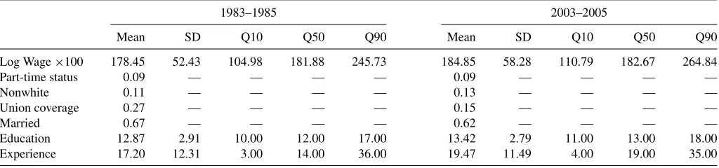
We use a dataset from Fortin, Lemieux, and Firpo (2011), which was extracted from the 1983–1985 and 2003–2005 Out-going Rotation Group (ORG) supplements of the CPS. See Lemieux (2006) for further details on its construction. Our data contain information on 232,784 and 170,693 males, re-spectively, that were employed in the relevant periods. Workers in the 1983–1985 and 2003–2005 sample play the role of our groups 0 and 1. The outcome variable of interest is the log hourly wage, measured in constant 1985 dollars and multiplied by 100 (to improve the readability of the tables below). The covariates are years of education, years of potential labor market experi-ence, and dummies for union coverage, race, marital status, and part-time status. All observations are weighted by the product of the number of hours worked and their respective CPS sample weights.
Some descriptive statistics are given in Table 1. Results on wages confirm the general picture that was found before in the literature. Over the sample period, the 90% quantile of the wage distribution has been rising substantially, while the 10% quantile and the median exhibit only a moderate increase or have remained approximately constant, respectively. There is thus a large increase in wage inequality as measured by the difference between the 90% and the 10% quantile, but this is the effect of an increase in inequality in the right tail of the distribution. Regarding the covariates, the most striking fea-ture is certainly the decline in union coverage from 27% in 1983–1985 to only 15% in 2003–2005. The average (poten-tial) labor market experience and the average years of education both increased substantially by more than 2 years and 6 months, respectively. Changes in other explanatory variables are less pronounced.
To estimate the various elements of our decomposition of the composition effect, we proceed as described in Section 5. We model the copula functionsCg by a Gaussian copula, and
the conditional CDFsFYg|Xby a distributional regression model with a Gaussian link function. Compared to an approach based on quantile regression, distributional regression has the advan-tage that it is not affected by heaping in the distribution of wages, and seems to be better suited to capture the somewhat irregular behavior of the conditional wage distribution around the level of the minimum wage (Chernozhukov, Fernandez-Val,
Table 1. Descriptive statistics
1983–1985 2003–2005
Mean SD Q10 Q50 Q90 Mean SD Q10 Q50 Q90
Log Wage×100 178.45 52.43 104.98 181.88 245.73 184.85 58.28 110.79 182.67 264.84
Part-time status 0.09 — — — — 0.09 — — — —
Nonwhite 0.11 — — — — 0.13 — — — —
Union coverage 0.27 — — — — 0.15 — — — —
Married 0.67 — — — — 0.62 — — — —
Education 12.87 2.91 10.00 12.00 17.00 13.42 2.79 11.00 13.00 18.00
Experience 17.20 12.31 3.00 14.00 36.00 19.47 11.49 4.00 19.00 35.00
and Melly2013; Rothe and Wied2013). In addition to the co-variates mentioned above, we use quadratic terms in education and experience and a full set of interaction terms for estimat-ing the conditional CDFs. Standard errors are calculated via the nonparametric bootstrap, using B=200 replications. Due to the large sample sizes, sampling variation in our estimates is mostly negligible.
Tables 2and3 present the results of our decomposition for various measures of location and spread, respectively. Row by row, we report estimates of the total change ν
O, the usual
structure and composition effectνS andνX, our dependence and marginal distribution effectsνD andνM, the direct con-tributions νM(el) for each of the six covariates, and
“two-way” interaction terms νM(k) with |k| =2. For brevity, we
do not report estimates higher-order interactions. Estimates of the total changeνO, which impose the parametric restrictions on copulas and conditional distribution functions as explained above, are very close to the respective descriptive statistics that can be calculated directly fromTable 1. We take this as an assuring indication that our parametric model provides a reasonable fit.
We first consider estimates of the structure and composi-tion effect, which are both parameters that could also be esti-mated via other methods (e.g., DiNardo, Fortin, and Lemieux 1996; Machado and Mata 2005; Rothe 2010; Chernozhukov, Fernandez-Val, and Melly2013, among many others).Table 2 shows that changes in labor force composition alone can explain a substantial part of the total change in the mean wage, but they do not offer an explanation for the differential change at various quantiles. For example, the estimates suggest that changes in labor force composition alone would have led to a large upward shift of the median wage, while the total observed change be-tween 1985 and 2005 was in fact close to zero. We can also see fromTable 2that the composition effect is positive for each of the three quantiles under consideration, with the magnitude of the effect gradually increasing with the quantile level. Corre-spondingly, the composition effect amount to about two-thirds of the increase in the 90%–10% quantile differences, but has the opposite sign of the total change in the 50%–10% quantile differences.
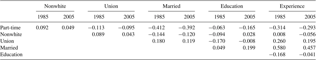
We now consider the estimates of the further decomposition proposed in this article, starting with the dependence effect. To interpret this component, it is important to understand the changes in the dependence structure of the covariates that took
place over the study period. To that end,Table 4reports estimates of the copula parameters from the 1985 and 2005 samples, respectively (recall that we are working with a Gaussian copula that is parameterized through a correlation matrix).
The point estimates show several interesting developments. For example, negative associations between union coverage and education as well as being nonwhite and education essen-tially vanished over the study period. Working part-time became more negatively associated with education. Being married be-came more strongly associated with education, and somewhat less strongly with experience. The dependence effect measures the joint contribution of these changes. FromTable 3, we can see that it plays a substantial role for the various measures of spread, explaining about 25% of the respective composi-tion effects. In case of the 10% quantile, the dependence ef-fect is of roughly the same absolute magnitude as the com-position effect but has the opposite sign. For the other mea-sures of location inTable 2, the dependence effect is relatively small.
Next, we consider the “direct” marginal distribution effects and “two-way” interaction effects of the six explanatory vari-ables. FromTable 2, we find that changes in the distribution of education and experience both have a similar, strongly positive “direct” impact on all quantiles, with slightly larger magnitudes for the median relative to the two extreme quantiles. That is, our estimates suggested that a counterfactual change in the marginal distribution of either education or experience to its respective 2005 value would have shifted the 1985 wage distribution to the right, while otherwise approximately preserving its overall shape. Correspondingly,Table 3shows that changes in educa-tion or experience alone contribute only moderately to the total increase in inequality observed over that period. Moreover, we see fromTable 2that these two variables have a sizable negative interaction effect on the median, and a positive interaction effect of similar absolute magnitude on the 10% quantile. As a con-sequence, we also observe corresponding nonzero interaction terms for the various quantile differences inTable 3. To better understand the interpretation of the interaction effects, consider the case of the median. Our estimates suggest that a counter-factual change in the marginal distribution ofbotheducation or experience to its respective 2005 value (while holding every-thing else constant) would have increased the 1985 median by the sum of the two direct contributions and the corresponding interaction term, that is, by 5.631+5.629−0.966=10.294.
Table 2. Estimated decomposition of differences in distribution of log hourly wages (×100) of workers in 2003–2005 and 1983–1985 using CPS data
Mean Q90 Q50 Q10
Total differenceν
O 6.479 (0.189) 18.756 (0.327) 0.862 (0.289) 5.401 (0.267)
Structure effectν
S 1.007 (0.167) 8.398 (0.338) −5.632 (0.308) 3.660 (0.272)
Composition effectν
X 5.472 (0.127) 10.358 (0.190) 6.493 (0.217) 1.742 (0.183)
Dependence effectν
D −0.382 (0.033) 0.737 (0.063) −0.448 (0.063) −1.647 (0.096)
Marginal distr. effectν
M 5.854 (0.121) 9.621 (0.171) 6.941 (0.211) 3.388 (0.181)
“Direct” contribution to composition effect (ν M(e
j))
Part-time −0.051 (0.013) 0.016 (0.004) −0.045 (0.012) −0.143 (0.038)
Nonwhite −0.263 (0.018) −0.191 (0.016) −0.329 (0.026) −0.265 (0.021)
Union coverage −2.327 (0.035) 1.092 (0.058) −3.913 (0.085) −2.636 (0.093)
Married −0.526 (0.019) −0.254 (0.019) −0.634 (0.035) −0.640 (0.034)
Education 4.349 (0.074) 4.112 (0.104) 5.631 (0.138) 4.005 (0.126)
Experience 4.307 (0.058) 4.468 (0.100) 5.629 (0.121) 3.647 (0.112)
“Two-way” interactions (ν
M(k) with|k| =2)
Part-time:Nonwhite 0.000 (0.000) −0.001 (0.000) −0.001 (0.003) 0.001 (0.005)
Part-time:Union coverage −0.007 (0.002) −0.005 (0.002) −0.007 (0.004) −0.019 (0.011)
Part-time:Married −0.001 (0.000) −0.001 (0.000) −0.001 (0.004) −0.011 (0.008)
Part-time:Education −0.001 (0.000) 0.001 (0.002) −0.003 (0.003) −0.037 (0.019)
Part-time:Experience 0.003 (0.001) 0.003 (0.003) 0.001 (0.004) −0.028 (0.018)
Nonwhite:Union coverage −0.014 (0.002) −0.004 (0.006) −0.001 (0.018) −0.038 (0.018)
Nonwhite:Married 0.003 (0.000) −0.001 (0.002) 0.001 (0.012) −0.024 (0.013)
Nonwhite:Education 0.004 (0.001) 0.018 (0.008) −0.005 (0.018) −0.069 (0.020)
Nonwhite:Experience −0.015 (0.001) 0.009 (0.008) −0.046 (0.017) −0.080 (0.020)
Union coverage:Married −0.035 (0.003) −0.022 (0.006) −0.030 (0.032) −0.070 (0.046)
Union coverage:Education 0.315 (0.009) 0.241 (0.058) 0.265 (0.122) −0.245 (0.105)
Union coverage:Experience 0.084 (0.007) 0.165 (0.053) −0.158 (0.069) −0.303 (0.108)
Married:Education 0.002 (0.003) 0.013 (0.015) 0.027 (0.022) −0.169 (0.043)
Married:Experience −0.013 (0.004) 0.013 (0.012) −0.001 (0.032) −0.188 (0.041)
Education:Experience 0.016 (0.006) −0.094 (0.102) −0.966 (0.146) 0.911 (0.138)
NOTE: Bootstrapped standard errors (200 replications) are in parenthesis.
333
Table 3. Estimated decomposition of differences in distribution of log hourly wages (×100) of workers in 2003–2005 and 1983–1985 using CPS data
Std. Dev. Q90-10 Q90-50 Q50-10
Total differenceν
O 5.984 (0.118) 13.355 (0.387) 17.895 (0.352) −4.540 (0.316)
Structure effectν
S 3.456 (0.126) 4.738 (0.421) 14.030 (0.392) −9.291 (0.373)
Composition effectν
X 2.528 (0.062) 8.616 (0.234) 3.865 (0.237) 4.752 (0.192)
Dependence effectν
D 0.681 (0.030) 2.384 (0.119) 1.185 (0.074) 1.199 (0.105)
Marginal distr. effectν
M 1.847 (0.050) 6.232 (0.217) 2.680 (0.226) 3.553 (0.194)
“Direct” contribution to composition effect (ν M(ej))
Part-time 0.052 (0.014) 0.159 (0.042) 0.061 (0.016) 0.099 (0.026)
Nonwhite 0.037 (0.004) 0.073 (0.015) 0.137 (0.018) −0.064 (0.018)
Union coverage 1.153 (0.021) 3.728 (0.112) 5.006 (0.105) −1.278 (0.105)
Married 0.184 (0.009) 0.386 (0.034) 0.380 (0.036) 0.006 (0.035)
Education −0.050 (0.023) −0.107 (0.138) −1.518 (0.134) 1.625 (0.147)
Experience 0.156 (0.026) 0.821 (0.136) −1.162 (0.141) 1.982 (0.146)
“Two-way” interactions (ν
M(k) with|k| =2)
Part-time:Nonwhite −0.001 (0.000) −0.002 (0.001) −0.001 (0.003) −0.002 (0.006)
Part-time:Union coverage −0.001 (0.001) 0.012 (0.011) 0.001 (0.002) 0.011 (0.011)
Part-time:Married 0.000 (0.000) −0.001 (0.003) 0.001 (0.003) −0.003 (0.005)
Part-time:Education 0.003 (0.001) 0.043 (0.015) −0.003 (0.003) 0.046 (0.016)
Part-time:Experience 0.004 (0.001) 0.036 (0.013) −0.001 (0.003) 0.037 (0.014)
Nonwhite:Union coverage −0.002 (0.001) 0.040 (0.019) 0.005 (0.020) 0.035 (0.025)
Nonwhite:Married −0.002 (0.001) −0.003 (0.010) −0.026 (0.021) 0.023 (0.024)
Nonwhite:Education 0.005 (0.001) 0.092 (0.019) 0.026 (0.018) 0.065 (0.024)
Nonwhite:Experience 0.009 (0.001) 0.097 (0.020) 0.052 (0.020) 0.045 (0.024)
Union coverage:Married −0.007 (0.002) 0.057 (0.047) 0.014 (0.042) 0.042 (0.055)
Union coverage:Education 0.142 (0.005) 0.486 (0.121) −0.024 (0.139) 0.510 (0.156)
Union coverage:Experience 0.174 (0.005) 0.514 (0.114) 0.312 (0.139) 0.202 (0.153)
Married:Education 0.013 (0.002) 0.185 (0.041) −0.026 (0.034) 0.211 (0.052)
Married:Experience 0.022 (0.003) 0.201 (0.043) 0.011 (0.035) 0.189 (0.053)
Education:Experience −0.036 (0.005) −1.005 (0.170) 0.872 (0.178) −1.877 (0.148)
NOTE: Bootstrapped standard errors (200 replications) are in parenthesis.
334
Table 4. Estimated copula parameters
Nonwhite Union Married Education Experience
1985 2005 1985 2005 1985 2005 1985 2005 1985 2005
Part-time 0.092 0.049 −0.113 −0.095 −0.412 −0.392 −0.063 −0.165 −0.314 −0.293
Nonwhite 0.089 0.043 −0.144 −0.120 −0.094 0.028 0.008 −0.056
Union 0.180 0.119 −0.170 −0.008 0.260 0.195
Married 0.049 0.199 0.580 0.457
Education −0.168 −0.041
NOTE: Estimates of the parameters of the Gaussian copula, which determine the pairwise dependence structure between the two respective covariates.
The results also suggest that the decline in unionization had an important impact on the distribution of wages. Changes in union coverage rates are estimated to have a strong negative effect on the median wage, a somewhat less negative one on the 10% quantile, and a small positive effect on the 90% quantile. This covariate is thus the single most important one for explaining changes in overall and top-end inequality, as it accounts for about 25% of the observed change in each the 90%–10% and 90%–50% quantile differences alone. There are also some minor interactions between union coverage and both education and experience.
Finally, our estimates suggest that changes in the proportion of part-time, nonwhite, and married workers are of compara-tively minor importance relative to the aforementioned covari-ates when it comes to explaining the composition effect. This comes as no surprise asTable 1shows that the marginal dis-tribution of these variables did not change much between 1985 and 2005.
8. CONCLUSIONS
Studying the role of specific covariates in determining between-group differences in economic outcomes involves a number of subtle yet important issues. Using results from cop-ula theory, we show that the composition effect naturally has an interesting structure that can be exploited in empirical ap-plications. In particular, we show that the composition effect can be written as the sum of three types of components: (i) the “direct contribution” of each covariate due to between-group differences in the respective marginal distributions, (ii) several “two-way” and “higher-order interaction effects” due to the in-terplay between two or more marginal distributions, and (iii) a “dependence effect” accounting for different dependence pat-terns among the covariates. We show how these components can be estimated using flexible parametric specifications, and illus-trate the procedure through an application to U.S. wage data. The empirical application suggests that our method is able to uncover new and interesting features of the data, which have thus far not been detected by other approaches.
APPENDIX A: PROOF OF ASYMPTOTIC PROPERTIES
In this section, we formally prove the asymptotic normality result given in Section6. For notational simplicity, suppose thatn1=n0≡
n∗, which means that we can work withλ1=λ0=1/2. As a first step,
Using Assumptions 2–3 and the Glivenko–Cantelli Theorem, it follows that
Using Assumptions 3–4 and the Glivenko–Cantelli Theorem, it follows that
uniformly overy. Finally, the termT4can be written as
T4=