Full Terms & Conditions of access and use can be found at
http://www.tandfonline.com/action/journalInformation?journalCode=ubes20
Download by: [Universitas Maritim Raja Ali Haji] Date: 12 January 2016, At: 00:23
Journal of Business & Economic Statistics
ISSN: 0735-0015 (Print) 1537-2707 (Online) Journal homepage: http://www.tandfonline.com/loi/ubes20
Default Estimation and Expert Information
Nicholas M. Kiefer
To cite this article: Nicholas M. Kiefer (2010) Default Estimation and Expert Information, Journal of Business & Economic Statistics, 28:2, 320-328, DOI: 10.1198/jbes.2009.07236 To link to this article: http://dx.doi.org/10.1198/jbes.2009.07236
Published online: 01 Jan 2012.
Submit your article to this journal
Article views: 137
View related articles
Default Estimation and Expert Information
Nicholas M. K
IEFERDepartments of Economics and Statistical Science and Center for Analytic Economics, Cornell University, 490 Uris Hall, Ithaca, NY 14853-7601, Risk Analysis Division, Office of the Comptroller of the Currency, U.S. Department of the Treasury, and CREATES (nicholas.kiefer@cornell.edu)
Default is a rare event, even in segments in the midrange of a bank’s portfolio. Inference about default rates is essential for risk management and for compliance with the requirements of Basel II. Most com-mercial loans are in the middle-risk categories and are to unrated companies. Expert information is crucial in inference about defaults. A Bayesian approach is proposed and illustrated using a prior distribution as-sessed from an industry expert. The binomial model, most common in applications, is extended to allow correlated defaults. A check of robustness is illustrated with anǫ-mixture of priors.
KEY WORDS: Basel II; Bayesian inference; Correlated defaults; Prior assessment; Risk management; Robustness.
1. INTRODUCTION
Estimation of default probabilities (PD), loss given default (LGD, a fraction), and exposure at default (EAD) for portfo-lio segments containing reasonably homogeneous assets is es-sential to prudent risk management. It is also crucial for com-pliance with Basel II (B2) rules for banks using the IRB ap-proach to determine capital requirements (Basel Committee on Banking Supervision 2004). Estimation of small probabilities is tricky, and this article will focus on estimating PD. The em-phasis is on segments in the middle of the risk profile of the portfolio. Although the risk is in the middle of the asset mix, the probability of default is still “small.” It is, in fact, likely to be about 0.01; defaults, though seen, are rare. The bulk of a typical bank’s commercial loans are concentrated in these seg-ments (segseg-ments differ across banks). Very low risk institutions are relatively few in number and they have access to capital through many avenues in addition to commercial loans. Very high risk loans are largely avoided and when present are often due to the reclassification of a safer loan as conditions change. To put this in perspective, the middle-quality loans are approxi-mately S&P Baa or Moody’s BBB. In practice the bulk of these loans are to unrated companies and the bank has done its own rating to assign the loans to risk “buckets.” The focus of this article is on estimation of the default probability for such a risk bucket on the basis of historical information and expert knowl-edge.
Throughout the article we take a probability approach to the quantitative description of uncertainty. There are many argu-ments that uncertainty is best described in terms of probabili-ties. The classic axiomatic treatment isSavage(1954). In the case of default modeling, where measuring and controlling risk is the aim, it is natural to focus on anticipating defaults, or at least anticipating the aggregate number of defaults. Suppose there are a number of default configurations, and we wish to assign numbers to these events and to use these numbers to de-scribe the likelihood of the events. Simple arguments based on scoring rules (for example minimizing squared prediction er-ror) or odds posting (avoiding certain losses) imply that these numbers must combine like probabilities. For constructions see
De Finetti (1974). Lindley (1982b) elaborated on the devel-opment using scoring rules, Heath and Sudderth (1978) and
Berger(1980) on betting. Reasoning about probabilities is not easy. There is a long literature beginning withKahneman and Tversky(1974) demonstrating that people, in practice, find it difficult to think about probabilities consistently. Theoretical alternatives to probabilistic reasoning include possibility mea-sures, plausibility meamea-sures, etc. These are reviewed and eval-uated by Halpern (2003). Although these practical and theo-retical objections to probability are often used to criticize the Bayesian approach, they apply equally to the likelihood speci-fication and the modeling approach to risk management. While recognizing these objections, this article will use the probability approach, noting that alternatives invariably lead to incoherence (De Finetti 1974).
2. A STATISTICAL MODEL FOR DEFAULTS
The simplest and most common probability model for de-faults of assets in a homogeneous segment of a portfolio is the binomial, in which the defaults are independent across assets and over time, and defaults occur with common probabilityθ. This is the most widely used specification in practice and may be consistent with B2 requirements calling for a long-run aver-age default probability. Note that specification of this model re-quires expert judgement, that is, information. Denote the expert information bye. The role of expert judgement is not usually explicitly indicated at this stage, so it is worthwhile to point to its contribution. First, consider the statistical model. The inde-pendent Bernoulli model is not the only possibility. Certainly independence is a strong assumption and would have to be con-sidered carefully. External factors not explicitly modeled, for example general economic conditions, could induce correla-tion. There is evidence that default probabilities vary over the business cycle (for example, Nickell, Perraudin, and Varotto 2000); we return to this topic below. The Basel prescription is for a marginal annual default probability, however, and corre-lation among defaults is accommodated separately in the for-mula for the capital requirement. Thus, many discussions of
© 2010American Statistical Association Journal of Business & Economic Statistics
April 2010, Vol. 28, No. 2 DOI:10.1198/jbes.2009.07236
320
Kiefer: Default Estimation and Expert Information 321
the inference issue have focussed on the binomial model and the associated frequency estimator. Second, are the observa-tions really identically distributed? Perhaps the default prob-abilities differ across assets, even within the group. Can this be modeled, perhaps on the basis of asset characteristics? The requirements demand an annual default probability, estimated over a sample long enough to cover a full cycle of economic conditions. Thus the probability should be marginal with re-spect to external conditions. For specificity we will continue with the binomial specification, but will turn attention below to an extension allowing correlated defaults (also possibly con-sistent with B2) below. Letdi indicate whether theith obser-vation was a default (di=1) or not (di=0). The Bernoulli model (a single binomial trial) for the distribution of di is
p(di|θ,e)=θdi(1−θ )1−di. Let D= {di,i=1, . . . ,n}denote the whole dataset andr=r(D)=idi the count of defaults. Then the joint distribution of the data is
p(D|θ,e)= As a function ofθ for given dataDthis is the likelihood func-tion L(θ|D,e).Since this distribution depends on the data D only throughr(nis regarded as fixed), the sufficiency principle implies that we can concentrate attention on the distribution of
r easy to underappreciate the simplification obtained by passing from Equation (1) to Equation (2). Instead of separate treatment for each of the 2ndatasets possible, it is sufficient to restrict at-tention ton+1 dataset types, characterized by the value ofr. This theory of types can be made the basis of a theory of as-ymptotic inference. SeeCover and Thomas(1991). In our ap-plication, the set of likely values ofris small, and an analysis can be done for each of these values of r, rather than for the
n r
distinct datasets corresponding to each value ofr. Thus, by analyzing a few likely dataset types, we analyze, in effect, all of the most likely data realizations.
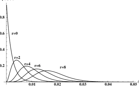
Regarded as a function ofθ for fixedr, Equation (2) is the likelihood function. Figure1shows the likelihood functions for
n=500, a reference dataset size, andr= {0,2,4,6,8}.
3. UNCERTAIN DEFAULT PROBABILITIES
Equation (2) is a statistical model. It generates probabilities for all default configurations as a function of a single parame-terθwhich remains unspecified. The default probabilityθis an unknown, but that does not mean that nothing is known about its value. In fact, defaults are widely studied and risk managers, modelers, validators, and supervisors have detailed knowledge on values ofθ for particular portfolio segments. The point is thatθ is unknown in the same sense that the future default sta-tus of a particular asset is unknown. The fact that default is in the future is not important; the key is that it is unknown and the uncertainty can be described and quantified. We have seen
Figure 1. Likelihood functionsn=500.
how uncertain defaults can be modeled. The same methods can be used to model the uncertainty aboutθ.Continuing with the logic used to model default uncertainty, we see that uncertainty about values ofθare coherently described by probabilities. We assemble these probability assessments into a distribution de-scribing the uncertainty aboutθgiven the expert informatione,
p(θ|e).
The distributionp(θ|e)can be a quite general specification, reflecting, in general, the assessments of uncertainty in an infin-ity of possible events. This is in contrast with the case of default configurations, in which there are only a finite (though usually large) number of possible default configurations. However, this should not present an insurmountable problem. Note that we are quite willing to model the large number of probabilities as-sociated with the possible different default configurations with a simple statistical model—the binomial. The same approach is taken for the prior specification. That is, we can fit a few prob-ability assessments by an expert to a suitable functional form and use that distribution to model prior uncertainty. There is some approximation involved, and care is necessary. In this re-gard, the situation is no different from that present in likelihood specification.
A convenient functional form is the beta distribution
p(θ|α, β)= Ŵ(α+β)
Ŵ(α)Ŵ(β)θ
α−1(
1−θ )β−1, (3)
which has mean α/(α+β) and variance αβ/((α+β)2(1+
α+β)). A particularly easy generalization is to specify the supportθ∈ [a,b] ⊂ [0,1].It is possible that some applications would require the support ofθto consist of the union of disjoint subsets of[0,1],but this seems fanciful in the current applica-tion. Let t have the beta distribution and change variables to
θ (t)=a+(b−a)twith inverse functiont(θ )=(θ−a)/(b−a) flexibility within the range[a,b], but in some situations it may be too restrictive. For example it may not be flexible enough to
allow combination of information from many experts. A simple generalization is the 7-parameter mixture of two 4-parameter betas with common support. Computations with this mixture distribution are not substantially more complicated than compu-tations with the 4-parameter beta alone. If necessary, more mix-ture components with new parameters can be added, although it seems unlikely that expert information would be detailed and specific enough to require this complicated a representa-tion. A useful further generalization is given by the 9-parameter mixture allowing different supports for the two mixture com-ponents. By choosing enough beta-mixture terms the approxi-mation of an arbitrary continuous priorp(θ|e)for a Bernoulli parameter can be made arbitrarily accurate, in the sense that the sequence of approximations can be chosen to converge uni-formly top(θ|e).Note that there is nothing stochastic in this ar-gument. The proof follows the proof of the Stone–Weierstrass approximation theorem for approximation of continuous func-tions by polynomials. SeeDiaconis and Ylvisaker(1985). The use of mixtures in simulating posterior densities is advocated byHoogerheide, Kaashoek, and van Dijk(2007).
4. INFERENCE
With the likelihood and prior at hand inference is a straight-forward application of Bayes’ rule. Given the distribution
p(θ|e),we obtain the joint distribution ofr, the number of de-faults, andθ:
p(r, θ|e)=p(r|θ,e)p(θ|e),
from which we obtain the marginal (predictive) distribution ofr,
p(r|e)=
p(r, θ|e)dθ. (5) If the value of the parameterθ is of main interest we divide to obtain the conditional (posterior) distribution ofθ:
p(θ|r,e)=p(r|θ,e)p(θ|e)/p(r|e), (6) which is Bayes’ rule. Since Basel II places more emphasis on the default probability than on the number of defaults in a given portfolio segment, we focus our discussion onp(θ|r,e). Note as an aside that if defaults are a sample from an infinite exchange-able sequence then the marginal distribution of the number of defaults can always be written as a binomial mixture, so the parametric specification may not be as restrictive as it seems. SeeDe Finetti(1974).
5. PRIOR DISTRIBUTION
I asked an expert to specify a portfolio and to give me some aspects of his beliefs about the unknown default probability. The portfolio consists of loans that might be in the middle of a bank’s portfolio. These are typically commercial loans, mostly to unrated companies. If rated, these might be about S&P Baa or Moody’s BBB. The method included a specification of the problem and some specific questions followed by a discussion. General discussions of the elicitation of prior distributions were given byKadane et al.(1980),Kadane and Wolfson(1998), and
Garthwaite, Kadane, and O’Hagan(2005). An example assess-ing a prior for a Bernoulli parameter isChaloner and Duncan
(1983). Chaloner and Duncan followed Kadane et al. in sug-gesting that assessments be done not directly on the probabil-ities concerning the parameters, but on the predictive distrib-ution. That is, questions should be asked about observables, to bring the expert’s thoughts closer to familiar ground. In the case of a Bernoulli parameter and a 2-parameter beta prior, Chaloner and Duncan suggested first eliciting the mode of the predictive distribution for a givenn(an integer), then assessing the rela-tive probability of the adjacent values (“dropoffs”). Graphical feedback is provided for refinement of the specification. Ex-amples considern=20.Gavasakar(1988) suggested an alter-native method, based on assessing modes of predictive distri-butions but not on dropoffs. Instead, changes in the mode in response to hypothetical samples are elicited and an explicit model of elicitation errors is proposed. The method is evaluated in then=20 case and appears competitive. The suggestion to interrogate experts on what they would expect to see in data, rather than what they would expect of parameter values, is ap-pealing and I have, to some extent, pursued this with our expert. This approach may be less attractive in the case of large sample sizes and small probabilities, and in our particular application, where the expert was sophisticated about probabilities. Our ex-pert found it easier to think in terms of the probabilities directly than in terms of defaults in a hypothetical sample.
Thinking about uncertainty in terms of probabilities requires effort and practice (possibly explaining why it is so rarely done). Nevertheless it can be done once experts are convinced it is worthwhile. Indeed, there is experimental evidence in game settings that elicited beliefs about opponents’ future actions are better explanations of responses than empirical beliefs— Cournot or fictitious play—based on weighted averages of pre-vious actions. For details seeNyarko and Schotter(2002).
The precise definition of default is at issue. In the eco-nomic theory of the firm, default occurs when debt payments are missed and ownership and control of the firm passes from existing owners (shareholders in the case of a corporation) to debtholders. As a lesser criterion, loans that are assigned to “nonaccrual” may be considered defaulted. We simply note the importance of using consistent definitions in the assessment of expert information and in data definition.
We did the elicitation first assuming a sample of 500 asset-years. For our application, we also considered a “small” sample of 100 observations and a “large” sample of 1000 observations, and occasionally an enormous sample of 10,000 observations. Considering first the predictive distribution on 500 observa-tions, the modal value was five defaults. Upon being asked to consider the relative probabilities of four or five defaults, condi-tional on four or five defaults occurring (the conditioning does not matter here, for the probability ratio, but it is thought to be easier to think about when posed in this fashion), the expert ex-pressed some trepidation as it is difficult to think about such rare events. Ultimately, the expert gave probability ratios not achievable by the binomial model even with known probability. This experience supports the implication ofGavasakar(1988) that dropoff probabilities are problematic. The expert was quite happy in thinking about probabilities over probabilities how-ever. This may not be so uncommon in this technical area, as
Kiefer: Default Estimation and Expert Information 323
practitioners are accustomed to working with probabilities. The mean value was 0.01. The minimum value for the default prob-ability was 0.0001 (one basis point). The expert reported that a value above 0.035 would occur with probability less than 10%, and an absolute upper bound was 0.3. The upper bound was dis-cussed: the expert thought probabilities in the upper tail of his distribution were extremely unlikely, but he did not want to rule out the possibility that the rates were much higher than antici-pated (prudence?). Quartiles were assessed by asking the expert to consider the value at which larger or smaller values would be equiprobable given the value was less than the median, then given the value was more than the median. The median value was 0.01. The former was 0.0075. The latter, the 0.75 quar-tile, was assessed at 0.0125. The expert seemed to be thinking in terms of a normal distribution, perhaps using, informally, a central limit theorem combined with long experience with this category of assets.
This set of answers is more than enough information to de-termine a 4-parameter beta distribution. I used a method of mo-ments to fit parametric probability statemo-ments to the expert as-sessments. The moments I used were squared differences rela-tive to the target values, for example((a−0.0001)/0.0001)2. The support points were quite well-determined for a range of {α, β}pairs at the assessed values{a,b} = [0.0001,0.3]. These were allowed to vary (the parameter set is overdetermined), but the optimization routine did not change them beyond the sev-enth decimal place. Thus, the expert was able to determine these parameter values consistently with his probability assessments. Further, changing the weights did not matter much either. Prob-ably this is due to the fact that there is almost no probability in the upper tail, so changing the upper bound made almost no difference in the assessed probabilities. Thus the rather high (?) value ofb reflects the long tail apparently desired by the ex-pert. The {α, β} parameters were rather less well-determined (the sum of squares function was fairly flat) and I settled on the values (7.9, 224.8) as best describing the expert’s information. The resulting prior distributionp(θ|e)has virtually no proba-bility on the long right-tail. A closeup view of the relevant part of the prior is graphed in Figure2.
The median of this distribution is 0.00988, the mean is 0.0103, and the standard deviation is 0.00355. In practice, after the information is aggregated into an estimated probability dis-tribution, then additional properties of the distribution would
Figure 2. Expert information: closeup.
Figure 3. Predictive distributionp(r|e).
be calculated and the expert would be consulted again to see if any changes were in order before proceeding to data analy-sisLindley(1982a). This process would be repeated as neces-sary. In the present application there was one round of feedback, valuable since the expert had had time to consider the probabil-ities involved. The characteristics reported are from the second round of elicitation. An application within a bank might do ad-ditional rounds with the expert, or consider alternative experts and a combined prior.
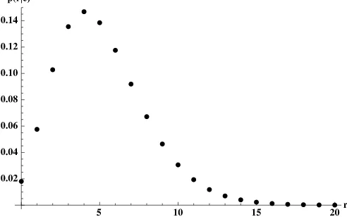
The predictive distribution in Equation (5) corresponding to this prior is given in Figure3forn=500.
With our specification, the expected value of r,E(r|e)= n
k=0kp(k|e)is 5.1 forn=500. Total defaults numbering zero through nine characterize 92% of expected datasets. Thus, car-rying out our analysis for these 10 data types, comprising about 262 distinct datasets, a trivial fraction of the 2500 pos-sible datasets, actually covers 92% of the expected realizations. Defaults are expected to be rare events. Thus we are not analyz-ing one particular dataset, rather we provide results applicable to 92% of the likely datasets.
6. POSTERIOR ANALYSIS
The posterior distribution, p(θ|r,e), is graphed in Figure4
forr=0, 2, 4, 6, and 8, andn=500. The corresponding likeli-hood functions, for comparison, were given in Figure1. Note
Figure 4. Posterior densitiesp(θ|r,e).
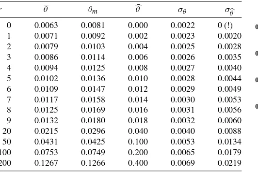
Table 1. Default probabilities—location and precision,n=500
r θ θm θ σθ σθ
0 0.0063 0.0081 0.000 0.0022 0 (!) 1 0.0071 0.0092 0.002 0.0023 0.0020 2 0.0079 0.0103 0.004 0.0025 0.0028 3 0.0086 0.0114 0.006 0.0026 0.0035 4 0.0094 0.0125 0.008 0.0027 0.0040 5 0.0102 0.0136 0.010 0.0028 0.0044 6 0.0109 0.0147 0.012 0.0029 0.0049 7 0.0117 0.0158 0.014 0.0030 0.0053 8 0.0125 0.0169 0.016 0.0031 0.0056 9 0.0132 0.0180 0.018 0.0032 0.0060 20 0.0215 0.0296 0.040 0.0040 0.0088 50 0.0431 0.0425 0.100 0.0053 0.0134 100 0.0753 0.0749 0.200 0.0065 0.0179 200 0.1267 0.1266 0.400 0.0069 0.0219
the substantial differences in location. Comparison with the likelihood functions graphed in Figure1and the prior distribu-tion graphed in Figure2reveals that the expert provides much more information to the analysis than do the data.
Given the distributionp(θ|r,e), we might ask for a summary statistic, a suitable estimator for plugging into the required cap-ital formulas as envisioned by Basel Committee on Banking Supervision(2004). A natural value to use is the posterior ex-pectation,θ=E(θ|r,e).The expectation is an optimal estimator under quadratic loss and is asymptotically an optimal estimator under bowl-shaped loss functions (use the Bernstein–von Mises theorem on convergence of the posterior to a normal distribu-tion and Anderson’s lemma on minimum loss, van der Vaart 1998, theorem 10.1 and lemma 8.5). An alternative, by analogy with the maximum likelihood estimatorθ, is the posterior mode
θm. As a summary measure of our confidence we would use the posterior standard deviationσθ=
E(θ−θ2).By comparison, the usual approximation to the standard deviation of the maxi-mum likelihood estimator isσθ=θ (1−θ )/n.These quanti-ties are given in Table1for r=0–9 andr=20,50,100,200. As noted, ther=0–9 case covers the 262 most likely datasets out of the possible 2500. Together, these comprise analyses of 92% of likely datasets. The r=20 case is an extremely low probability outcome—less than 0.0001—and is included to show the results in this case. There are approximately 2118 datasets corresponding tor=20. The rows forr=50,100, and 200 are included as a further “stress test” and will be discussed below. Their combined prior probability of occurrence is less than 10−14.
For values ofrbelow its expected value the posterior mean is greater than the MLE, for values above the posterior is less than the MLE, as expected. As is well-known and widely discussed, the MLE is unsatisfactory when there are no observed defaults (Basel Committee on Banking Supervision 2005;BBA, LIBA, and ISDA 2005; Pluto and Tasche 2005; Kiefer 2008). The Bayesian approach provides a coherent resolution of the infer-ence problem without resorting to desperation (sudden reclas-sification of defaulted assets, technical gimmicks).
Expert information will have larger weight in smaller sample sizes, and smaller relative weight for larger sample sizes. For
n=1000, for example,r=5–15 reflects 76% of the most likely
Figure 5. Eθand MLEθforn=1000.
datasets;r=0–20 represents 97%. To put this in perspective, the casesr=0–20 correspond to approximately 2138 datasets out of a possible 21000.Thus, 97% of the likely observations are contained in the small fraction 2−862of the possible datasets, or 0.0021 of the possible types. A substantial simplification results from concentrating on the distribution of the sufficient statistic and use of expert judgement to characterize possible samples. Naturally, this simplification depends critically on the use of expert judgement in specification of the likelihood function (our choice admits a sufficient statistic) and in specification of the prior distribution. Rather than resorting to extensive tabulation, we report results for 97% of likely samples in Figure5. The error bands, dotted for the MLE and dashed for the prior mean, are plus/minus one standard deviation.
7. ROBUSTNESS—THE CAUTIOUS BAYESIAN
Suppose we are rather less sure of our expert than he is of the default probability. Or, more politely, how can we assess just how important the tightly-held views of the expert are in determining our estimates? Table1gives one answer by com-paring the MLE and the posterior location measures. Another answer was proposed byKiefer(2008), who considered a less-certain expert with a prior with the same location but substan-tially higher variance than the actual expert. An alternative ap-proach, more formal and based on the literature on Bayesian robustness (Berger and Berliner 1986), is to mix the actual ex-pert’s prior with an alternative prior, and see exactly how seri-ously the inferences are affected by changes in the mixing pa-rameter.Berger and Berliner(1986), in fact, suggested mixing in a class of distributions, corresponding to different amounts or directions of uncertainty in the prior elicitation. In this spirit, we will mix the expert’s 4-parameter beta distribution with a uni-form distribution. Here, there are two clear possibilities. One is to mix with the uniform on[a,b], accepting the expert’s bounds but examining robustness to alpha and beta. The second is to mix with the uniform on[0,1], allowing all theoretically fea-sible values ofθ. We choose the latter approach. This is not a completely comfortable approach. Although the uniform is commonly interpreted as an uninformative prior, it in fact has a mean of 1/2, not a likely value for our default probability by any reasonable prior. An alternative might be to mix with a prior
Kiefer: Default Estimation and Expert Information 325
Table 2. Robustness—posterior means for mixture priors,n=500
r θ;ǫ=0.01 θ;ǫ=0.1 θ;ǫ=0.2 θ;ǫ=0.3 θ;ǫ=0.4
0 0.0063 0.0063 0.0062 0.0061 0.0061 1 0.0071 0.0071 0.0071 0.0071 0.0070 2 0.0079 0.079 0.0079 0.0079 0.0078 3 0.0086 0.0086 0.0086 0.0086 0.0086 4 0.0094 0.0094 0.0094 0.0094 0.0094 5 0.0102 0.0102 0.0102 0.0102 0.0102 6 0.0109 0.0109 0.0110 0.0110 0.0110 7 0.0117 0.0117 0.0117 0.0118 0.0118 8 0.0125 0.0125 0.0125 0.0125 0.0126 9 0.0132 0.0133 0.0133 0.0134 0.0134 20 0.0358 0.0358 0.0386 0.0398 0.0405 50 0.1016 0.1016 0.1016 0.1016 0.1016 100 0.2012 0.2012 0.2012 0.2012 0.2012 200 0.4004 0.4004 0.4004 0.4004 0.4004
with the same mean as our expert’s distribution, but maximum variance. We do not pursue this here. Our results suggest that it would not make much difference; the key is to mix in a distrib-ution with full support, so that likelihood surprises can appear. We choose to mix the expert’s prior with a uniform on all of [0,1]. This allows input from the likelihood if the likelihood happens to be concentrated aboveb(or belowa). The mixture distribution is
p(θ|e, ǫ)=(1−ǫ)p(θ|α, β,a,b)I(θ∈ [a,b])+ǫ (7) for θ ∈ [0,1]. The approach can be used whichever prior is specified, not just the 4-parameter beta. Our robust prior is in the 9-parameter mixture family consisting of our expert’s 4-parameter beta mixed with the 4-parameter beta with para-meters {α, β,a,b} = {1,1,0,1}and mixing parameter ǫ. Ta-ble 2 shows the posterior means for the mixture priors for
ǫ= {0.01,0.1,0.2,0.3,0.4}.
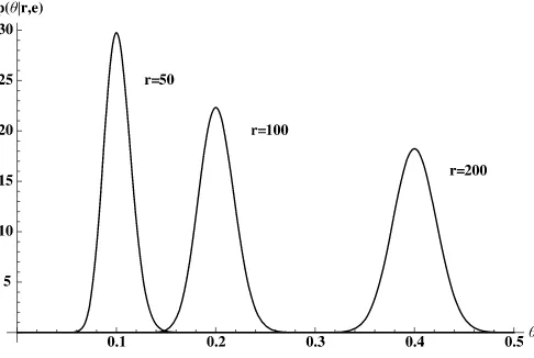
Mixing the expert’s prior with the uniform prior makes essen-tially no difference to the posterior mean for data in the likely part of the set of potential samples. Forr=20, unlikely but not outrageous, using the robust prior makes a substantial differ-ence. For the extremely unlikely values, 50, 100, 200, the dif-ferences are dramatic. The actual value ofǫ makes almost no difference. The numbers forǫ=0.001,not shown in the table, give virtually the same mean for all r. For comparison, we recall the values ofθ forr= {20,50,100,200}from Table1. These are{0.0215,0.0431,0.0753,0.1267}. Figure6shows the poste-rior distributions for our expert’s pposte-rior,p(θ|r,e)forr=50,100, and 200. It is clear that the prior plays a huge role here, as the likelihood mass is concentrated near 0.1, 0.2, and 0.4, while the prior gives only trivial weight to values greater than about 0.03, see Figures1 and2. On the other hand, Figure7shows the posterior corresponding to Equation (7) with 1% mixing (ǫ=0.01).Here, the likelihood dominates, as the likelihood value near the expert’s prior is vanishingly small relative to the likelihood in the tail area of the mixing prior.
Thus, the robust analysis with even a very small nonzero mix-ing fraction can reveal disagreements between the data and the expert opinion which are perhaps masked by the formal analy-sis. This robust analysis may have a role to play in the validation phase.
Figure 6. Posteriors withǫ=0,n=500.
In what sense is the robust analysis useful? We are really bringing something outside the model, namely the uniform dis-tribution representing no one’s beliefs, into the analysis as a for-mal tool for diagnostic analysis. The spirit is the same as usual procedures associated with good statistical practice–residual analysis, out of sample fits, forecast monitoring, or comparison with alternative models. All of these procedures involve step-ping away from the specified model and its analysis, and ask-ing, post estimation, does the specification make sense? Post es-timation model evaluation techniques are often informal, some-times problem specific, and require sound statistical judgement
OCC(2006). The analysis of robustness via an artificial prior is an attempt to merge the formal analysis with the informal post estimation model checking. A related method, checking for ir-relevant data using a mixture distribution, proposed by Ritov
(1985), might have a role as well.
8. HETEROGENEITY
It is clearly contemplated in the Basel II guidance that hetero-geneity is mitigated by the classification of assets into homo-geneous groups before estimation of the group-specific default probability. However, there may be remaining heterogeneity, due to systematic temporal changes in asset characteristics or to changing macroeconomic conditions. For fairly low-default
Figure 7. Posteriors withǫ=0.01,n=500.
portfolios there are unlikely to be enough data to sort out dif-ferences between years. However, there is evidence from other markets that default probabilities vary over the cycle, see for exampleNickell, Perraudin, and Varotto(2000). The B2 capi-tal requirements are based on a one-factor model due toGordy
(2003) that accommodates systematic temporal variation in as-set values and hence in default probabilities. This model can be used as the basis of a model that allows temporal variation in the default probabilities, and hence correlated defaults within years. The value of theith asset in timetis
vit=ρ1/2xt+(1−ρ)1/2ǫit,
where ǫit is the time and asset specific shock and xt is the common time shock, inducing correlation ρ across asset val-ues within a period. The random variables are assumed to be standard normal and independent. A mean of zero is attain-able through translation without loss of generality since we are only interested in default probabilities. Suppose default occurs ifvit<d,a default threshold value. The overall or marginal de-fault rate we are interested in is θ= (d).However, in each period the default rate depends on the realization of the system-atic factorxt; denote this θt.The model implies a distribution for θt.Specifically, the distribution of vit conditional onxt is N(ρ1/2xt,1−ρ).Hence the periodtdefault probability is
Thus forρ=0 there is random variation in the default proba-bility over time and this induces correlation in defaults across assets within a period. The distribution is given by
Pr(θt≤A)=Pr pert judgementeis quite clear. The parameters areθ,the mar-ginal or mean default probability, for which we have already assessed a prior, and the asset correlationρ.Values forρ are in fact prescribed inBasel Committee on Banking Supervision
(2006) for different asset classes. First, we defer to the B2 for-mulas and setρto a prescribed value (0.20) and dropρfrom the notation. Then, we consider the effect of generalizing this spec-ification. Moving toward the posterior forθ in this new speci-fication we note that the conditional distribution of the number of defaults in each period is [from Equation (2)]
p(rt|θt,e)=
from which we obtain the distribution conditional on the para-meter of interest
θfor fixedR, Equation (8) is the likelihood function. With this
Figure 8. Posterior with heterogeneity.
in hand we can calculate the posterior distribution using Equa-tions (5) and (6)
p(θ|R,e)=p(R|θ,e)p(θ|e)/p(R|e),
wherep(R|e)=p(R|θ,e)p(θ|e)dθis the predictive distribu-tion, the marginal distribution of the data.
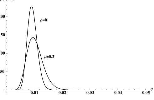
In order to illustrate these calculations we need data which have defaults separately by year. Thus, there is no longer a single integer sufficient statistic—although a vector of integers is not substantially more complicated. To fix ideas, we use a hypothetical bucket of midportfolio corporate bonds of S&P-rated firms in the KMV North American NonFinancial Dataset. Default rates were computed for cohorts of firms starting in September 1993, and running through September 2004. In to-tal there are 2197 asset/years of data and 20 defaults, for an overall empirical rate of 0.00913. The posterior expectation is
Eθ=0.0104 and the posterior standard deviationσθ=0.0029. The corresponding statistics for the binomial model without heterogeneity areEθ=0.0094 andσθ=0.0018. Figure8gives the posterior densities for θ with and without heterogeneity. Allowing for heterogeneity clearly decreases the data informa-tion and, therefore, increases the posterior uncertainty about the long-run default probabilityθ.
Our specification with the correlation at the value specified in the international guidance shows that the data are consider-ably less informative about the default probability in the gener-alized model, even though no new parameters are introduced— i.e., the reduction in data information is not simply a degrees of freedom effect. We next consider the model withρunknown but with a distribution centered on the B2 value. This will give an indication of the sensitivity of the results to the regulatory specification, and will indicate to some extent the data impli-cations forρ.We consider two priors forρ,a beta distribution with standard deviation 0.05 and a beta with standard devia-tion 0.32. These, together with the result forρfixed at its mean value provide coverage of a range of precisions all centered on the B2 value (0.20). In both cases we specify this prior inde-pendently of the prior on the default probability. Of course, this does not imply that the posterior has these quantities indepen-dent and indeed we find positive posterior correlation. The two beta distributions have parameters (12.6, 50.4) and (0.12, 0.48), respectively.
Kiefer: Default Estimation and Expert Information 327
For the intermediate specification with the standard deviation of ρ equal to 0.05, the posterior moments are Eθ=0.0103,
Eρ=0.187, σθ=0.0028, σp=0.0455,andρθρ (the posterior correlation between the default probability and the asset value correlation)=0.119. Thus allowing uncertainty about the value of the asset correlation does not substantially change the result for the parameter of interest,θ.
For the less informative specification with the standard devia-tion ofρequal to 0.32, the posterior moments areEθ=0.0098,
Eρ=0.120, σθ=0.0025, σp=0.0804,andρθρ=0.213. Here too, with very weak prior information about the asset corre-lation, the inference on the interest parameterθ is essentially unchanged. The posterior expectation ofρ is reduced, though there is not much posterior information about this parameter, as might be expected with a fairly rich model and a dataset with few defaults. Note that the posterior expectation is within one standard deviation of the posterior expectation from the inter-mediate model, and in fact is within one standard deviation of the value prescribed by B2.
We estimated this model using direct numerical integration (with Mathematica™ 6.0). Estimation of much more compli-cated models is now in principle straightforward using Markov chain Monte Carlo (MCMC) and related procedures (seeRobert and Casella 2004 andGeweke 2005). These techniques may be useful in the context of validation (essentially specification analysis) procedures that banks are expected to employ. See
OCC(2006).
9. CONCLUSION
I considered inference about the default probability for a midrange portfolio segment on the basis of data information and expert judgement. Examples focus on the sample size of 500; results are also presented for the 1000 observations, some portfolios in this risk range are much larger. These analy-ses are relevant to hypothetical portfolios of middle-risk com-mercial loans. These are predominantly to unrated companies; if rated these would be approximately S&P Baa or Moody’s BBB. I also represented the judgement of an expert in the form of a probability distribution, for combination with the likelihood function. The expert is a practitioner experienced in risk management in well-run banks. The 4-parameter beta distribution seems to reflect expert opinion fairly well. Errors, which would be corrected through additional feedback and re-specification in practice, are likely to introduce more certainty into the distribution rather than less. We consider the possi-ble likely realizations of the sufficient statistic for the speci-fied statistical model. In the default case, the number of re-alizations is linear in the sample size (while the number of potential distinct samples is exponential). Using the expert in-formation, it is possible to isolate the most likely realizations. In the sample of 500, five defaults are expected. In this case, our analysis of zero through nine defaults covers 92% of ex-pected datasets. Our analyses of samples of 1000 covered 97% of the likely realizations. The binomial model is not the only possible model. The one-factor model underlying the B2 cap-ital calculations allows temporal variation in default rates, in-ducing correlation among defaults within periods. This highly
structural model leads naturally to a generalization of the bi-nomial model. The Bayesian analysis remains straightforward and appropriate. An application to a bucket of midportfolio cor-porate bonds is used to illustrate the effects of generalizing the binomial model to allow heterogeneity and correlated de-faults.
At the validation stage, modelers can be expected to have to justify the likelihood specification and the representation of ex-pert information. Analysis of the sensitivity of the results to the prior should be a part of this validation procedure. We propose using a mixture of the expert’s prior and an alternative, less in-formative prior. In our case, we mix the prior with a uniform distribution on the unit interval. While it is not likely that the uniform describes any expert’s opinion on the default proba-bility, mixing in the uniform allows unexpected disagreement between the prior and the data to appear vividly. An example shows that even a trivially small weight on the alternative will do. Of course, within the context of the model, the decision based on the expert’s posterior is correct. A broader view might suggest something wrong with the specification—either of the likelihood or the prior. Perhaps these do not refer to the same risk class, or perhaps the default definitions are inconsistent. The situation is not unlike that arising in ordinary validation exercises in which the model is evaluated in terms of resid-ual analysis or out-of-sample fits. These involve considerations which are relevant but which are outside the formal model. As a result there are a number of different methods in use, corre-sponding to different ways in which models can fail, and expert judgement remains crucial in this less formal context as well as in the formal specification of the likelihood and the prior. For further discussion, seeOCC(2006). Finally, the use of the posterior distribution solely to obtain estimators to insert into the B2 capital formulas is somewhat crude. Risk managers at the bank level might use the full posterior distributions in risk management decisions, calculating, for example, implied distri-butions of losses and probabilities of different levels of losses taking into account not only uncertainty about defaults, but un-certainty about default probabilities. Supervisors and risk man-agement officials might consider the distribution of minimum required capital and choose standards accordingly using a loss function. These possibilities seem not yet to be at hand. The use of a loss function in determining capital is suggested inKiefer and Larson(2004).
ACKNOWLEDGMENTS
Funded by the Danish National Research Foundation. The author thanks Jeffrey Brown, Mike Carhill, Hwansik Choi, Erik Larson, Mark Levonian, Mitch Stengel, and seminar par-ticipants at Cornell University and the OCC. These thanks come with gratitude, but without any implication of agree-ment with my views. Disclaimer: The stateagree-ments made and views expressed herein are solely those of the author, and do not necessarily represent official policies, statements or views of the Office of the Comptroller of the Currency or its staff.
[Received September 2007. Revised September 2008.]
REFERENCES
Basel Committee on Banking Supervision (2004), “International Convergence of Capital Measurement and Capital Standards: A Revised Framework,” Bank for International Settlements. [320,324]
(2005), “Basel Committee Newsletter No. 6: Validation of Low-Default Portfolios in the Basel II Framework,” discussion paper, Bank for International Settlements. [324]
(2006), “International Convergence of Capital Measurement and Cap-ital Standards: A Revised Framework, Comprehensive Version,” Bank for International Settlements. [326]
BBA, LIBA, and ISDA (2005), “Low Default Portfolios,” discussion paper, British Banking Association, London Investment Banking Association and International Swaps and Derivatives Association, Joint Industry Working Group. [324]
Berger, J. O. (1980),Statistical Decision Theory: Foundations, Concepts and Methods, New York: Springer-Verlag. [320]
Berger, J., and Berliner, L. M. (1986), “Robust Bayes and Empirical Bayes Analysis With Contaminated Priors,”The Annals of Statistics, 14 (2), 461– 486. [324]
Chaloner, K. M., and Duncan, G. T. (1983), “Assessment of a Beta Prior Dis-tribution: PM Elicitation,”The Statistician, 32, 174–180. [322]
Cover, T. M., and Thomas, J. A. (1991),Elements of Information Theory, Wiley. [321]
De Finetti, B. (1974),Theory of Probability, Vol. 1, New York: Wiley. [320,322] Diaconis, P., and Ylvisaker, D. (1985), “Quantifying Prior Opinion,” in Bayesian Statistics 2, eds. J. M. Bernardo, M. H. DeGroot, D. Lindley, and A. Smith, Amsterdam: North-Holland, pp. 133–156. [322]
Garthwaite, P. H., Kadane, J. B., and O’Hagan, A. (2005), “Statistical Methods for Eliciting Probability Distributions,”Journal of the American Statistical Association, 100, 780–700. [322]
Gavasakar, U. (1988), “A Comparison of Two Elicitation Methods for a Prior Distribution for a Binomial Parameter,”Management Science, 34 (6), 784– 790. [322]
Geweke, J. (2005),Contemporary Bayesian Exonometrics and Statistics, New York: Wiley. [327]
Gordy, M. B. (2003), “A Risk-Factor Model Foundation for Ratings-Based Bank Capital Rules,”Journal of Financial Intermediation, 12, 199–232. [326]
Halpern, J. Y. (2003),Reasoning About Uncertainty, Cambridge: MIT Press. [320]
Heath, D., and Sudderth, W. (1978), “On Finitely Additive Priors, Coherence, and Extended Admissibility,”The Annals of Statistics, 6, 335–345. [320] Hoogerheide, L. F., Kaashoek, J. F., and van Dijk, H. K. (2007), “On the Shape
of Posterior Densities and Credible Sets in Instrumental Variable Regres-sion Models With Reduced Rank: An Application of Flexible Sampling Methods Using Neural Networks,”Journal of Econometrics, 139, 154–180. [322]
Kadane, J. B., and Wolfson, L. J. (1998), “Experiences in Elicitation,”The Sta-tistician, 47 (1), 3–19. [322]
Kadane, J. B., Dickey, J. M., Winkler, R. L., Smith, W. S., and Peters, S. C. (1980), “Interactive Elicitation of Opinion for a Normal Linear Model,” Journal of the American Statistical Association, 75 (372), 845–854. [322] Kahneman, D., and Tversky, A. (1974), “Judgement Under Uncertainty:
Heuristics and Biases,”Science, 185, 1124–1131. [320]
Kiefer, N. M. (2008), “Default Estimation for Low Default Portfolios,”Journal of Empirical Finance, 16, 164–173. [324]
Kiefer, N. M., and Larson, C. E. (2004), “Evaluating Design Choices in Eco-nomic Capital Modeling: A Loss Function Approach,” inEconomic Cap-ital: A Practitioner Guide, ed. A. Dev, London: Risk Books, Chapter 15. [327]
Lindley, D. V. (1982a), “The Improvement of Probability Judgements,”Journal of the Royal Statistical Society, Ser. A, 145 (1), 117–126. [323]
(1982b), “Scoring Rules and the Inevitability of Probability,” Interna-tional Statistical Review/Revue InternaInterna-tionale de Statistique, 50 (1), 1–11. [320]
Nickell, P., Perraudin, W., and Varotto, S. (2000), “Stability of Rating Transi-tions,”Journal of Banking and Finance, 24, 203–227. [320,326]
Nyarko, Y., and Schotter, A. (2002), “An Experimental Study of Belief Learning Using Elicited Beliefs,”Econometrica, 70 (3), 971–1005. [322]
OCC (2006), “Validation of Credit Rating and Scoring Models: A Workshop for Managers and Practitioners,” Office of the Comptroller of the Currency. [325,327]
Pluto, K., and Tasche, D. (2005), “Thinking Positively,”Risk, August, 72–78. [324]
Ritov, Y. (1985), “Robust Bayes Decision Procedures: Gross Error in the Data Distribution,”The Annals of Statistics, 13 (2), 626–637. [325]
Robert, C., and Casella, G. (2004),Monte Carlo Statistical Methods(2nd ed.), New York: Springer-Verlag. [327]
Savage, L. J. (1954),Foundations of Statistics, New York: Wiley. [320] van der Vaart, A. W. (1998),Asymptotic Statistics, Cambridge: Cambridge
Uni-versity Press. [324]