Full Terms & Conditions of access and use can be found at
http://www.tandfonline.com/action/journalInformation?journalCode=ubes20
Download by: [Universitas Maritim Raja Ali Haji] Date: 12 January 2016, At: 00:20
Journal of Business & Economic Statistics
ISSN: 0735-0015 (Print) 1537-2707 (Online) Journal homepage: http://www.tandfonline.com/loi/ubes20
Another Look at the Identification of Dynamic
Discrete Decision Processes: An Application to
Retirement Behavior
Victor Aguirregabiria
To cite this article: Victor Aguirregabiria (2010) Another Look at the Identification of Dynamic
Discrete Decision Processes: An Application to Retirement Behavior, Journal of Business & Economic Statistics, 28:2, 201-218, DOI: 10.1198/jbes.2009.07072
To link to this article: http://dx.doi.org/10.1198/jbes.2009.07072
Published online: 01 Jan 2012.
Submit your article to this journal
Article views: 166
Another Look at the Identification of Dynamic
Discrete Decision Processes: An Application
to Retirement Behavior
Victor AGUIRREGABIRIA
Department of Economics, University of Toronto, Toronto, Ontario M5S 3G7, Canada (victor.aguirregabiria@utoronto.ca)
This article deals with the estimation of behavioral and welfare effects of counterfactual policy interven-tions using dynamic structural models where all the primitive funcinterven-tions are nonparametrically specified (i.e., preferences, technology, transition rules, and distribution of unobserved variables). It proves the nonparametric identification of agents’ decision rules, before and after the policy intervention, and of the change in agents’ welfare. Based on these results, I propose a nonparametric procedure to estimate the be-havioral and welfare effects of a class of counterfactual policy interventions. The nonparametric estimator can be used to construct a test of the validity of a parametric specification. I illustrate this method using a simple model of labor force retirement, panel data with information on public pension wealth, and a hypothetical reform that delays by three years the eligibility ages of the public pension system in Sweden.
KEY WORDS: Counterfactual policy interventions; Dynamic discrete decision processes; Nonparamet-ric identification; Retirement behavior.
1. INTRODUCTION
Dynamic discrete choice structural models assume that agents are forward looking and maximize expected intertempo-ral payoffs. The structuintertempo-ral functions to estimate in these mod-els represent agents’ preferences and beliefs about uncertain events. These functions are estimated under the principle of re-vealed preference and using microdata on individuals’ choices and outcomes. Dynamic discrete choice structural models have proven useful tools for the assessment of public policy interven-tions, hypothetical or factual, such as unemployment insurance, social security pensions, patent regulation, educational policies, programs on child poverty, and scrapping subsidies, among many others. A common feature of the econometric models in these applications is the parametric specification of the struc-tural functions. These parametric models contrast with the em-phasis on robustness and nonparametric specification in the lit-erature on evaluation of treatment effects (see Heckman and Robb 1985; Manski1990, and, more recently, Heckman and Smith1998and Heckman and Vytlacil 1999, 2005). Though robustness is an important argument in favor of the treatment effects approach, that methodology cannot be used to evalu-ate counterfactual policies and it has limitations in measuring welfare effects and in allowing for transitional dynamics and general equilibrium effects. It is in this kind of problem where dynamic structural models can be particularly useful. The main purpose of this article is to determine conditions under which nonparametrically specified dynamic structural models can be used to estimate the effects of counterfactual policy interven-tions.
Rust (1994) and Magnac and Thesmar (2002) have obtained negative results on the identification of dynamic discrete struc-tural models. These studies show that the principle of revealed preference can identify a value function that combines both preferences and beliefs, but it cannot identify preferences sepa-rately from beliefs, even when the researcher “knows” the time
discount factor and agents’ beliefs. Based on this negative re-sult, this article takes a different look at the problem of non-parametric identification of dynamic decision models. Instead of looking at the separate identification of preferences and be-liefs, I study the identification of the behavioral and welfare effects of counterfactual policy changes. I prove the identifica-tion of agents’ optimal decision rules and value funcidentifica-tions as-sociated with a class of hypothetical policy interventions. This approach is in the spirit of Marschak (1953) who was one of the first econometricians to argue that models that are not fully identified may contain subsets of parameters that are identified and can be used for policy analysis (see also Heckman2000for a discussion of Jacob Marschak’s approach to structural econo-metrics and identification).
In the Rust–Magnac–Thesmar framework, the econometri-cian observes agents’ decisions and some state variables for a random sample of agents. In this article, I assume that the econometrician also observes an outcome variable. This out-come variable is neither a decision nor a state variable, but it is a component of the utility function. Observing this outcome variable is key for the nonparametric identification of the distri-bution of the unobservables. However, this additional informa-tion does not solve the Rust–Magnac–Thesmar underidentifica-tion problem. In particular, the component of the utility funcunderidentifica-tion that is not the outcome variable cannot be identified separately from agents’ beliefs.
A first contribution of this article is to show that, for a wide class of models and counterfactual policies, agents’ be-haviors before and after the policy intervention, and the change in agents’ welfare, are nonparametrically identified. Three as-sumptions are key for this identification result. First, (a) the
© 2010American Statistical Association Journal of Business & Economic Statistics April 2010, Vol. 28, No. 2 DOI:10.1198/jbes.2009.07072
201
outcome variable enters additively in the utility function, and the unobservables affecting this variable are (conditionally) in-dependent of the other unobservables in the utility function. Second, (b) the transition probability function and the discount factor are not affected by the policy. And third, (c) the econo-metrician knows the difference between the utility functions before and after the policy change but does not know either of these two utility functions. I show that, under condition (a), a recursive application of a theorem put forward by Matzkin (1992, 1994) implies the identification of the distribution of the unobservables and of two value functions: the present value of behaving optimally minus the present value of some arbitrary behavior, and the present value of a one-period deviation from the arbitrary behavior. However, knowledge of these value func-tions is not sufficient to identify the one-period utility function or to identify the effects of a general class of counterfactual changes in the structural functions. Instead of imposing ad-ditional restrictions to identify the utility function, the article shows that knowledge of these value functions is sufficient to identify the effects of a relevant class of counterfactual policies. Conditions (b) and (c) characterize the class of counterfactual policies whose effects can be identified without further assump-tions on the primitives of the model.
A second contribution of the article is that it proposes a non-parametric method to estimate the behavioral and welfare ef-fects of counterfactual policy interventions. When the effect of interest is conditional on agents’ state variables, the estimator is subject to the standard “curse of dimensionality” in nonpara-metric estimation: that is, its rate of convergence is not
root-n, and it declines with the number of continuous explanatory variables. However, the estimator of the unconditional average effect is root-nconsistent. Therefore, it is possible to obtain pre-cise estimates of policy effects even when the specification of the structural model contains a relatively large number of state variables. As a third contribution, I apply this method to evalu-ate hypothetical reforms in the rules of a public pension system using data of male blue-collar workers in Sweden. This applica-tion illustrates how the method can be used to obtain meaning-ful estimates of behavioral and welfare effects that do not rely on parametric assumptions on the primitives of the model.
A recent study by Heckman and Navarro (2007) deals with the identification of dynamic discrete structural models. Heck-man and Navarro consider the identification of primitive struc-tural functions; for example, the utility function and the tran-sition probability function of state variables. Their sampling framework is very similar to the one in this article: the re-searcher observes agents’ actions, some state variables, and an outcome variable. As mentioned above, observing an outcome variable does not solve the Rust–Magnac–Thesmar underiden-tification problem. In order to get around this underidentifi-cation, Heckman and Navarro incorporate several restrictions. The most substantial restriction, and the one that clearly dis-tinguishes the Heckman and Navarro model from the approach in this article, is that they assume that the continuation value associated with one of the choice alternatives is known to the researcher; for example, it is “normalized” to zero. This re-striction is also considered in Taber (2000). Though this restric-tion may be needed for the identificarestric-tion of the utility funcrestric-tion, I show in this article that it is not needed for the identification
of the effects of a wide and relevant class of counterfactual ex-periments. Furthermore, if this restriction does not hold in the “true” model, then the predicted effects of some counterfactual policies based on the estimated model can be inconsistent. Ba-jari and Hong (2006) study the identification of a semiparamet-ric dynamic discrete choice game where the probability distrib-ution of the unobservables is parametric (extreme value type 1). Like Heckman and Navarro, they consider the identification of primitive structural functions. They present exclusion restric-tions that can identify players’ utility funcrestric-tions.
The rest of the article is organized as follows. In Section2, I set up the model and the basic assumptions. Section3presents the identification results. Section 4 describes the estimation procedure. The empirical application is featured in Section5. I summarize and conclude in Section6. Proofs of propositions are in theAppendix.
2. MODEL
2.1 Framework and Basic Assumptions
Time is discrete and indexed byt. Agents have preferences defined over a sequence of states of the world between periods 0 andT, where the time horizonTcan be finite or infinite. A state of the world has two components: a vector of state variablesst
that is predetermined before period t; and a discrete decision
at∈A= {0,1, . . . ,J}that the agent chooses at periodt. The set
of feasible choices at timetmay depend on the state:at∈A(st),
withA(st)⊆A. The decision at periodtaffects the evolution of
future values of the state variables. An agent’s preferences over possible sequences of states of the world can be represented by the time-separable utility functionTj=0βjUt(at+j,st+j), where
β∈ [0,1)is the discount factor andUt(at,st)is the current
util-ity function at periodt. Agents have uncertainty about future values of state variables. Their beliefs about future states can be represented by a sequence of Markov transition probability functionsFt(st+1|at,st). These beliefs arerationalin the sense
that they are the true transition probabilities of the state vari-ables. In every periodt, the agent observes the vector of state variablesst and chooses an actionat∈A(st)to maximize the
function at periodt, respectively. By Bellman’s principle of op-timality, the sequence of value functions can be obtained using the recursive expression:
The researcher observes a random sample of agents who be-have according to this model. Agents in the sample are indexed byi∈ {1,2, . . . ,n}. As is typically the case in micro panels, we observe each individual over a short period of time. I consider that each individual is observed for two periods. It is important
to note that in this article the time indext does not represent calendar time but the agent-specific period in the agent’s deci-sion problem. To emphasize this agent-specific time, I refer to
tas theagent’s age. In some parts of the article I will also em-phasize this point by using the variabletito represent agenti’s
age. For each agent in the sample, the econometrician observes his action,ait, and a subvectorxitof the vector of state variables sit, that is,xit⊂sit, and anoutcome variable yitthat contains
in-formation about utility but is not one of the model’s actions or state variables. For instance, in a model of firm behavior the re-searcher may observe firms’ output or revenue, or in a model of individual behavior the econometrician may observe individual earnings. This outcome variable depends on current values of the action and the state variables. I specify this relationship as
yit=Yt(ait,sit), whereYt(·)is theoutcome function; for
exam-ple, a production function. In summary, the researcher’s dataset is
Data= {ait,xit,yit:i=1,2, . . . ,N;t=ti,ti+1}. (3)
The vector of state variablessitcan be decomposed into three
subvectors:sit =(xit, ωit,εit) whereωit represents
unobserv-ables that enter into the outcome function, andεit represents
unobservables that enter into the utility function but not into the outcome function. Bothωitandεitarestructural state variables
in the sense that they have an economic interpretation within the model; for example, a productivity shock, or a temporary shock in health status.
Assumptions1–6 establish the key restrictions that will be used to obtain our identification results. Assumptions1–5refer to the structural functions of the model: preferences, beliefs, and choice set. Assumption6(in Section2.2) defines the class of policy interventions that I consider in this article.
By the law of conditional probability, the transition proba-bility of the state variables,F(si,t+1|ait,sit), can be written as
the product of two transitions, one for the unobservables(ε, ω) and the other for the observablesx: that is, F(si,t+1|ait,sit)=
Pr(εi,t+1, ωi,t+1|xi,t+1,ait,sit)Pr(xi,t+1|ait,sit). Assumption1
establishes conditional independence restrictions on these tran-sition probabilities.
Assumption 1 (Conditional independence). (A) The unob-served state variables have exogenous transition probabilities in the sense that they do not depend on the agent’s current action: Pr(εi,t+1, ωi,t+1|xi,t+1,ait,sit) = Pr(εi,t+1, ωi,t+1|xi,t+1, ωit,
εit); (B) conditional on the contemporaneous value of x,
the variables ε and ω have independent transitions, and ε is not serially correlated: Pr(εi,t+1, ωi,t+1|xi,t+1, ωit,εit) =
Fε(εi,t+1|xi,t+1)Fω(ωi,t+1|xi,t+1, ωit); and (C) the evolution of xit may be endogenous (i.e., dependent on the agent’s actions),
but conditional onxitandait, the vectorxi,t+1does not depend
on ωit and εit, Pr(xi,t+1|ait,xit, ωit,εit)=Fx(xi,t+1|ait,xit).
Under these conditions, the cumulative transition probability of the state variables factors as
F(si,t+1|ait,sit)=Fε(εi,t+1|xi,t+1)Fω(ωi,t+1|xi,t+1, ωit)
×Fx(xi,t+1|ait,xit). (4)
This assumption is similar to Rust’s conditional indepen-dence assumption (see Rust1994). It is weaker than Rust’s be-cause it allows the unobservableωit to be serially correlated.
Relative to the conditional independence assumptions in Heck-man and Navarro (2007), Assumption 1 is neither more gen-eral nor more restrictive. Heckman and Navarro also assume thatεandωare conditionally independent, but they allow for time-invariant unobserved heterogeneity in these unobservables (see their page 365). However, they assume that all the observed state variables (other than the indicator of the lagged stopping decision) follow strictly exogenous stochastic processes that do not depend on the agent’s actions [see their theorem 4, condi-tion (ii)].
Assumption 2(Additivity of the outcome in the utility func-tion). The utility functionUt is additive in the outcome
func-tion. For any possible actiona∈A,
Ut(a,sit)=Yt(a,xit, ωit)+Ct(a,xit,εit), (5)
whereCt(·)is a real-valued function.
Together with the conditional independence in Assump-tion 1, this assumption implies that the utility of alterna-tive a is the sum of two random variables, Yt(a,xit, ωit)and
Ct(a,xit,εit), which are independent conditional on xit. This
assumption is not innocuous and it restricts the structure of the utility function. For instance, in the retirement model of the application in Section5, this assumption implies that an indi-vidual’s utility is the sum of annual earnings and the utility of leisure, and that these two components are independent once we condition on age, marital status, and pension wealth.
For our analysis, it is convenient to decomposeCt(a,xit,εit)
into two additive components: the median ofCt(a,xit,εit)
con-ditional onxit, and the deviation with respect to this median.
For any actiona∈Awe have that
Ct(a,xit,εit)=Mt(a,xit)+ηit(a), (6)
where Mt(a,xit) ≡ Median(Ct(a,xit,εit)|xit) and ηit(a) ≡
Ct(a,xit,εit)−Mt(a,xit). I use η
it to represent the vector {ηit(0), ηit(1), . . . , ηit(J)}. By construction, the random
vari-ables inηithave median zero and are median independent ofxit.
It is possible to show thatηit andεit generate the same
sigma-algebra and that they share some properties. For instance, ifεit
satisfies the conditional independence in Assumption1, thenηit
also satisfies
F(si,t+1|ait,sit)=F
η(ηi,t+1|xi,t+1)Fω(ωi,t+1|xi,t+1, ωit)
×Fx(xi,t+1|ait,xit). (7)
Nevertheless, it is important to note thatεitandηitare different vectors of random variables. Whileεit contains structural
vari-ables with a clear economic interpretation within the model, this is not generally the case forηit. Furthermore, the identifi-cation of the probability distribution ofηit does not imply the identification of the distribution ofεit or of the effect ofεit on
the function Ct(a,xit,εit). However, for the identification
re-sults in this article, we need to know the distribution ofηitand it is not necessary to know the distribution ofεitor the function
Ct(a,xit,εit).
Assumption 3 (Distribution of unobservables). (A) ηit is a
vector of continuous random variables with support the Euclid-ean space; (B) for any value of x, Fη(η|x) is continuously
differentiable in η; (C) ω is a continuous random variable
with support R; and (D) the transition probability function
Fω(ωt+1|xt+1, ωt)is such that for any value of xt+1 and any
strictly increasing function q(·), the conditional expectation
E(q(ωt+1)|xt+1, ωt)=q(ωt+1)Fω(dωt+1|xt+1, ωt) is an
in-creasing function ofωt.
Assumptions 3(A), 3(B), and 3(C) are standard. Assump-tion3(D) establishes that, givenxt+1,ωt+1depends positively
and monotonically on ωt. Though this is clearly a restriction
on the stochastic process of the unobservablesωt, it is also a
common and plausible assumption in many applications.
Assumption 4 (Monotonicity of the outcome function).
(A) The outcome functionYt is strictly monotonic inωit, such
that there is an inverse functionYt−1andωit=Yt−1(ait,xit,yit);
and (B) for any x ∈X and any action a=0, the function
˜
Yt(a,x, ω)≡Yt(a,x, ω)−Yt(0,x, ω)is strictly increasing in
ω, and for any valueu∈Rthere exists a valueω∈Rsuch that
˜
Yt(a,x, ω)=u.
Assumption 4(A) is used to identify point-wise the sample values of the unobserved variable ωit. The monotonicity of
˜
Yt(a,x, ω)with respect toωin Assumption4(B) is used to
iden-tify the distribution functionFη(η|x)from the discrete choices. The strict monotonicity in Assumption4is a strong condition that rules out some interesting cases such as discrete or cen-sored outcome variables. However, it can be relaxed to a cer-tain extent. In particular, Assumption 4 can be replaced by a similar assumption but in terms of an observable variable in the vectorx.
Assumption 4′. There is a continuous observable variable
xK⊆xsuch thatη
itandωitare independent ofxKitand the
func-tionY˜t(a,x, ω)≡Yt(a,x, ω)−Yt(0,x, ω)is strictly increasing
inxK, and for any valueu∈Rthere exists a valuexK∈Rsuch
thatY˜t(a,x, ω)=u.
Under Assumption4′, we do not need to identify point-wise the sample values ofωit. We can exploit the monotonicity of
˜
Yt(a,x, ω)with respect toxK to identify the distribution
func-tionFη(η|x), and we can use a similar approach as in Aakvik, Heckman, and Vytlacil (2005) to identify the distribution ofω without having to identify point-wise the sample values ofωit.
Assumption 5. The set of feasible choice alternatives at time
tdepends only on observed state variables:A(sit)=A(xit).
Assumptions 1 and 5 imply that the optimal decision rule αt(sit) can be described as αt(sit)=arg maxa∈A(x
it){vt(a,xit, ωit)+ηit(a)}, where the functions vt(0,x, ω),vt(1,x, ω), . . . ,
vt(J,x, ω)are choice-specific value functions and they are
de-fined as
vt(a,xt, ωt)≡Yt(a,xt, ωt)+Mt(a,xt)
+
max
a′∈A(xt+1){
vt+1(a′,xt+1, ωt+1)+ηt+1(a′)}
×F(dst+1|a,xt, ωt). (8)
The optimal decision rule represents individuals’ behavior. In-dividuals’ welfare is given by the value function Vt(st)=
maxa∈A(xt){vt(a,xt, ωt)+ηt(a)}. For the econometric analysis,
it is convenient to define versions of these functions that are
integrated over the unobservables inηt. The choice probability function is defined as
Pt(a|xt, ωt)≡
I{α(xt, ωt,η
t)=a}Fη(dηt|xt). (9)
The integrated-valued function is
¯
Vt(xt, ωt)≡
Vt(st)Fη(dη
t|xt) =
max
a∈A(xt)
{vt(a,xt, ωt)+ηt(a)}Fη(dη
t|xt). (10) 2.2 Policy Interventions
Consider a hypothetical policy intervention that modifies the current utility function. LetUtbe the utility function in thedata
generating process, and letU∗t be the utility function under the counterfactual policy. Assumption6describes the class of pol-icy interventions that I consider in this article.
Assumption 6. The counterfactual policy can be represented as a change in the utility function from functionUtto function
Ut∗such that: (A) the econometrician knows the difference be-tween the two utility functions [i.e., the econometrician knows the functionτt(a,s)≡U∗
t(a,s)−Ut(a,s)]; and (B) the function
τt(a,s)does not depend onη, that is,τt(a,s)=τt(a,x, ω).
The functionτt represents the policy intervention and it is
known to the researcher, though the functionsUtandU∗t are
un-known. It may depend on(a,x, ω)in a completely unrestricted
way, but it cannot depend on the unobservableη.
Let{Pt,V¯t}and{P∗t,V¯t∗}be the choice probability functions
and the integrated value functions before and after the policy in-tervention, respectively. I represent the behavioral effects of the policy by comparing the functionsP∗t andPt. Similarly, the
dif-ference between the functionsV¯t∗andV¯trepresents the welfare
effects of the policy.
2.3 An Example: A Model of Capital Replacement
The example is a simplified version of the model in Kasahara (2009), which examines the impact on firms’ equipment invest-ment of a temporary increase in import tariffs in Chile. A firm produces a good using capital (a machine) and perfectly flexi-ble inputs. The firm has multiple plants and each plant consists of only one machine. Production at different plants is indepen-dent and there are constant returns to scale. Therefore, we can concentrate on the decision problem for an individual plant or machine. The current profit of a plant is equal to variable prof-its minus maintenance costs and machine replacement costs. Letxtrepresentthe time since last machine replacement,or the
age of the existing machine at the beginning of montht. And letat∈ {0,1}be the indicator of the decision of replacing the
old machine by a new machine at the beginning of month t. Therefore, the age of the machine that is used during month
tis(1−at)xt. The variable profit during monthtdepends on
the age of the machine and on a productivity shockωt, and it
is represented by the variable profit functionY((1−at)xt, ωt).
The amount of variable inputs is a deterministic function of the age of the machine and the productivity shock and therefore it
is implicit in the functionY(·). The productivity shockωt
fol-lows a Markov process, and the transition rule of the age of the machine isxt+1=(1−at)(xt+1)+at. The profit function has
the following form:
Ut=Y((1−at)xt, ωt)−CM((1−at)xt, εMt )
−atCR(xt, εRt). (11)
CM(·,·)is the maintenance cost, which depends on the age of the machine and on a random shockεtMthat is unobservable to the researcher.CR(·,·)is the replacement cost net of the scrap-ping value of the retired capital. The replacement cost is paid only if the machine is replaced, and it depends on the age of the old machine and on a random shockεtRthat is also unob-servable to the researcher. In this model, Assumption1implies that the cost shocksεtR andεMt are independently distributed over time (though their distribution may depend on the age of the machine) and distributed independently of the productivity shockωt. The specification of the profit function imposes the
additive separability of Assumption2. Using the same decom-position as in expression (6), I can write the profit function as
Ut=Y((1−at)xt, ωt)−Mt(at,xt)−ηt(at), (12)
where Mt(0,xt) ≡ Median(CM(xt, εtM)|xt), Mt(1,xt) ≡
Median(CM(0, εMt ) + CR(xt, εRt)|xt), ηt(0) ≡ CM(xt, εMt ) −
Mt(0,xt), andηt(1)≡CM(0, εtM)+CR(xt, εRt)−Mt(1,xt).
As-sumption1(B) implies thatηt(0)andηt(1)are independent of ωt.
Suppose that we are interested in evaluating the effects of a counterfactual policy that modifies firms’ replacement costs. This policy tries to promote the retirement of old capital by providing a replacement subsidy that depends on the age of the old machine. The amount of the subsidy is
τ (at,xt)=
⎧ ⎪ ⎨ ⎪ ⎩
0 if xt<x∗low
at(λ0−λ1[xt−xlow∗ ]) if xhigh∗ ≤xt≤x∗low
0 if xt>x∗high,
(13)
where{λ0, λ1,x∗low,x∗high}are parameters that characterize the policy, and they have the following properties:λ0>0,λ1>0, and(x∗high−x∗low)≤λ0/λ1. The subsidy is zero if replacement takes place too early (i.e., before agex∗low) or too late (i.e., after agex∗high). For replacement ages within the range[x∗low,x∗high], the subsidy is strictly positive and it decreases linearly with the age of the machine.
3. IDENTIFICATION
Suppose that we have a random sample of individuals with information on the variables{aiti,ai,ti+1,ti,xiti,xi,ti+1,yiti,
yi,ti+1}. As usual, I study identification with a very large (i.e., infinite) sample of individuals. Furthermore, I assume that the sample has variability over the whole support of the observ-able variobserv-ables,A2× [1,T] ×X2×Y2. This assumption of full-support variation is needed to identify the reduced form of the model. For the sake of simplicity, I concentrate on binary choice models:a∈ {0,1}. For notational simplicity I usePt(x, ω)to
denote Pt(1|x, ω). Also, to simplify notation, I use Fηt(·) to
represent the distribution of ηt conditional on xt at period t
(i.e., I omitxtas an argument).
3.1 Preliminaries
I assume that the outcome functionYt(·)is identified
with-out having to estimate the rest of the structural model. There are different conditions under which one can consistently esti-mate wage equations or production functions using instrumen-tal variables or control function approaches that do not require the estimation of the complete structural model (see Olley and Pakes1996and Imbens and Newey2006). The empirical appli-cation of retirement behavior in Section4provides an example for the identification of Yt(·). Following most of the literature
on dynamic discrete structural models, I assume that the dis-count factorβis known to the researcher.
GivenYt(·), Assumption4(A) implies that we can recover the
sample values of unobservables{ωit}asωit=Yt−1(ait,xit,yit).
That is, the sample values ofωitiandωiti+1are identified point-wise, and we can treat these variables as observables. Then, As-sumption1implies that the transition probability functionsFx
andFωare nonparametrically identified. We can identifyFxon
A×X2from the transition frequencies Pr(xi,t
i+1|aiti,xiti)in the data.Fω is also identified onR×R×X from the frequencies
Pr(ωiti+1|ωiti,xiti)in the data. It is also clear that we can iden-tify the choice probability functions Pt(x, ω) onX×R from
the frequencies Pr(aiti =1|xiti, ωiti,ti=t) in the data. How-ever, without further restrictions, we cannot identify the struc-tural functions {Ct,Fεt}or even the semi-structuralfunctions {Mt,Fηt}. Instead, this article considers the identification of the functions P∗t and (V¯t∗− ¯Vt) associated with a counterfactual
policy intervention.
The following Proposition, based on Matzkin (1994), will be used for some of the identification results.
Proposition 1(Based on Matzkin1994). Consider a binary choice model, a=I{η≤W+ϕ(X)}, where a,W, andX are observable variables to the econometrician,ηis unobservable, andϕ(·)is a real-valued function. Consider the following def-initions:SX⊆RK is the support of the vectorX;ϕ0is the true
function ϕ in the population; and Fη0|X is the true CDF of η conditional on X. Assume that: (i)η and W are independent conditional onX; (ii) for anyX∈SX, the CDFFη0|X is strictly
increasing inη, its support isR, andF0η|X(0)=0.5 (zero condi-tional median); (iii) the distribution ofWconditional onXhas a Lebesgue density that is everywhere positive onR; and (iv) for anyX∈SX, there is a value W∈Rsuch thatW+ϕ0(X)=0.
Under these conditions, the functionϕ0is identified onSXand
the functionFη0|X is identified onR.
An implication, or corollary, of Proposition 1 is the fol-lowing. Consider the model and the conditions of Proposi-tion 1. Define the counterfactual choice probability function
P∗(X,W)≡F0η|X(W +ϕ0(X)+π(X,W)), where π(X,W) is a function fromSX×RintoRthat is known to the
econometri-cian. Then,P∗is identified onSX×R, such that
P∗(X,W)=F0η|X(W+ϕ0(X)+π(X,W))
=P0(X,W+π(X,W)). (14) McFadden (1981) defined the social surplus function of a random utility model as the difference between the expected utility of behaving optimally minus the expected utility of an arbitrary (suboptimal) behavior. Proposition2is a corollary of theorem 5.1 in McFadden (1981), and it establishes that the
cial surplus function depends on the optimal choice probability and the CDF of the unobservables only. In the context of a dy-namic discrete choice model, Propositions2and3(below) are key to showing that Matzkin’s proposition 1 can be applied re-cursively to obtain the identification of certain value functions.
Proposition 2. Consider the utility maximization problem max{u(0)+η(0),u(1)+η(1)}, and the following definitions.
Gis the expected utility of behaving optimally minus the ex-pected utility of choosing alternative zero (McFadden’s social surplus), that is,
G≡
max{u(0)+η(0),u(1)+η(1)}dFη(η)−u(0).
Pis the probability that alternative 1 is the optimal choice: that is,
P≡
I{u(0)+η(0) <u(1)+η(1)}dFη(η).
AndFη˜ is the CDF of the random variableη˜≡η(0)−η(1).
IfFη˜is a continuous and strictly increasing function, then the
social surplus G depends on P and Fη˜only. That is, G=
max{0,F−η˜1(P)− ˜η}dFη˜(η)˜ .
Going back to the dynamic binary choice model, Proposi-tion 3 provides a representation of the choice-specific value functionsvt(a,xt, ωt)that will be useful to prove the
identifica-tion results. The proposiidentifica-tion establishes that we can decompose additively the differential value functions vt into three
func-tions. This decomposition is not arbitrary. I show in Section3.2 that we can identify these three components of the value func-tion, and that these components, together with the CDF ofη˜t,
can be used to construct the counterfactual choice probability functionP∗t.
Proposition 3. For any aget, the choice-specific value func-tionvtcan be written as
vt(a,x, ω)=VY
t (a,x, ω)+VtM(a,x)+VtOPT(a,x, ω), (15)
where:VtY(a,x, ω)is the expected, discounted value of the sum
of current and future realizations of the outcome variableyif the current choice isaand then alternative 0 is chosen forever in the future;VtM(a,x)is the expected, discounted value of the
sum of current and future realizations of the componentM of the utility function if the current choice is aand then alterna-tive 0 is chosen forever in the future; andVtOPT(a,x, ω)is the
value of behaving optimally in the future minus the value of al-ways choosing alternative 0, given that the current choice isa. These functions can be obtained recursively as follows: at last periodT,VTY(a,x, ω)=YT(a,x, ω),VM
3.2 Identification of Counterfactual Policy Effects
I present here identification results in the context of a fi-nite horizon model, that is, T <∞. However, the proof can be extended to infinite horizon models. The proof of iden-tification in a model with infinite horizon appears in an earlier version of this article, which is available online at ideas.repec.org. The factual choice probability function is
Pt(x, ω)=Fη˜t(vt(1,x, ω)−vt(0,x, ω)), or, given Proposition3 ω). The value functionVtOPT depends on the agent’s future op-timal behavior and therefore on the opop-timal choice probability functions from periodt+1 until period T. Proposition 4 es-tablishes the identification of the functionsFη˜t,V˜tY,V˜tM, and
˜
VtOPT.
Proposition 4. Suppose that Assumptions1–5hold and that the discount factorβ is known. Then, for any periodt≤T, the functionsFη˜t,V˜tY,V˜tM, andV˜tOPT are identified.
The value V˜tM(x) depends on M˜t(x), the future utilities
{Mt+j(0,xt+j):j>0}, the transition probability function ofx,
and the time discount factorβ. Without further restrictions, the identification of the functions{ ˜VtM}does not provide identifica-tion of the one-period utility funcidentifica-tionMt(a,x), or even of the
differential utility function M˜t(x)≡Mt(1,x)−Mt(0,x). The
one-period utility function is not identified. As in the case of static discrete choice models, there is a “normalization” restric-tion that implies the identificarestric-tion of utility funcrestric-tionMt(a,x).
If we assume thatMt(0,x)=0 for any periodtand any value of x, then, using the definition ofV˜M
t in Equation (16), it is simple
to verify thatVtM(0,x)=0 andV˜M
t (x)=VtM(1,x)=Mt(1,x).
However, this “normalization” is not innocuous. If the normal-ization restriction is not true (and we expect that to be the case in most applications), the estimated model will imply incon-sistent predictions of the effects of certain policy interventions, such as those that modify transition probabilities of the state variables or the time discount factor.
Next, we show that, despite the fact that we cannot identify individuals’ utility functions, we can identify the behavioral and welfare effects of counterfactual experiments in the class defined in Assumption 6. Define the counterfactual outcome functionYt∗(a,x, ω)≡Yt(a,x, ω)+τt(a,x, ω), whereτt(·)is
the function defined in Assumption6. Therefore, the counter-factual choice probability function is
whereV˜tY∗, V˜tM∗, and V˜tOPT∗ are the counterfactual versions of V˜tY, V˜tM, and V˜tOPT, respectively. It is clear that VtY∗ is known, and thatVtM∗=VtM. Therefore, by Proposition4, the functionsV˜tY∗ andV˜tM∗ are identified. Also, note that all the primitives that enter into the value functionV˜tOPT∗ (i.e., tran-sition probabilities, distribution ofη˜, and discount factor) are policy invariant: they are the same before and after the policy change. Therefore, the only way in which the value function
˜
VtOPT∗ is affected by the policy change is through the change in the optimal behavior between periodst+1 and T, that is, through the change in the optimal choice probabilities between
t+1 andT. To emphasize this aspect, I represent the functions
VtOPT(a,x, ω)andVOPT∗
t (a,x, ω)asV˜tOPT(x, ω; {Pt+j:j>0})
andV˜tOPT(x, ω; {P∗
t+j:j>0}), respectively. Taking into account
these considerations, we can write the counterfactual choice probability functions as follows:
Proposition5establishes the identification of the counterfactual choice probabilities.
Proposition 5. Suppose that Assumptions 1–6 hold and that the discount factor β is known. Then, the counterfactual choice probability functions {P∗t}are identified overSX×R.
These probability functions can be obtained using the follow-ing method. Startfollow-ing at the last period,t=T, the probability
P∗t(x, ω)can be obtained recursively as
P∗t(x, ω)=Pt(x, ω∗
t(x, ω)), (20)
whereω∗t(x, ω)is a function fromSX×RintoRthat is
implic-itly defined as the valueω∗t ∈Rthat solves the equation
˜
VtY(x, ω∗
t)+ ˜VtOPT(x, ωt∗; {Pt+j:j>0}) = ˜VtY∗(x, ω)+ ˜VOPT
t (x, ω; {P∗t+j:j>0}). (21)
Proposition6establishes the identification of the welfare ef-fect functionV¯t∗− ¯Vt.
Proposition 6. Under the conditions in Proposition 5, the welfare effect functionV¯t∗− ¯Vtis identified. We can obtain this
function as: for a random sample ofN individuals. For any u∈R, define
wut(x) as the value of ω that solves the equation V˜Y
mation method proceeds in two steps.
Step 1. Estimation of the outcome functionY, transition den-sity functionsfω andfx, factual choice probability functionPt,
and threshold functionw0t.
First, we estimate the outcome function. Given this estimated function, we can get the residuals ωˆiti = ˆY
−1
ti (yiti,aiti,xiti) at every observation i. For the derivation of asymptotic proper-ties, I assume that the outcome function is either parametrically or semiparametrically specified such that the residuals{ ˆωiti}are root-nconsistent estimates of the trueω’s. This implies that the rate of convergence of{ ˆωiti}to{ωiti}is faster than the conver-gence of the kernel estimators that I define below. Therefore, we can ignore the estimation error in{ ˆωiti}in the derivation of the asymptotic properties of the estimator of policy effects.
Given { ˆωiti}we can construct procedures to estimate non-parametrically transition densities fω(ω′|ω) and fx(x′|a,x),
choice probabilityPt(x, ω), and threshold valuesw0
t(x)for
ar-bitrary values of(t,x,x′, ω, ω′,a). These procedures are called
by the estimators in Step 2. For instance, we can use a ker-nel method to estimate the transition densities fω(ω′|ω) and
fx(x′|a,x). Similarly, a kernel estimator of the choice
probabil-ily obtained using Newton’s method. That is, starting at some initialω0, we obtain a sequence of values{ωk:k≥0}using the
recursive formulaωk+1=ωk− ˆPt(x, ωk)/(∂Pˆt(x, ωk)/∂ω). We
iterate in this formula until|ωk+1−ωk|is smaller than a pre-specified small constant. SincePˆt(x, ω)is strictly increasing in
ω, Newton’s method always converges to the unique solution of the equation. In some applications, the kernel estimate of the functionP may not be strictly monotonic inω. Monotonicity ofPˆis necessary for the subsequent estimation of the effects of the counterfactual policy. We can impose monotonicity using the isotonic smooth (IS) kernel estimator proposed by Muker-jee (1988) and Mammen (1991).
Step 2. Recursive (backward induction) estimation of the functions{P∗t},{ ˜VtM}, and{Fη˜t}.
function ofx. Then there is a closed form expression for the
estimator ofω∗T(x, ω):
(b) Based on Proposition5, a consistent estimator ofP∗T(x, (e) By Proposition 4, for u∈R a consistent estimator of
Fη˜T(u)isPˆT(x,wˆu
If(x, ω)includes several continuous state variables, the
multi-ple integral may be approximated using Monte Carlo integra-tion in order to reduce computaintegra-tion time. Similarly, we can ob-tain a consistent estimator ofV˜TOPT−1∗(x, ω). there is not a closed-form analytical expression for the solution to this equation. However, given thatVˆTY−1(x, ω)+ ˆVOPT
T−1(x, ω) is strictly increasing inω, the solution to this equation can be easily obtained using Newton’s method. Again, the unique solution to this equation can be obtained us-ing Newton’s method.
Remark 1. The computational cost of estimating the se-quence of choice probability functions{P∗t}is equivalent to the cost of solving the dynamic programming problem once.
Remark 2. Under standard regularity conditions, our kernel estimator of{P∗t}is consistent and asymptotically normal, and its rate of convergence is
NbkN, where bN is the bandwidth
andk is the number of continuous variables in the vector of state variables(x, ω). The speed of convergence declines with
the number of continuous regressors. In applications with more than two or three continuous state variables, the estimator of the functionP∗t can be quite imprecise unless the number of observations in our dataset is very large. However, there are situations in which we may be interested inpartial meansof the policy effects. A partial mean of the policy effect is an average of P∗t(xt
i, ωti)−Pt(xti, ωti)over some state variables holding other state variables constant. In the literature on evaluation of treatment effects, these partial means are called (conditional) average treatment effects (ATE). Letzibe a vector included in (xt
i, ωti), and letx(−z)irepresent the vector(xti, ωti)excluding
zi, such that(xt
i, ωti)=(zi,x(−z)i). Then, the ATE conditional onzitaking a constant valuezis:
ATE(z)=EP∗t
Whenzi does not include any variable, we have the
uncondi-tional ATE, that is,ATE=E(P∗t
i(xti, ωti)−Pti(xti, ωti)). A con-sistent estimator of the (conditional or unconditional)ATE is simply the sample mean of the kernel estimatorPˆ∗ti(z,x(−z)i)−
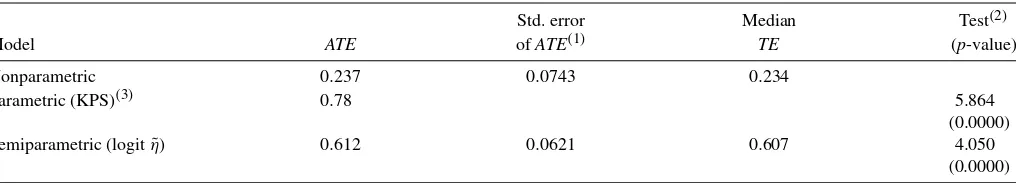
Newey (1994) studies the asymptotic properties of a partial mean of kernel estimates. He shows that averaging out some continuous conditional variables implies an improvement in the rate of convergence of the estimator. Furthermore, averaging over all the (continuous) state variables to obtain the uncon-ditional ATE provides an estimator that is root-n consistent. Therefore, the nonparametric approach in this article may pro-vide precise and meaningful estimates of average policy effects even when the model has a relatively large number of continu-ous state variables and the dataset does not contain many obser-vations. The empirical application in Section5is an example of this.
Remark 3. Based on the results presented in Remark2, it is possible to use our estimator of ATE, based on our nonpara-metric model, to define the following test of a paranonpara-metric spec-ification. LetATEnp andATEpbe the estimators ofATEusing
our nonparametric model and using a parametric model, respec-tively. Under the null hypothesis that the parametric model is
correctly specified, we have that
ATEnp−ATEp
Var(ATEnp−ATEp)
∼aN(0,1), (30)
where∼ameans “is asymptotically distributed as.” The
asymp-totic variance Var(ATEnp−ATEp)can be approximated using a
bootstrap method (see Remark4below). An interesting feature of the test of specification is that it tests the validity of a para-metric model only in the context of estimating a specific pol-icy effect. That is, some specifications may be invalid for some policy experiments but perfectly valid for other policy experi-ments.
Remark 4. In the empirical application in Section 5, I use a bootstrap method to approximate the standard errors of esti-mated average policy effects (unconditional ATEs). The method is a nonparametric bootstrap that resamples the data and repli-cates the whole estimation procedure for each bootstrap sam-ple. Define a block as an individual’s history of observable choices and state variables in the sample. The sample can be described as N blocks, which are independent random draws from a certain population. The bootstrap sampling method that I use takes random draws (independent and with replacement) of blocks from the sample. I take B=500 bootstrap sam-ples of size N; that is, each bootstrap sample has the same number of blocks/individuals as the original sample. The boot-strap standard error of the estimateATE is just the square root of (B−1)−1Bb=1(ATEb−ATE)2, where ATEb is the
esti-mate of the ATE using thebth bootstrap sample and ATE is
B−1Bb=1ATEb.
5. AN APPLICATION
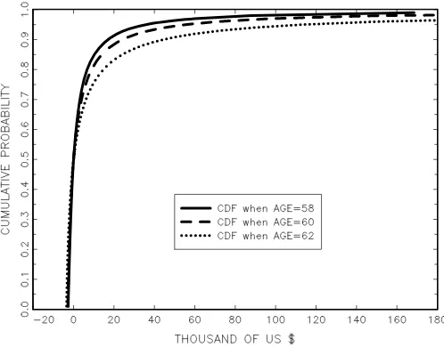
This section presents an application of this methodology to evaluate the effects of a hypothetical reform in the social secu-rity pension system in Sweden. The main purpose of this ap-plication is to illustrate the implementation of the method and to show that it can provide meaningful results. Our model of retirement behavior follows Rust and Phelan (1997) and Karl-strom, Palme, and Svensson (2004). The hypothetical reform consists of a delay of three years in the eligibility ages of the public pension system. The minimum age to claim a public pen-sion increases from 60 to 63 years and thenormalretirement age increases from 65 to 68. This type of reform has been and is still being considered in many Organization for Economic Cooperation and Development (OECD) countries.
Additivity of the outcome variable in the utility function (As-sumption2) and conditional independence between the unob-servables in the outcome function and in the rest of the util-ity function (Assumption1) are key conditions to implement our method. In order to have a model of retirement that satis-fies these assumptions, I impose the following restrictions in the model below: (a) the utility function is additively separa-ble in consumption and leisure; (b) the utility of consumption belongs to the CRRA family and the relative risk aversion pa-rameter is known to the researcher; (c) in every period, con-sumption is equal to disposable income; and (d) conditional on age, marital status, and public pension wealth, there is indepen-dence between the unobservable in labor earnings and the unob-servables in the utility of leisure. These are strong assumptions. In particular, assumption (c) rules out consumption smoothing
and accumulation of private wealth, which is an obvious substi-tute for public pension wealth. Therefore, in our policy analy-sis we assume that when the public pension system becomes less generous (through a delay in eligibility ages), individuals do not decide to reduce their consumption before retirement in order to accumulate wealth and to retire not much later than they planned before the policy change. This type of response is ignored by our model. Interestingly, this assumption is also present in most of the literature on structural models of retire-ment behavior, for example, Berkovec and Stern (1991), Rust and Phelan (1997), Karlstrom, Palme, and Svensson (2004), or, more recently, Bound, Stinebrickner, and Waidmann (2009). Some important exceptions are the recent papers by French (2005), Blau (2008), and van der Klaauw and Wolpin (2008).
5.1 A Model of Retirement Behavior
Every year, individuals decide whether to continue working (at=1) or to retire and claim social security pension benefits
(at=0). This decision is irreversible. Individuals have a utility
function that is additively separable in consumption (Ct) and
leisure (Lt). More specifically, ˜
Ut=UC(Ct)+UL(Lt,t,mt,εt), (31)
wheretrepresents age,mt is marital status, and εt is an
indi-vidual idiosyncratic shock in the utility of leisure that is unob-servable to the econometrician (e.g., unobserved health status). These variables capture individual heterogeneity in the utility of leisure. If the individual works, hours of leisure are equal to L¯1 and annual earnings are equal to labor earnings Wt. If
the individual decides to retire, then hours of leisure are L¯0 and earnings are equal to retirement benefitsBt. Thus, we can
write leisure asLt=atL¯1+(1−at)L¯0and annual earnings as
Yt=atWt+(1−at)Bt. Labor earnings depend on age, marital
status, and a wage shock:
Wt=exp{hW(mt,t)+ωt+1}. (32)
hW(·)is a function andωt+1is a wage shock. This shock fol-lows a Markov process with transition ruleωt+1=ρ(ωt)+ξt+1, where ρ(·) is a function and ξt+1 is the innovation of the process. The individual knowsωt when he decides whether to
retire at aget, but he does not know the innovationξt+1. This assumption is similar to the one in Rust and Phelan (1997), and it is important for the identification of the wage function (see below). Retirement benefits depend on current age (t), retire-ment age (rat), andpension points(ppt):Bt=B(t,mt,rat,ppt).
I describe this function in Section5.2below.
The state variables of the model are εt, ωt, and xt =
(t,mt,rat,ppt). Note that retirement status (i.e., at−1) is im-plicitly given by retirement age. Since the individual has uncer-tainty about current labor earnings, the relevant current utility is the expected utilityUt≡Et(U˜t), where the information set at
periodtis(at,xt, ωt,εt):
Ut≡Et(U˜t)
=Et(UC(Ct))+UL(atL¯1+(1−at)L¯0,t,mt,εt). (33)
In order to have a utility functionUt with the form postulated
in Assumptions1 and2, we need the value of Et(UC(Ct))to
be an observable outcome variableyt for the researcher. If we
could observe individuals’ consumptionCt, we would need
rel-atively weak assumptions to have that structure. However, we do not observe individual consumption. Instead, we observe la-bor earningsWtfor those individuals who are working and
re-tirement benefitsBt(either potential or actual benefits) for every
individual, working or not. I assume that consumption is equal to earnings,Ct =Yt, and that the utility of consumption is a
CRRA function; that is,UC(Ct)=Cαt, whereαis the
parame-ter of relative risk aversion. Furthermore, I also assume that the risk aversion parameter is known to the researcher. Under these conditions, we have that
I conclude this subsection by presenting sufficient conditions for the identification of the outcome function Y(·). Since the pension benefits function B(xt) is known and the risk
aver-sion parameter α is assumed to be known to the econome-trician, we have to identify only the labor earnings function. A least-squares estimation of the log-wage equation log(Wt)=
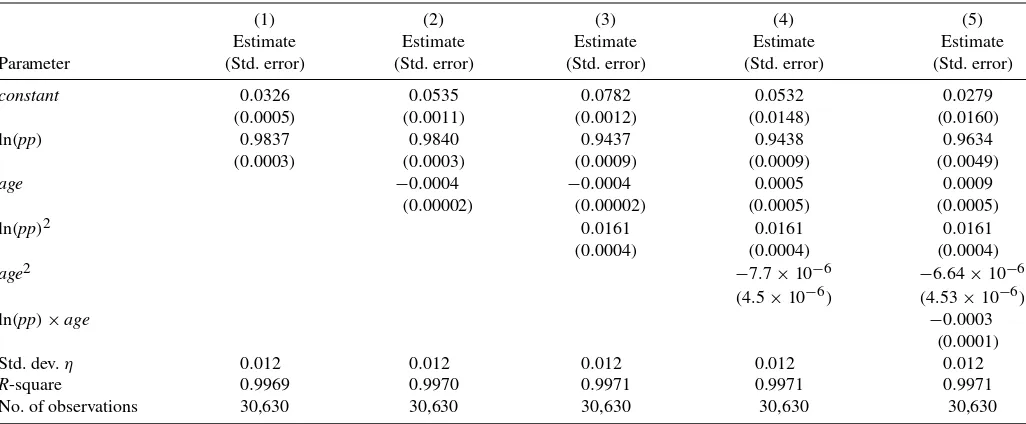
hW(mt,t)+ωt+1(using the sample of observations withat=1)
suffers from selection bias because ωt+1 is not mean inde-pendent of the individual’s choice at period t. However, the Markov structure of the wage shock and our assumption on the arrival of information provide moment conditions that can be used to nonparametrically estimate the functionshW(·)and ρ(·). Consider the subsample of individuals working at pe-riods t and t−1, that is, at=at−1=1. For these individ-The innovationξt+1is iid over time and unknown to the indi-vidual when he makes his working decision at period t, or at periodt−1. This implies thatξt+1is independent of(at,at−1), and it is also independent of xt andWt−1. The orthogonality
conditionsE(ξt+1|at=1,at−1=1,xt,Wt−1)=0 provide
mo-ment conditions that can be used to estimate the functionshW(·)
andρ(·).
5.2 Social Security Pensions and the Counterfactual Reform
I present here a brief description of Sweden’s public pen-sion system during the sample period 1983–1997. For a more detailed explanation, see section 2 in Karlstrom, Palme, and
Svensson (2004, hereafter KPS). I discuss first the pension ben-efits function,B(x), and then the rules for accumulation of
pen-sion points.
In Sweden, the measurement unit for the amount of pension benefits is the so-calledbasic amount(BA). This measure is in-dexed by the consumer price index (CPI), and it was equal to $4,765 U.S. dollars in 2003. Notice that to translate Swedish kronas into U.S. dollars (of the year 2003), I have used an ex-change rate of 8.1 Swedish kronas per U.S. dollar. An individ-ual younger than 60 years old is not entitled to receive public pension benefits. Therefore,B(x)=0 fort<60. Of course,
in-dividuals can retire before age 60, but they cannot claim and receive benefits until they become 60 years old. LetB¯65(m,pp) represent the amount of annual pension benefits that the individ-ual is entitled to if he/she retires at age 65 (see below). Then, for agest≥60, we have that
κ1 is a permanent actuarial reduction in benefits per year of early retirement.κ2is a permanent actuarial increase in benefits per year of delayed retirement. For our sample period, 1983– 1997, the values of these parameters wereκ1=6.0% per year (0.5% per month) and κ2=8.4% per year (0.7% per month). The amount B¯65(m,pp) is the combination of three pension programs: basic pension (BP), special supplementary pension (SSP), and normal supplementary pension (NSP). More specif-ically,
¯
B65(m,pp)=BP(m)+min{SSP,NSP(pp)}. (37) The basic pensionBP(m)depends on marital status but not on the individual’s pension points. It is equal to 96.0% of theBA
(i.e., $4,574 per year) if the individual is single and 78.5% of theBA(i.e., $3,740 per year) if married. TheSSPapplies only if the individual’s normal supplementary pension is not large enough, that is, ifNSP(pp) <SSP. It is the same for every in-dividual and is equal to 55.5% of theBA. The normal supple-mentary pensionNSP(pp)is the most important part of pension benefits for most individuals. It is proportional to the individ-ual’s pension points:NSP(pp)=0.6∗pp∗BA. As I described below, pension points can take values between 0 and 6.5. There-fore, the range of variation of the annual pension benefits upon retirement at age 65 (i.e., the range of variation ofB¯65(x)) is
[1.515∗BA,7.46∗BA](i.e., between $7,219 and $35,547) for a single person, and[1.34∗BA,7.285∗BA](i.e., between $6,385 and $34,713) for a married person. The range of variation of actual pension benefits is larger because individuals retire at different ages, before and after age 65.
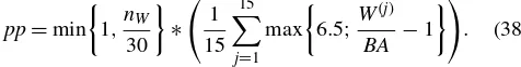
Pension points are a deterministic function of an individual’s whole history of earnings. Every year, an individual with an-nual labor earningsWgreater thanBAobtains an amount of so-cial security points between 0 and 6.5, according to the formula max{6.5;BAW −1}. The pension points are equal to the average social security points over an individual’s best 15 years of earn-ings, adjusted by a factor that depends on the total number of years with earnings greater than theBA. In order to provide an explicit formula, let{W(1),W(2), . . . ,W(15)}be the annual labor