ISSN:2088-5520 C4-64
Spatial Patterns of Poverty in Central-Java Province
Irwan Susanto, Winita Sulandari, Bowo Winarno
Department of Mathematics, Faculty of Mathematics and Natural Sciences Sebelas Maret University
Surakarta, Indonesia email: [email protected]
Abstract
—
Poverty is one of the key issues in development program of Indonesia government. Poverty can be caused by geographical factors, namely the natural conditions, such as climate, density of forest, etc. Therefore, poverty problem tend to be spatially dependent. Spatial dependence is the propensity for nearby locations to influence each other and to possess similar attributes. A measure of the similarity of attributes of locations is called spatial autocorrelation. Spatial autocorrelation measure and analyze the degree of dependency among observations in a geographic spaceThis paper examines spatial patterns of poverty in Central Java Province with spatial autocorrelation using spatial analysis open source software. Through open source software OpenGeoDa, it can be shown that the poverty of certains districts in Central Java Province have significantly spatial autocorrelation and there are some spatial cluster poverty in Central Java which are spatial influenced by density of forest as geographical factor.
Keywords : Spatial pattern, Poverty, Central-Java, Spatial Autocorrelation
I. INTRODUCTION
Poverty is a problem experienced by some countries especially development countries. Factors that affect poverty every country is different, in Indonesia the factors that influence the level of poverty of the population is divided into food commodities (rice, sugar, instant noodles, eggs, tempe and tofu) and non-food commodities (housing, clothing, education and health ) as being analyze in [6]. Efforts of various countries in addressing poverty is certainly not the same, this is adjusted by the condition of a country's well geographical conditions, population or other conditions. Indonesia is a developing country, which until now still has a number of people classified as poor. Number of poor in Indonesia in 2010 amounted to 31.02 million people or about 13,33% and most of the poor live in rural areas which is about 63.47%. Central Java is one of the provinces in Indonesia with a total area of 3.25 million hectares or about 25.04% of the island of Java (1.70% of Indonesia) with a population of 2010 reached 32.38 million people including categories of home poor households. The poverty people in Central Java in 2010 stands at 5.3 million people [7]. In addition the study based National Disaster Management Agency [5], the poverty index of Central Java is above 20, giving an indication that the Central Java is included in the poverty-prone areas.
Currently, it has been many efforts to alleviate poverty, unfortunately achievement of the program in nationwide and local is still not optimal. Reduction or alleviation of poverty for local autonomy is not optimal. This is caused by geographical circumstances and the distribution of Indonesia's population that gave rise to various problems for efforts to setting the target group of poverty programs. This fact gave initiation to develop a more effective instrument for targeting poor and vulnerable groups accurately for programs to reduce poverty in Indonesia. Departing from the need for such instruments. SMERU. an independent institution for research and policy studies on socio-economic and poverty, began to develop a poverty map for Indonesia that covering the whole district, sub district, and village [14]. However, the characteristics of poverty that are affected the geographical conditions and environment, requires a model or method that is capable of connecting between the factors - factors that affect poverty. Model or method of connecting factors - these factors have not been studied on that poverty mapping. Therefore, efforts need to be done the analysis by considering the geographical conditions of a region, in this case the analysis of spatial data.
Problems of poverty are social problems that can be analyzed using spatial data analysis approach. In the analysis of spatial data, the data are influenced by the relative position of a room or area being observed. The poverty rate of district is an example of spatial data which is affected by geographical condition and environment [13, 16, 17].
One of the Exploratory Spatial Data Analysis techniques which analyze spatial data to produce a measure of spatial association between variables is spatial autocorrelation method [11]. Spatial autocorrelation method is a geospatial tool that can be applied to explain the geographic relationships between regional poverty levels with certain geographic condition. For example, in [14] described the relationship between the forests conditions with the poverty alleviation efforts.
ISSN:2088-5520 C4-65 II. METHODOLOGY
A. Data sources and Software
The data sources in this research based on [8] and [9] which consist statistics data of 35 districs in Central-Java Province. The selecting variables refers to [12] and [14] that explained significantly relation between poverty and forest. Therefore, we used poverty rate variable and the density of forest area in each 35 districts of Central-Java.
The spatial analysis software that we use in this research is OpenGeoDa 1.0.1 [4]. OpenGeoDa is the cross-platform, open source software that runs on different versions of operating system, such as Windows (including XP, Vista and 7), Mac OS, and Linux. It replaces GeoDa which only runs on Windows XP. OpenGeoDa and GeoDa is written in C++ language and uses wxwidgets which is a widget toolkit for creating graphical user interfaces (GUIs) for cross-platform applications.
OpenGeoDa was developed at the Spatial Analysis Laboratory of the University of Illinois at Urbana-Champaign. An interesting capability of OpenGeoDa is an interactive environment that implement the technology of dynamically linked windows on combining maps with statistical graphics. Other features include functionality exploratory data analysis, the generation of the Moran scatter plot, the calculation of global and local spatial autocorrelation (LISA), Getis-Ord Gi-Statistics , and building spatial regression models.
Since OpenGeoda use a digital map to analyze data, we joined poverty rate variable and the density of forest area with a geographic boundary file, also known as an ESRI shapefile [10]. An ESRI shapefile consists of a main file (*.shp), an index file (*.shx), and a dBASE table (*.dbf). The main file is a direct access, variable-record-length file in which each record describes a shape with a list of its vertices. In the index file, each record contains the offset of the corresponding main file record from the beginning of the main file.
B. Spatial Autocorrelation
Spatial autocorrelation is the correlation of a variable with itself across space. A common statistic used for this is the Moran’s I index which globally measure spatial autocorrelation [11] . It is calculated by the following formula:
2 1 1 1 11
n ij i n i j n j n ij i jw
z
z
I
s
w
z
z
(1)where 2 2
1
1
(
)
n i is
z
z
n
where n indicates the total number of districts (35 districts), zi
denotes the value of the variable of interest (poverty rate
variable or the density of forest) at district i, zj denotes the
observation at neighboring district j, and
z
is the sample average of z. Wij is the so-called spatial weights matrix(connectivity matrix), which defines spatial interaction across study regions. In this study, we implement contiguity based spatial weights matrix, in which wij = 1 if location i and
location j are neighboring, (share a common boundary); otherwise, wij = 0. The value of Moran’s I ranges from -1 to 1.
A value
of 1 means perfect spatial autocorrelation whereas a value of -1 means perfect dispersion.
Since Moran’s I measures global spatial autocorrelation which summarize a spatial behaviour over the entire region, therefore a primary restriction of Moran's I is that it cannot allow information on the certain districts of spatial patterns; it only represents globally the existence of spatial autocorrelation. A single overall indication is given of whether spatial autocorrelation exists in the dataset, but no indication is given of whether local variations exist in spatial autocorrelation (e.g., concentrations, outliers) across the spatial extent of the data. To localize the presence and magnitude of spatial autocorrelation, a measure such as Anselin's local indicator of spatial association (LISA) is necessary [2]. LISA are simply local derivations or disaggregations of global measures of spatial autocorrelation. LISA allows us to decompose the study area into districts, thus enabling the assessment of significant local spatial clustering around an individual district. In this reseach, LISA was used; it is defined for each i-th district as:
1 1 2(
)
n ij j i j i i i nz
z
w
z
z
I
z
z
(2)For each district, LISA values (2) provide the computation of its similarity with its neighbours and also to test its significance.
In the LISA analysis, if the test statistic is not significant at any sensible level, no spatial pattern is present in the areas; i.e., observations are spatially random. When it is significant, however, four possible patterns of local spatial clusters are likely to be exhibited:
(1) zi is higher than the average of the entire Central Java area
and so are its neighbors, a high-high (HH) association is indicated. Also known as “hot spot”.
(2) both zi and its neighbors are lower than the average, the
spatial tendency is low-low (LL), Also known as “cold spots”. (3) zi has high values with low-value neighbours.It indicates
high-low (HL) association and potentially call “spatial outliers”.
(4) Low values of zi with high-value neighbours. It has
low-high (LH) of spatial tendency. So it potentially become “spatial outliers”.
ISSN:2088-5520 C4-66 neighbours. This so-called Moran scatterplot which is a useful exploratory tool to make spatial autocorrelation visually meaningful [3].
III. MAIN RESULTS
In first step, we examine the correlation of poverty rate with itself across district space. The aim of this step is to verify spatial dependency of poverty rate in a district with its neighbors.
Our research built spatial weight matrix, i.e. connectivity matrix, because the functionality for spatial autocorrelation analysis is rounded out by a range of operations to construct spatial weights. A connectivity histogram helps in identifying potential problems with the neighbor structure, such as district where have not neighbours. Figure 1 shows connectivity histogram of 35 districts in Central Java. It can be shown that each district has neighbour.
Figure 1. Connectivity histogram of 35 districts
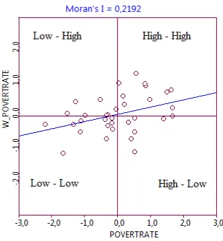
Global Moran Scatter Plot is presented on Figure 2
Figure 2. Moran Scatter Plot of poverty rate in 35 districts
Based on figure 2, Moran’s I = 0,2192, it provide an indication of spatial autocorrelation existence. This is a moderately positive value so there is a positive global spatial autocorrelation. It means that a district with a high poverty rate can be expected to have districts with similar poverty rates around it. So, we continue examine local indicator of spatial association (LISA) values for each district.
Figure 3. LISA Cluster Map of poverty rate in 35 districts
Figure 4. LISA Significance Map of poverty rate in 35 districts
ISSN:2088-5520 C4-67 of poverty rate is spatially influenced by its neighbour.While the one dark blue district is Kab.Semarang where is spatially influenced by its neighbouring districts which have low poverty rate. In contrast, the district of Demak have the light red clasification that indicates spatial outliers, respectively, high value surrounded by low value (HL). Demak which have relatively high value of poverty rate is surrounded by low poverty rate districts. The calculated values of LISA for eight districts are shown on Table I, whereas the others districts have not significant spatial dependency.
TABLE I. CALCULATED LISA’S VALUES OF POVERTY RATE
Districts LISA
Value p-value association
Banjarnegeara 0.81 0.01 High - High Banyumas 0.79 0.01 High - High Cilacap 0.73 0.01 High - High Demak -0.57 0.01 High - Low Kebumen 1.30 0.04 High - High Purbalingga 1.08 0.05 High - High Purworejo 0.03 0.02 High - High Kab.Semarang 0.55 0.03 Low - Low
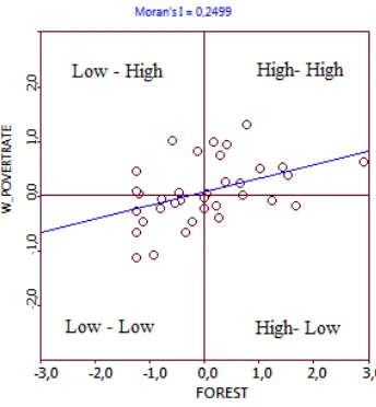
In order to analyze the role of forest in relation with poverty rate, we investigate the spatial autocorrelation between density of forest in each district with poverty rate of each district. The research results are shown on figure 5, 6 and 7 below.
Figure 5. Moran Scatter Plot of forest density and poverty rate in 35 districts
By looking at Moran scatter plot in figure 5, it can be shown that Moran’s I = 0,2499. This is a moderately positive value which means a positive spatial autocorrelation. So there is spatial association between forest density and poverty rate. In details, these properties are presented in figure 6 and figure 7.
Figure 6. LISA Cluster Map of density forest and poverty rate in 35 districts
Figure 7. LISA Significance Map of forest density and poverty rate in 35 districts
ISSN:2088-5520 C4-68 indication of spatial cluster, respectively, low density forest is surrounded by low poverty rate (LL). In other words, density forest is associated with low poverty conditions in neighbouring districts. While the two light blue (LH) districts ,Kebumen and Purbalingga, represent “spatial outliers” condition, wherefore their low density forest are spatially correlated with high poverty rate in surrounding districts. The others have not significant spatial dependency. The detailed values of LISA are shown on Table II below.
TABLE II. CALCULATED LISA’S VALUES OF FOREST-POVERTY RATE
Districts LISA
Value p-value association
Banjarnegara 0.17 0.003 High - High Banyumas 0.38 0.004 High - High Cilacap 1.01 0.003 High - High Demak 1.01 0.008 Low - Low Kebumen -0.1 0.014 Low – High Purbalingga 0.22 0.044 High – High Purworejo -0.59 0.035 Low - High Kab.Semarang 0.1 0.05 Low - Low
Our analysis shows that in the certain districts (Banjarnegara, Banyumas, Cilacap, Demak, Purbalingga and Kab.Semarang), the density of forest has a spatial association with the rate of poverty. Therefore, in those districts, it seems that economic development policy that relate with forest can significantly affect on poverty allevation program.
IV. CONCLUSIONS
The analysis presented in this paper shows that there is some spatial clustering in the distribution of poverty rate in 35 districts of Central Java. In addition, spatial association between forest density and poverty rate occur in some districts of Central Java province.Therefore,by taking policy decisions with these spatial properties can lead to positive development on poverty reduction programs in Central Java province.
ACKNOWLEDGMENT
We would like to express our sincere gratitude to Faculty of Mathematics and Natural Sciences Sebelas Maret University, for providing fund for this research as part of the
SBIR Research Program and to BPS of Central-Java Province for providing poverty data.
REFERENCES
[1] L.Anselin. Spatial Econometrics: Methods and Models. Kluwer Academic Publishers, Dordrecht, The Netherlands, 1988,pp. 16-23. [2] L.Anselin, “Local indicators of Spatial Association-LISA”.
Geographical Analysis 27(2), pp.93-116,1995.
[3] L.Anselin. “The Moran scatterplot as an ESDA tool to assess local instability in spatial association”. In Fischer, M., Scholten, H., and Unwin, D., editors, Spatial Analytical Perspectives on GIS in Environmental and Socio-Economic Sciences, 1996, pp 111-125. Taylor and Francis, London.
[4] L.Anselin, I. Syabri and Y Kho. “GeoDa : An Introduction to Spatial Data Analysis”. Geographical Analysis 38(1), pp.5-22,2006.
[5] BNPB, Peta Indeks Kemiskinan di Indonesia, Badan Nasional Penanggulangan Bencana, 2009, Jakarta, Indonesia.
[6] BPS, Analisis dan Penghitungan Tingkat Kemisikinan 2008, Badan Pusat Statistik, 2008, Jakarta, Indonesia.
[7] BPS, Sensus Penduduk 2010, Badan Pusat Statistik, 2011, Jakarta, Indonesia.
[8] BPS, Jawa Tengah Dalam angka 2010, Badan Pusat Statistik Propinsi Jawa Tengah, 2011, Semarang, Indonesia.
[9] Dinas Kehutanan, Forestry Statistics of Central Java, 2010, Dinas Kehutanan Jawa Tengah, Indonesia.
[10] ESRI Shape files Technical Description, ESRI, 1998, Retrieved 9th. November,2011.http://www.esri.com/library/whitepapers/pdfs/shapefile. pdf.
[11] Griffith, Spatial Autocorrelation and Spatial Filtering, Berlin : Springer-Verlag, 2003, Berlin.
[12] D. Müller, Epprecht, M. and Sunderlin, W.D.“Where are the poor and where are the trees? : targeting of poverty reduction and forest conservation in Vietnam”, Working Paper No. 34, 2006, Center for International Forestry Research, Bogor, Indonesia.
[13] A.Petrucci, Nicola Salvantani. Chiara Seghiere. “The Apllication of Spatial Regression Model to Analysis and Mapping of Poverty”. Environment and Natural Resources Service No. 7, Sustainable Development, FAO,2003,Rome,Italy.
[14] W.D.Sunderlin, Sonya Dewi , Atie Puntodewo, Daniel Müller, Arild Angelsen, and Michael Epprecht. “Why Forests Are Important for Global Poverty Alleviation: a Spatial Explanation”, Ecology and Society
13(2): 24.2008.
[15] SMERU, “ThePoverty Map of Indonesia: Genesis and Significance”,
Newsletter No. 26: May-Aug/2008. SMERU Research Institute, Jakarta, Indonesia.
[16] I.Susanto and Ria Pratiwi,“Using R for Central Java Poverty Modeling with Geographically Weighted Regression” in Proceeding of
International Conference on Open source for Higher Education,
2010,pp.99-103.
[17] E.Yuliasih and Irwan Susanto,”Determining Poverty Map Using Small
Area Estimation Method” in Proceeding of National Seminar on