isprs annals IV 1 W1 67 2017

(1)

UTILIZING THE UNCERTAINTY OF POLYHEDRA FOR THE RECONSTRUCTION OF

BUILDINGS

J. Meidowa∗

, W. F¨orstnerb

a

Fraunhofer IOSB, Ettlingen, Germany - jochen.meidow@iosb.fraunhofer.de b

Institute of Geodesy and Geoinformation, University of Bonn, Germany - wf@ipb.uni-bonn.de

Commission II, WG II/4

KEY WORDS:uncertainty, reasoning, city model, boundary representation

ABSTRACT:

The reconstruction of urban areas suffers from the dilemma of modeling urban structures in a generic or specific way, thus being too unspecific or too restrictive. One approach is to model and to instantiate buildings as arbitrarily shaped polyhedra and to recognize comprised man-made structures in a subsequent stage by geometric reasoning. To do so, we assume the existence of boundary represen-tations for buildings with vertical walls and horizontal ground floors. To stay generic and to avoid the use of templates for pre-defined building primitives, no further assumptions for the buildings’ outlines and the planar roof areas are made. Typically, roof areas are derived interactively or in an automatic process based on given point clouds or digital surface models. Due to the mensuration process and the assumption of planar boundaries, these planar faces are uncertain. Thus, a stochastic geometric reasoning process with statis-tical testing is appropriate to detected man-made structures followed by an adjustment to enforce the deduced geometric constraints. Unfortunately, city models usually do not feature information about the uncertainty of geometric entities. We present an approach to specify the uncertainty of the planes corresponding to the planar patches, i.e., polygons bounding a building, analytically. This paves the way to conduct the reasoning process with just a few assumptions. We explicate and demonstrate the approach with real data.

1. INTRODUCTION

1.1 Motivation

For the representation of urban scenes specific or generic mod-els are conceivable, leading to the classical dilemma of being too unspecific or too restrictive (Heuel and Kolbe, 2001). Spe-cific models comprise object knowledge, for instance about man-made structures, and can therefore directly be related to build-ings. Parametric models, for instance, are often utilized for the representation of buildings although they are unable to represent objects of arbitrary shape. Therefore, buildings of arbitrary com-plexity should be described by generic models. Especially bound-ary representations are suitable representations for polyhedra. In the context of 3D city modeling they are used, but actually often obtained by converting parametric model instances.

Current research directions address the challenge to introduce building shape knowledge without being too restrictive. The de-tection of global regularities can be achieved for instance by clus-tering or hierarchical decomposition of planar elements, followed by a re-orientation and re-positioning to align the patches with the cluster centers, cf. (Zhou and Neumann, 2012, Verdie et al., 2015). Such approaches require specific thresholds and do not exploit the uncertainty of the extracted elements. In (Xiong et al., 2014, Xiong et al., 2015) the topological graph of identified roof areas is analyzed to instantiate and to combine pre-defined low-level shape primitives. Again, parametric models are avoided for the sake of flexibility. The result is a boundary representation with vertical walls and horizontal ground floor.

The instantiation of the building models is based on observations which are inherently uncertain – which holds for automatic and

∗

Corresponding author

semiautomatic acquisitions. This uncertainty results from the measurements, wrong model assumptions, and wrong interpre-tations or inferences. In the context of matching building models with images this issue is pointed out in (Iwaszczuk et al., 2012). Thus a geometric reasoning to detect and to enforce man-made structures should take these uncertainties into account. In (Mei-dow, 2014) the use of pre-defined primitives is replaced by the recognition of man-made structures, i.e., geometric relations be-tween adjacent roof areas. Geometric relations such as orthog-onality or parallelism are found by statistical hypothesis testing and then enforced by a subsequent adjustment of the roof planes.

An automatic reconstruction of buildings is most often derived from airborne laser scanning data or aerial images. This offers the possibility to specify the uncertainty of roof areas: The un-certainty of the planes corresponding to the roof areas is a result of the plane fitting procedure. However, if the input for the rea-soning process is already a generic representation of the build-ing, e.g., an arbitrary shaped polyhedron, the information about the acquisition and its uncertainty is lost since 3D city models usually do not come along with this information. In this case the uncertainties of the planar patches bounding the building have to be derived just from the given boundary representation of the polyhedra. This is the main goal of this paper.

1.2 Contribution

We provide analytical expressions for the uncertainty of planes corresponding to planar patches represented by 3D polygons. These patches bound buildings as provided by 3D city mod-els. By doing so, we consider multiply-connected regions, i.e., polygons or patches with holes, too. Examples are roof areas with openings for dormer windows and buildings with a flat roof around a courtyard.

This contribution has been peer-reviewed. The double-blind peer-review was conducted on the basis of the full paper.

(2)

The approach is based on closed form solutions for the determi-nation of moments for arbitrarily shaped 2D polygons (Steger, 1996b, Steger, 1996a). The idea is to replace the sums over point coordinates occurring in the inverse covariance matrix, i.e., the normal equation matrix, for plane fitting by integrals. This im-plies the assumption that the points are distributed uniformly on the planar patch. We extend this approach to multiply-connected regions and to planar polygons embedded in 3D space. Method-ologically, this is a refinement of the determination of the covari-ance matrix for the centroid representation given a point cloud representing a planar patch (F¨orstner and Wrobel, 2016, p. 397, p. 436).

To demonstrate the feasibility and the usefulness of the approach, we explicate a complete stochastic reasoning process for a build-ing which comprises the determination of the planes’ uncertain-ties, the inference of geometric relations, and eventually the en-forcement of the deduced constraints by adjustment.

2. THEORETICAL BACKGROUND

After clarifying our notation, we present in Section 2.2 the cen-troid representation for planes, the estimation of the correspond-ing parameter values, and the estimation of the accompanycorrespond-ing covariance matrix. For the computation of the normal equation matrix, sums of coordinate moments have to be computed. These sums are then replaced in Section 2.4 by integrals to perform the transition to analytical expressions for the uncertainty of plane parameters given a 3D planar polygon.

2.1 Notation

We denote geometric 2D entities, namely points, with lower-case letters and 3D entities, namely 3D points and planes, with upper-case letters. For the representation of points, planes and transformations we use also homogeneous coordinates. Homo-geneous vectors and matrices are denoted with upright letters, e.g.,xorH, Euclidean vectors and matrices with slanted letters, e.g., xorR. For homogeneous coordinates ‘=’ means an as-signment or an equivalence up to a scaling factor λ6= 0. We distinguish between the name of a geometric entity denoted by a calligraphic letter, e.g.,

x

, and its representation, e.g.,xorx. We use the skew-symmetric matrixS(x)to induce the cross product S(x)y = x×yof two vectors. The operationd= diag(D) extracts the diagonal elements of the matrixDas vectordwhile D= Diag(d)constructs the diagonal matrixDbased on the vec-tord.

2.2 Plane Parameters and their Uncertainty given a 3D Point Cloud

For the representation of an uncertain plane we utilize the cen-troid form, as it naturally results from the best fitting plane through a set of given points. The presentation comprises the cen-troid

X

0where the uncertainty of a point on the plane is smallest, the rotation matrixRfor the transformation of the plane into a lo-cal coordinate system, the maximum and minimum variancesσ2α andσ2

βof the plane’s normal, and the varianceσ2qof the position of

X

0across the plane. Thus the nine parameters compiled in

X0,R;σq2, σα2, σβ2 σα2 ≥σ2β (1)

constitute a convenient representation (F¨orstner and Wrobel, 2016, p. 436).

Parameter Estimation For the estimation of the plane parame-ters we consider the distances of the givenIpoints

X

i,i= 1. . . I to the best fitting plane

A

. Given a point

X

0on

A

, the point-plane distances read

d(

X

i,A) =NT(Xi−X0) (2)

with the plane’s normalNand the points in Euclidean represen-tation. With the squared distances of the least-squares method the objective function is

L = I X

i=1

wd2(Xi,A) (3)

= 1 σ2N

T

I X

i=1

(Xi−X0)(Xi−X0)T

!

N. (4)

We assume independent and identically distributed point coordi-nates with the weightw= 1/σ2 _{for all observations. For the} estimation of plane parameters with individual weights for the points, please refer to (F¨orstner and Wrobel, 2016, p. 436). Set-ting the derivative to zero

∂L ∂XT

0

= 1 σ2N

T

I X

i=1

(−2Xi+ 2X0)

!

N = 0 (5)

reveals that the relation is fulfilled for the centroid

X

0 with the coordinates

X₀= 1 I

I X

i=1

Xi. (6)

For the determination of the plane’s orientation we compute the eigendecomposition of the matrix of second centralized moments

M =

I X

i=1

(Xi−X0)(Xi−X0)T (7)

= RΛRT₌ 3

X

k=1

λkrkrTk (8)

with the three eigenvalues λ1 ≥ λ2 ≥ λ3 in Λ =

Diag([λ1, λ2, λ3])and the orthonormal matrixR= [r1,r2,r3]. The normal of the plane is thenN=r3.

The third eigenvalue is the sum of the squared residuals, thus the estimated variance of the point coordinates can be derived from

b σ2= λ3

I−3 (9)

assuming no outliers are present. If the redundancyI−3is large enough the estimated variance_bσ2_{can be used to fix the weight}

w.

In the following we assume, that the original point cloud data are not available, and only the form of the planar patches is known; hence we need to make assumptions onσ2and the distribution of the 3D points.

Uncertainty Estimation For the specification of the plane’s uncertainty in form of a covariance matrix we centralize and ro-tate the given points in a way that the best-fitting plane for the resulting points isA′ = [0,0,1,0]T_{, i.e., the XY-plane, and the}

(3)

the moment matrix (7). The transformation is achieved by using the centroid

X

0and the rotation matrixR. The covariance matrix is invariant w.r.t. this motion.

In the local coordinate system

Zi′ = q+ tan(α)X angles between the plane’s normal and the Z-axis. With the Jaco-bianJ_i= [1, X′

i, Y ′

i]for each observational equation the normal equation matrix becomes

Please note that the matrixNis diagonal due to the special use of the coordinate system in the centroid, i.e.,

N = Diag ([N11, N22, N33]) (14)

The theoretical covariance matrix isΣ=N−₁

and therefore di-agonal, too. The variances of the estimated parametersq,αand βare

For the reasoning we need the uncertainty of the plane in the global coordinate system as obtained by the transformation given in the next paragraph.

2.3 Centroid representation to homogeneous representation

Given a plane

A

in the centroid representation (1), the homoge-neous representation reads

with the normalNbeing the third column of the rotation matrix Rand the origin’s distanceD = NT_X

0 to the plane

A

. We refer toAhandA0as the homogeneous and the Euclidean part of the homogeneous coordinatesAof the plane. The covariance matrix for the planeA′

= [0,0,1,0]T_{is then}

The point transformationXi=HX ′

iwith the motion matrix

H₌

leads to the plane transformationA=C_A′

with the cofactor ma-trix

ofH_{, see (F¨orstner and Wrobel, 2016, p. 258). Thus the}

covari-ance matrix ofAis

Σ_AA=CΣ_A′A′CT. (23)

In the following we interpret the entries in the normal equation matrix (13) as moments. Assuming a continuous distribution function of the points defining a planar surface patch, we con-sider the moments of arbitrary polygons.

2.4 Moments of Arbitrary Polygons

Assuming that all points in a region have the same weight and are uniformly distributed, the normalized moments of order(m, n) of a regionRare

R. The normalized centralized moments are

µm,n= centralized second moments can readily be computed via

µxx = µ2,0=γ2,0−γ12,0 (26)

µyy = µ0,2=γ0,2−γ02,1 (27)

µxy = µ1,1=γ1,1−γ1,0γ0,1. (28)

Thus it is not necessary to compute these quantities explicitly if the second moments are known (Steger, 1996b).

With the centralized second moments the normal equation matrix (15) can be written as

N=wIDiag([1, µxx, µyy]). (29)

Using the equations for the moments of polygonal regions (Ste-ger, 1996b), we determine the two momentsµxxandµyy. This is done by applying Green’s theorem which allows to replace the area integrals by boundary integrals. By reducing the surface in-tegral to a curve inin-tegral along the borders of the regionR, rep-resented by a polygon

P

, we are able to compute the integral as a function of the polygon’s vertices:

LetP(x, y)andQ(x, y)be two continuously differentiable func-tions on the two-dimensional regionR, and letb(t)be the bound-ary ofR. Ifbis piecewise differentiable and oriented such that the interior is left of the boundary path, an integral over the re-gionRcan be reduced to a curve integral over the boundaryBof

Rin the following manner: Z Z

(4)

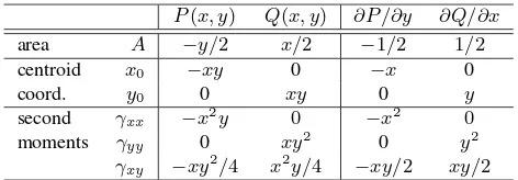
P(x, y) Q(x, y) ∂P/∂y ∂Q/∂x

area A −y/2 x/2 −1/2 1/2

centroid x0 −xy 0 −x 0

coord. y0 0 xy 0 y

second γxx −x2y 0 −x2 0

moments γyy 0 xy2 0 y2

γxy −xy2/4 x2y/4 −xy/2 xy/2

Table 1. Decompositions for the computations of moments fol-lowing (Steger, 1996b).

For polygons, i.e., closed sequences ofKstraight line segments

s

k,k= 1, . . . , K, the parametrization of the segment

s

k(t)is

x(t) =txk+ (1−t)xk−1, t∈[0,1] (31)

with the verticesxkandxk−₁of thek-th segment

s

k(edge). The indiceskare taken cyclically. Thus

Z

b

Pdx+Qdy= K X

k=1

Z

sk

Pdx+Qdy (32)

holds for (30).

For the computation of the integral of the functionF(x, y) = xm_yn

overR, the functionF(x, y)has to be decomposed into ∂Q/∂x and ∂P/∂y according to (30) which cannot be done uniquely. Table 1 summarizes convenient decompositions for the required moments, i.e., the area, the centroid coordinates, and the centralized second moments of the regionR(Steger, 1996b). A decomposition for arbitrary moments can be found in (Steger, 1996a).

Integration and using the decompositions listed in Table 1 yields the following formulas. For details please refer to (Steger, 1996b). The polygon’s area is

A= K X

k=1

Ak with Ak=

xkyk+1−xk+1yk

2 , (33)

taking index addition moduloKinto account. The coordinates of the centroid are

x0 =

1 3A

K X

k=1

Ak(xk+xk+1) (34)

y0 =

1 3A

K X

k=1

Ak(yk+yk+1), (35)

and the second (non-central) moments read

γxx = 1 6A

K X

k=1

Ak x2k+xkxk+1+x2k+1

, (36)

γyy = 1 6A

K X

k=1

Ak yk2+ykyk+1+yk2+1

(37)

γxy = 1 12A

K X

k=1

Ak(xkyk+1+ 2xkyk

+2xk+1yk+1+xk+1yk) (38)

The2×2matrixGof second moments is used in Section 3 to compute a polygons’s orientation in 2D which will then be

trans-formed into the 3D space.

3. APPROACH

Based on the aforementioned concepts, we explicate our ap-proach in detail. After the computation of uncertain planes be-cause of given 3D polygons, we explain the subsequent geometric reasoning consisting of hypothesis generation, statistical testing, and adjustment.

3.1 Uncertainty of Planes

First of all, we determine the plane defined by theK vertices

{X1,X2, . . . ,XK}of the planar polygon embedded in 3D. The plane’s normal vectorAhis (M¨antyl¨a, 1988, p. 218)

Ah= K X

k=1

S(Xk)Xk+1, (39)

here in compact vector representation withXk= [Xk, Yk, Zk]T and index addition modulo K. For boundary representations defining vertex points by the intersection of three or more planes, three non-collinear vertices are sufficient, i.e.,

Ah=S(X3−X1)(X2−X1), (40)

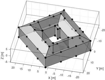
to determine the normal. Figure 1 shows an example where this assumption is violated. Several points are incident to two planes only and hence no vertices.

For the point

X

defined by the mean coordinates X of the vertices1, the incidence

X

∈

A

holds. Expressed in homo-geneous coordinates, this reads XTA = 0with the 3D point X= [X, Y, Z,1]T_{= [U, V, W, T}_]T_{. Thus the plane’s Euclidean}

part ofAreads

A0=−X T

Ah. (41)

To determine the moments of the polygon, we rotate the ver-tices into a plane

A

′′

with Z=const for all points, i.e., A′′ = [0,0,1,−Z]T_{. This can be achieved for instance by means of the}

smallest rotation (F¨orstner and Wrobel, 2016, p. 340)

Q=I₃−(a+b)(a+b)

T

1 +aT_b + 2ba

T_, _a₆₌₋_b

(42)

from vectora= [0,0,1]T_{to vector}_b₌_N _{for the application at}

hand. For horizontal ground floorsN= [0,0,−1]T_{holds and we}

useQ= Diag([1,−1,−1])as rotation matrix. The transformed coplanar points are

X′′k=QTXk with Z ′′

k =Z (43) for all transformed points.

The plane

A

′′constitutes a 2D coordinate system and the poly-gon’s vertices have coordinates(X′′

k, Y ′′

k). We assume the poly-gons to be possibly multiply-connected, i.e., they could enclose holes. Therefore we have to distinguish between exterior and po-tential interior boundaries, often denoted as rings. Figure 1 shows an example from a data set with LoD2-buildings provided by the Magistrat of the city of Linz, Austria (Linz, 2011). The build-ings have been reconstructed by a semiautomatic approach with

(5)

-20

Figure 1. Building with the id 1277 from the Linz data-set. The building’s floor has been modeled by a 2-connected polygon.

standard patterns, based on a digital surface model represented by a point cloud and given building outlines. The building with the ID 1277 features a courtyard, its floor has been modeled by a 2-connected polygon with an exterior and an interior boundary or ring.

WithRrings representing a polygon, the polygon’s area is

A= R X

r=1

Ar (44)

with the signed areasAr according to (33) for each ring. The centroid of the polygon, being the normalized first moment, is

x0= ringrwithKrvertices and edges, and the matrixMof normal-ized second moments contains the elements

µxx=

The matrix of centralized second moments reads

M′′

=G−x0xT0 (49)

and its eigendecompositionM′′

= UΛUT_{yields the}

eigenvec-torsU = [u1,u2]and the two eigenvalues[λ1, λ2] = diag(Λ). Observe, the eigenvaluesλ1andλ2of the2×2matrixM

′′ in (49), derived by integration, correspond to the eigenvaluesλ1andλ2 of the3×3matrixMin (7), derived by summation over all points.

The polygon’s centroid

x

0on the planeA′′= [0,0,1,−Z]T

rep-resented in the 3D space can then be back-transformed via

X₀=Q

to obtain the polygon’s centroid

X

0in the 3D space. And even-tually, the eigenvectorsu1 andu2 in the plane

A

′′

to determine the rotation matrixRas part of the plane’s represen-tation (1).

For the determination of the plane’s uncertainty we consider a virtual scanning process yielding equally spaced points on the plane. Given the areaAof a polygon and a sampling distance∆ in two orthogonal directions, the number of sampling points in the polygon isS = A/∆2_{. Assuming a known, representative} weightw= 1/σ2for all coordinates in (15), we getN11=wS, and therefore, using the eigenvalues ofM′′

in (49)

Obviously, just the productσ∆of the assumed uncertaintyσof the virtual sampling points and the spacing∆has to be specified to compute the complete representation of the uncertain plane

A

corresponding to a given polygon

P

. The uncertain plane in cen-troid representation (1) is completely specified by (50), (51), (52), (53) and (54).

3.2 Geometric Reasoning

For our boundary representation, we assume that each vertex is defined by at least three planes intersecting in one point. Adja-cent faces lying in the same plane will therefore evoke undefined points. Thus in a pre-processing step we check the faces’ binary relations encoded in the given boundary representation for iden-tical planes and merge faces corresponding to the same plane. Beyond that, we restrict ourselves to the relationorthogonality

as the most dominant geometric constraint. For further conceiv-able constraints please refer to (Heuel, 2004) and (F¨orstner and Wrobel, 2016, p. 304ff).

The space of hypotheses is given by all pairs of adjacent faces represented by polygons. For the testing of geometric relations please refer to (F¨orstner and Wrobel, 2016, p. 304ff). Once all potential relations are tested, we have a set of constraints at hand. These result from those hypotheses which could not be rejected by the tests. For the concluding adjustment, a set of consistent, i.e., non-contradicting, and non-redundant constraints is manda-tory since redundant constraints will lead to singular covariance matrices. Since we are dealing with imprecise and noisy observa-tions, we have to face the possibility of non-rejected hypotheses which are contradictory, too. We utilize the greedy algorithm pro-posed in (Meidow and Hammer, 2016) and (Meidow et al., 2009) to select a set of independent constraints automatically.

(6)

4. EXPERIMENTS

For proving the usefulness of the approach we utilize a polyhedral building model which has been instantiated based on an airborne laser scan. Then we derive the uncertainty of the planes corre-sponding to the faces of the boundary representation, perform the geometric reasoning, determine a set of independent constraints, and eventually conduct an adjustment to enforce the inferred con-straints.

Model Instantiation In the data analysis step, the points of the laser scan have been classified into roof and non-roof points. Then the points representing roof areas have been grouped by uti-lizing the RANSAC-based shape detector (Schnabel et al., 2007) provided by the mesh processing software CLOUDCOMPARE.

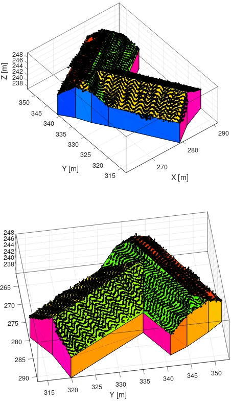
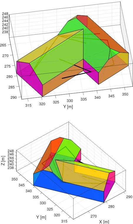
Figure 2 shows points captured by a RIEGL LMS-Q560 scan-ner representing the roof of a farmhouse and a corresponding boundary representation. The reconstruction has been carried out by initially performing a 2D triangulation and computing alpha-shapes to determine the building’s outline. The triangles with points of different planar point groups constitute the boundaries of the roof sections. By analyzing the run of these borders we ob-tained the interior roof structure, i.e., ridge lines, step-edges, and roof valleys. All traversed lines have been simplified by vertex decimation. The solid has been closed by assuming vertical walls on top of the irregularly shaped outline.

The example shows the result of an analysis step, from the point cloud to a polyhedral boundary model. In this paper we do not as-sume the uncertainty of the resulting planar patches to be known. However, we assume the standard deviations, except for a com-mon factor, depend on their form.

As a result, we obtain a generic representation of the building. Only for the non-observed building parts, i.e., the walls and the floor, model assumptions are made. However,the result does not

provide any information about its uncertainty.

Reasoning After the determination of the planes’ uncertainties according to Section 3.1, we determined the set of constraints with a significance level ofα= 0.05(Section 3.2). Very small or thin roof areas are usually very uncertain, too. Therefore, it is likely that hypotheses with these areas involved are not rejected and wrong constraints will be inferred. Thus, we suppress con-straints with faces featuring areas smaller than 16m2_.

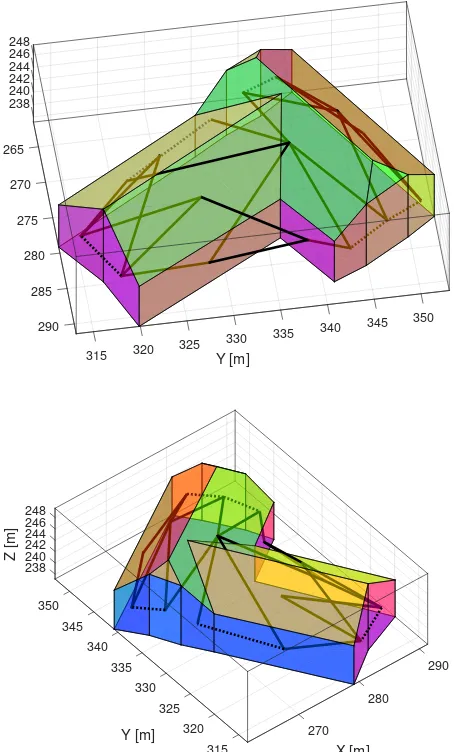
Figure 3 shows the boundary representation of the building with the inferred constraints: 28 times orthogonality and 5 times iden-tity have been detected. The numerous constraints for the ground floor are not visualized for the sake of clarity.

A vertex of our boundary representation is defined by the inter-section of at least three planes defined by the building’s faces. Thus identical or almost identical planes will lead to indeter-mination. Therefore we merge adjacent faces which have been identified to lie in the same plane in a pre-processing step. Fig-ure 4 shows the result of this simplification. After applying the hypothesis testing with the new faces, a set of 20 orthogonality constraints remain.

Some of the inferred 20 constraints are redundant. The greedy algorithm identified a set of 15 independent constraints which are depicted together with the adjusted, i.e., constrained, boundary representation in Figure 5. Now the ridge lines and the eaves are

238 240 242

350 244

Z [m]

246

345 248

340

290 335

Y [m] 330

280

X [m] 325

320 270

315

238 240 242

265 244 246

270 248

275

280

285

350

Y [m]

345 340 335 290

330 325 320 315

Figure 2. Points of an airborne laser scan captured by a RIEGL LMS-Q560 scanner and the deduced boundary representation in two views. The points represent the roof areas of a farmhouse.

horizontal and the building’s outline is rectangular. Of course, the detection and enforcement of further constraints such as identical slopes for the roof areas is conceivable.

5. CONCLUSIONS AND OUTLOOK

We derived analytical expressions for the uncertainty of planes corresponding to the planar patches bounding a polyhedron. This paves the way to stochastic geometric reasoning for generic city models, i.e., the detection and enforcement of man-made struc-tures such as orthogonality, parallelism, or identity, e.g., for groups of buildings.

The estimation of a plane’s uncertainty based on a given point cloud yields a normal equation matrix. Assuming a continu-ous distribution function for points defining a planar patch, we interpret the entries in the normal equation matrix as moments for arbitrarily shaped2 polygons. Furthermore, by considering the signed areas of polygons we are able to cope with multiply-connected polygons, i.e., polygons with interior boundaries defin-ing holes.

(7)

238 240 242

265 244 246

270 248

275

280

285

350

Y [m]

345 340 335 290

330 325 320 315

238 240 242

350 244

Z [m]

246

345 248

340

290 335

Y [m] 330

280

X [m] 325

320 270 315

Figure 3. Derived constraints for the initial boundary representa-tion with 19 faces, depicted in two views. 28 times orthogonality (−) and 5 times identity (· · ·). The numerous constraints for the floor are not depicted for the sake of clarity.

Expectedly, the uncertainty of a plane corresponding to a polygon depends on the polygon’s shape, on its areaA, on the sampling distance∆of the equally distributed virtual sampling points, and on the assumed uncertaintyσfor the coordinates of the sampling points. But just the productσ∆has to be specified and the plane’s uncertainty scales with these factors. For the successful applica-tion of the approach, the specificaapplica-tion of an appropriate, plausi-ble weightw= 1/σ2_{for the sampling point coordinates and the} specification of a sampling distance∆is crucial. Thus future in-vestigations should try to estimate unknown variance factors, too.

For the application at hand, we performed a stochastic geometric reasoning followed by an adjustment of the boundary representa-tion. By considering just the relationsorthogonalityandidentity, already remarkable results are obtained for a real data set: the building’s outline becomes rectangular and the building’s eaves and ridge lines become horizontal.

The method for deriving the uncertainty of geometric entities as-suming pre-specified densities of observations can easily be ap-plied to other estimation problems. For standard configurations

238 240 242

265 244 246

270 248

275

280

285

350

Y [m]

345 340 335 290

330 325 320 315

238 240 242

350 244

Z [m]

246

345 248

340

290 335

Y [m] 330

280

X [m] 325

320 270 315

Figure 4. Two views of the boundary representation after merging adjacent faces with identical planes (13 faces). 20 orthogonality constraints have been detected.

the resulting algebraic expressions not only give insight into the structure of the estimation problem but can be used to replace otherwise unknown information about the precision of geometric entities.

ACKNOWLEDGMENT

The authors would like to thank the anonymous reviewers for their valuable comments and suggestions to improve the quality of the paper.

REFERENCES

F¨orstner, W. and Wrobel, B., 2016. Photogrammetric Computer

Vision. Springer.

Heuel, S., 2004.Uncertain Projective Geometry. Statistical

Rea-soning in Polyhedral Object Reconstruction. Lecture Notes in

Computer Science, Vol. 3008, Springer.

Heuel, S. and Kolbe, T. H., 2001. Building reconstruction: The dilemma of generic versus specific models. KI – K¨unstliche

In-telligenz3, pp. 75–62.

(8)

238 240

265 242 244 246

270 248

275

280

285

350

Y [m]

345 340 335 290

330 325 320 315

238 240 242

350 244

Z [m]

246

345 248

340

290 335

Y [m] 330

280

X [m] 325

320 ₂₇₀

315

Figure 5. Two views of the boundary representation obtained by adjustment of the planes with 15 enforced orthogonality con-straints. As a result the ridge lines and the eaves are horizontal and the building’s outline features right angles.

Iwaszczuk, D., Hoegner, L., Schmitt, M. and Stilla, U., 2012. Hierarchical matching of uncertain building models with oblique view airborne IR images sequences. In: International Archives of the Photogrammetry, Remote Sensing and Spatial Information

Sciences.

Linz, 2011. CC-by-3.0: Stadt Linz – data.linz.gv.at.

M¨antyl¨a, M., 1988.An Introduction to Solid Modeling. Computer Science Press.

Meidow, J., 2014. Geometric reasoning for uncertain observa-tions of man-made structures. In: X. Jiang, J. Hornegger and R. Koch (eds),Pattern Recognition, Lecture Notes in Computer Science, Vol. 8753, Springer, pp. 558–568.

Meidow, J. and Hammer, H., 2016. Algebraic reasoning for the enhancement of data-driven building reconstructions. ISPRS

Journal of Photogrammetry and Remote Sensing114, pp. 179–

190.

Meidow, J., F¨orstner, W. and Beder, C., 2009. Optimal Param-eter Estimation with Homogeneous Entities and Arbitrary

Con-straints. In: Pattern Recognition, Lecture Notes in Computer Sciences, Vol. 5748, Springer, pp. 292–301.

Schnabel, R., Wahl, R. and Klein, R., 2007. Efficient RANSAC for point-cloud shape detection. Computer Graphics Forum

26(2), pp. 214–226.

Steger, C., 1996a. On the calculation of arbitrary moments of polygons. Technical Report FGBV-96-05, Technical University Munich.

Steger, C., 1996b. On the calculation of moments of polygons. Technical Report FGBV-96-04, Technical University Munich.

Verdie, Y., Lafarge, F. and Alliez, P., 2015. LOD Generation for urban scenes. ACM Transactions on Graphics34(3), pp. 30:1– 30:14.

Xiong, B., Jancosek, M., Oude Elberink, S. and Vosselman, G., 2015. Flexible building primitives for 3d building

model-ing.ISPRS Journal of Photogrammetry and Remote Sensing101,

pp. 275–290.

Xiong, B., Oude Elberink, S. and Vosselman, G., 2014. Build-ing modelBuild-ing from noisy photogrammetric point clouds. ISPRS Annals of Photogrammetry, Remote Sensing and Spatial

Informa-tion SciencesII-3, pp. 197–204.

Zhou, Q.-Y. and Neumann, U., 2012. 2.5D Building modeling by discovering global regularities. In:IEEE Computer Society

Con-ference on Computer Vision and Pattern Recognition (CVPR),