REMOTELY-SENSED GLACIER CHANGE ESTIMATION: A CASE STUDY AT
LINDBLAD COVE, ANTARCTIC PENINSULA
K. D. Fieber a *, J. P. Mills a, P. E. Miller b, A. J. Foxc
a School of Civil Engineering and Geosciences, Newcastle University, NE1 7RU, UK - (karolina.fieber, jon.mills)@ncl.ac.uk b James Hutton Institute, Craigiebuckler, Aberdeen, AB15 8QH, UK – [email protected]
c British Antarctic Survey, High Cross, Madingley Road, Cambridge, CB3 0ET, UK - [email protected]
Commission VIII, WG VIII/6
KEY WORDS: Glacier Change, Antarctic Peninsula, Photogrammetry, WorldView-2, Archival Photography, DEM, Surface Matching
ABSTRACT:
This study builds on existing literature of glacier change estimation in polar regions and is a continuation of efforts aimed at unlocking the information encapsulated in archival aerial photography of Antarctic Peninsula glaciers. Historical aerial imagery acquired in 1957 over three marine-terminating glaciers at Lindblad Cove on the West Coast of Trinity Peninsula is processed to extract digital elevation models (DEMs) which are subsequently compared to DEMs generated from present day (2014) WorldView-2 satellite stereo-imagery. The new WorldView-2 images offer unprecedented sub-metre resolution of the Antarctic Peninsula and are explored here to facilitate improved registration and higher accuracy analysis of glacier changes. Unlike many studies, which focus on glacier fronts or only restricted regions of glaciers, this paper presents a complete coverage of elevation changes across the glacier surfaces for two of the studied glaciers. The study utilises a robust least squares matching technique to ensure precise registration of the archival and modern DEMs, which is applied due to lack of existing ground control in this remote region. This case study reveals that, while many glaciers in polar regions are reported as experiencing significant mass loss, some glaciers are stable or even demonstrate mass gain. All three glaciers reported here demonstrated overall mean increases in surface elevation, indicative of positive mass balance ranging from 0.6 to 5.8 metre water equivalent between 1957 and 2014.
1 INTRODUCTION
Globally, mountain glaciers are recognised as a contributor to 20th Century and current sea level rise (Radic and Hock, 2011, Meier et al., 2007). The Antarctic Peninsula can be considered as a mountain glacier system, separate to the Antarctic continental ice sheets, and is comprised of more than 400 individual glaciers. Over the last half century, this region has undergone notable atmospheric warming with an increasing number of positive-degree days (Vaughan, 2006), and various studies have highlighted glacier frontal retreat and advance at selected sites (e.g. Cook et al., 2005). However, there is very little information on mass changes across the Antarctic Peninsula, and the contribution of this region to sea level change is currently poorly understood – e.g. proxy values are used in mass balance compilations (Leclercq et al. 2011). With the Antarctic Peninsula being amongst the most rapidly warming regions globally over last 50 years (Pritchard and Vaughan, 2009), there is an urgent need to explore available data for this region in order to help understand the processes driving glacier mass changes, and subsequent impacts on global sea levels.
Due to the inaccessibility of polar regions related to steep topography, size and remoteness, as well as extreme weather conditions, remote sensing methods are the only practical source of information that can provide observations across extended regions, and enable reliable multi-temporal analysis. Nevertheless, despite the fact that satellite data are now increasingly available for multi-temporal studies, their record is
* Corresponding author
limited and insufficient to identify longer-term climatic trends affecting regions such as the Antarctic Peninsula. However, largely unexplored, historical archives of over 30,000 aerial photographs dating back to the 1940s and 1950s, held by the British Antarctic Survey (BAS), US Geological Survey and Royal Air Force (Fox and Cziferszky, 2008), have recently been scanned to photogrammetric quality and are now more readily accessible. This unique archive represents the only source of information of sub-metre resolution relating to glacier extents and volumes from this earlier period. Photogrammetric techniques can be implemented to explore this archive and enable quantification of Antarctic Peninsula glacier mass change over the last ~60 years.
(g) steep terrain and poor viewing perspectives; (h) limited surface texture, which leads to image correlation difficulties.
In the absence of GCPs measured on the ground (e.g. through classical field survey), introducing control in order to undertake co-registration can be extremely challenging. Some published studies have transferred control from recent GPS-supported aerial photography and airborne LiDAR surveys, but data sources for these methods have a high logistical cost and limited coverage (Fox and Cziferszky, 2008, Barrand et al. 2009, James et al. 2012). Although alternative regional scale datasets can be used to extract ‘proxy’ control points (e.g. digital mapping data, georeferenced satellite imagery), in most cases such data can only offer limited accuracy, and are likely to introduce significant systematic errors. Ultimately, such errors will propagate into subsequent glacier volume change estimation and bias the results (Miller et al. 2009). These difficulties are further compounded in the remote Antarctic Peninsula, which lacks any extended large-scale mapping, and offers only limited coverage through high-resolution satellite imagery.
An alternative to the use of proxy control points is the utilisation of least squares surface matching, a software-based approach which can be used to co-register overlapping digital elevation models (DEMs). This technique has been successfully applied to monitoring of coastal change and geohazards (Mills et al. 2005, Miller et al. 2008) as well as glacial change (Miller et al. 2009, Kunz et al. 2012a). Least squares surface matching is an automated approach which iteratively minimises the differences between overlapping surfaces by point or point-to-surface comparisons, and is able to solve for the unknown transformation model which relates the two DEMs (Kunz et al. 2012a). Nevertheless, this technique requires initial approximate alignment of the two surfaces, which can be performed with the use of (low accuracy) proxy control points.
In this study, the surface matching algorithm developed initially by Mills et al. (2005) for coastal change estimation, subsequently enhanced by Miller at al. (2008) and implemented by Miller et al. (2009) and Kunz et al. (2012a and 2012b) for glacier surface change, is adopted. Miller et al. (2009) and Kunz et al. (2012a and 2012b) both used Advanced Spaceborne Thermal Emission and Reflection Radiometer (ASTER) 15m gridded DEMs as reference data. In contrast to these studies, the research reported here utilises considerably higher resolution WorldView-2 (Digital Globe, 2015a) stereo imagery to produce a ~1m Triangulated Irregular Network (TIN) photogrammetric fixed reference DEM, improving its comparability in terms of spatial resolution to archival photography-derived DEMs.
With the launch of the WorldView-2 satellite in October 2009, imagery of sub-metre resolution and high geolocation accuracy acquired with up to 1.1 day revisit time has become available for the Antarctic region (Digital Globe, 2015a). Imagery of such high spatio-temporal resolution has the potential to revolutionise understanding of the processes taking place in the Antarctic Peninsula by facilitating more accurate registration of datasets from different epochs. Several glacier studies have been conducted with WorldView-2 imagery (e.g. Karimi et al. 2012; Osipov and Osipova, 2015; Racoviteanu et al., 2015; Yavaşlı et al. 2015; Chand et al. in press) focusing on various glaciers around the world, but none have thus far explored the use of WorldView-2 data over the Antarctic Peninsula. Moreover, most of these studies utilised single orthorectified scenes for glacial change analysis rather than stereo-imagery.
Furthermore, unlike most Antarctic Peninsula glacier studies, which have largely focussed only on the frontal parts of the glacier – e.g. 2D glacier frontal retreat or advance (Cook at al. 2005) or frontal elevation changes (Kunz et al. 2012a), this research focusses on quantifying elevation changes across more complete glacier extents. The previous focus on the glacier front is typically a result of the limited coverage of historical photography, which in most cases does not cover the entire glacier extents, as well as a function of the lack of surface texture due to over-exposed imagery and lack of contrast at higher altitudes. In this research it has proven possible to produce complete elevation change maps for two out of three studied glaciers, while approximately 55% of the third glacier was covered. This case study is a prologue to a larger project aimed at analysing ~50 benchmark glaciers located across the Antarctic Peninsula, in order to quantify wide-area ice mass changes over a 60-year period, identifying linkages to regional climate trends and other drivers.
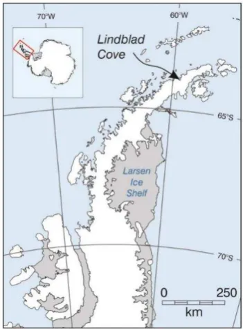
2 STUDY AREA AND DATA 2.1 Study area
The study area is located on the west coast of the Antarctic Peninsula at approximately at 6354’S and 5922’W (Figure 1). The study site covers three glaciers flowing in a north-westerly direction to the south east side of Almond Point, where they enter Lindblad Cove. In the Global Land Ice Measurements from Space database (GLIMS, 2012), all three glaciers are recorded under one ID (G300682E63983S) and one name (McNeile Glacier). However, the World Glacier Inventory (WGI, 2012) distinguishes three glaciers in that area. Only one of them is named, and the remaining two are identifiable only by their WGI ID. Ferrigno et al. (2006) identified those two unnamed glaciers as unnamed Lindblad Cove glacier ‘a’ and ‘b’. McNeile Glacier (WGI ID: AQ7TPE000044) is the most southern, while Lindblad Cove glacier ‘a’ the most northern (WGI ID: AQ7TPE000045). Lindblad Cove glacier ‘b’ is located between the other two (WGI ID AQ7TPE000046). All three glaciers are marine-terminating. To the best of the authors’ knowledge there is no ground field data available for this study site.
2.2 Datasets
Archival Photography: This study utilised aerial photography acquired in the Antarctic summer of 1956/1957 as part of the Falkland Islands and Dependencies Aerial Survey Expedition (FIDASE). In general, and in the context of archival imagery of this era, the quality of the imagery is relatively good, and offers good stereo overlaps, as it was specifically flown for topographic mapping purposes. The FIDASE images were acquired with a Williamson Eagle IX camera with a Ross 6 inch (152 mm) lens and the camera calibration parameters are readily available. The aerial photographs were captured at approximately 1:27,000 scale and were photogrammetrically scanned at 20 µm resolution, providing a ground pixel size of approximately 60 cm.
The imagery covering the Lindblad Cove glacier site was acquired on the 12th and 24th January 1957. Twelve overlapping photographs (two flight lines), taken on 12th January covering the fronts of the three glaciers, were selected for processing (subsequently referred to as “Lower”). A further nine images taken on 24th January were selected to cover the upper part of the same glaciers (“Upper”), as this area was partially obscured by clouds in the 12th January imagery. The images acquired at different dates were initially processed as separate projects to avoid problems with orientation due to e.g. different snow conditions. The image texture and quality of the photography was exceptionally good considering its age.
Satellite imagery: One panchromatic stereo pair of WorldView-2 images (Ortho Ready WorldView-2A stereo imagery product), covering all three glaciers was obtained from Digital Globe (www.digitalglobe.com). The WorldView-2 images were acquired on a single pass on 2nd April 2014. The ground pixel size (~50 cm) was comparable to that of the archival photographs. The quality of the images was generally excellent and geo-referencing information was also provided in the form of Rational Polynomial Coefficients (RPCs). The nominal geolocation accuracy of Ortho Ready standard imagery without ground control is 5 m circular error, 90 % confidence (CE90) (Digital Globe, 2015b), but demonstrated geolocation accuracy is < 3.5 m CE90 (Digital Globe, 2015a).
3 METHODOLOGY
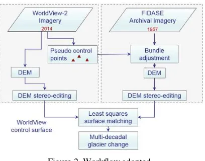
Figure 2 illustrates the workflow used to process the data. WorldView-2 images, provided with orientation information, were used to extract pseudo-GCPs to facilitate initial alignment of archival imagery with contemporary satellite data. This is necessary because while the linear least squares estimate is able to solve for the fine alignment between the DEMs, an approximate initial alignment is required as a starting point to ensure convergence of the solution.
The World-View-2 satellite images were imported into SOCET GXP (BAE Systems, 2015) and visually examined via stereo-viewing. An automatic point matching and relative orientation, using full-covariance strategy, was performed in order to remove existing Y-parallax and provided an RMSE of 0.13 pixel. GCP candidates were subsequently chosen via stereo-viewing of mountainous areas considered to be stable over the years. The XYZ coordinates of these points were recorded. These pseudo-GCPs were then introduced at the absolute orientation stage of the archival photography processing. Different snow cover conditions, as well as different angles of acquisition between the two datasets, rendered the process of transferring the control points non-trivial.
The FIDASE imagery was also processed in SOCET GXP. Interior orientation was carried out by manual measurement of fiducial marks, using the available camera calibration information, followed by automatic tie point measurement. Relative orientation was manually refined and, once satisfactory, the absolute orientation was performed with the help of stereo-viewing, using the full-covariance bundle adjustment strategy within SOCET GXP.
Photogrammetric DEMs were subsequently extracted for both satellite and archival imagery using SOCET GXP Next Generation Automatic Terrain Extraction (NGATE) low contrast strategy as TIN DEMs with approximately 1 m post spacing. Other software offering different image matching techniques could have been tested for DEM generation, however, this was outside the scope of this study. For archival images separate DEMs were generated for each of the two acquisition dates for the lower and upper parts of the glaciers. Due to the nature of the study site and the presence of areas of little or almost no texture, the image matching algorithm sometimes failed to produce satisfactory results both in the case of aerial and satellite imagery. In such regions, DEM points were manually measured in stereo to improve coverage. Gross errors in DEM generation were also manually removed. Subsequently, the DEMs were exported as ASCII files and imported into TerraScan (TerraSolid, 2015) for further processing.
Areas considered to be stable (e.g. rock outcrops, mountain ranges, nunataks) were manually delineated using the Landsat Image Mosaic of Antarctica (LIMA, 2015) and used to clip the WorldView-2 and FIDASE DEMs in TerraScan (TerraSolid, 2015). The spatial resolution of the DEMs was reduced in TerraScan (to approx. 3 m) using the model keypoints classification tool. This avoided excessively long processing times at the surface matching stage, as a substantially reduced surface representation was deemed sufficient to achieve a good quality alignment, and the resultant transformation parameters could then be applied to the full resolution DEMs.
The least squares surface matching algorithm iteratively minimises vertical differences between points in the clipped stable areas on the floating surface (FIDASE) and corresponding patches on the fixed reference surface (WorldView-2). This allows recovery of the seven-parameter 3D Helmert transformation which relates the two surfaces, and this is then applied to the floating surface to precisely align it to the fixed surface (Kunz et al. 2012b). A weighting function based on a maximum likelihood estimator (M-estimator) is included in the algorithm to down-weight potential outlier points, such as those which may be related to gross errors in the DEMs, or related to
minor areas of multi-temporal change, which would otherwise have the potential to bias the solution into an erroneous alignment (Miller at al. 2008).
Once the transformation parameters were obtained for the stable areas, the full resolution FIDASE DEMs (Lower and Upper) were transformed to rigorously align them to the WorldView-2 DEM. The lower and upper DEMs were then combined into one single DEM representing the 1957 epoch. The boundaries of each glacier were then delineated using WorldView-2 stereo imagery and used to clip both datasets. Finally, the differences in elevation and volumetric changes between the two epochs were calculated using LSS software (McCarthy Taylor, 2015). Estimates of mean elevation change as meter water equivalent (m.w.e.) over 57 years were computed according to the following relationship (Hock, 2010):
. �. �. =� ����������
(1)
where � is ice density correction factor, assumed here to be 0.9 (Miller at al., 2009), ������ is the volumetric change in cubic metres and ���� is the total surface area in square metres.
4 RESULTS AND DISCUSSSION 4.1 Archival imagery processing
The results of the initial orientation of the archival imagery in SOCET GXP are summarized in Table 1. In both projects (Lower and Upper) relative orientation was performed using ~100 tie points and yielded RMSE values below 0.5 pixel. Absolute orientation was carried out with the use of evenly distributed pseudo-GCPs (~10-11) transferred from the WorldView-2 project. The RSME in X and Y were below 2 m, while Z RMSE was below 1 m. This is in line with results in Fox and Cziferszky (2008) relating FIDASE aerial photography to GCPs derived from modern GPS-supported aerial photography. The exceptionally good orientation solution is likely a result of the high resolution, good contrast and texture as well as the availability of stereo-pairs rather than a single orthorectified image in both FIDASE and WorldView-2 datasets. The combination of those factors facilitated the accurate identification and transfer of pseudo GCPs and, in consequence, a high quality solution.
Orientation Relative Absolute
RMSE Pixel X [m] Y [m] Z [m] Total [m]
Lower 0.44 1.81 1.80 0.81 2.67
Upper 0.39 1.41 0.93 0.82 1.93
Table 1. Results of relative and absolute orientation of archival photography
4.2 DEM Accuracy
Due to lack of existing GCPs in the study area, it was not possible to assess the absolute accuracy of the DEMs produced by Socet GXP directly. The accuracy of the DEMs was therefore examined by a comparison to manual stereo measurements over the glacier surface, assuming that manual measurements are of higher accuracy than those that have been automatically extracted. It is important to emphasise, though, that this is not an assessment of absolute accuracy (which cannot be achieved without independent GCPs) but a measure of the internal quality of the auto-extracted DEMs.
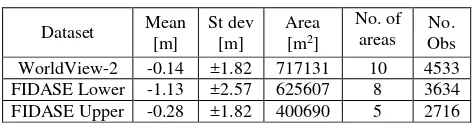
Ten areas of interest of approximately 250 m by 250 m were randomly selected on the glacier surfaces. Mountainous stable areas were excluded due to expectation that steep slopes will lead to poorer results which will not be representative of actual glacier surface quality. Points were manually measured in stereo both in WorldView-2 and FIDASE projects, in a semi-gridded pattern with one point approximately every 10 - 15 m in X and Y. The elevation of those points was subsequently compared to WorldView-2 and FIDASE Lower and Upper DEMs generated by SOCET GXP after initial manual corrections. The results of this comparison are presented in Table 2 and show that on average SOCET-generated surfaces were below manually extracted points.
Table 2. Accuracy assessment of Socet GXP DEMs over glacier areas (comparison to manual measurements in ten areas).
The value of standard deviation is adopted here as the quality measure of the DEMs in the glacier surface areas. In terms of FIDASE DEMs, the higher standard deviation in the Lower project is a result of inclusion of heavily crevassed areas to the front of the glaciers. The overall FIDASE glacier surface DEM accuracy is therefore considered to be the higher of the two estimates (±2.57 m) while for the WorldView-2 glacier surface DEM it is ±1.82 m. Based on error propagation the uncertainty in elevation differences between FIDASE and WorldView-2 glacier surface DEMs was therefore estimated as ±3.14 m.
4.3 DEM Matching
The surface matching was successfully applied to each of the two archive (Lower and Upper) DEMs to align them to the WorldView-2 DEM over selected stable terrain areas. Tables 3 and 4 summarise the elevation difference statistics for Lower and Upper matching results, respectively. The post-match mean difference in both Lower and Upper projects have improved considerably and is closer to 0 m in comparison to the pre-match mean. This suggests that the surface matching algorithm had an impact on removing possible systematic error. The remaining post-match mean difference, in the order of 2.0 - 2.7 m are within the estimated ±3.14 m error in elevation difference. Random checks of sea-level elevations in WorldView-2 and FIDASE DEM showed them to be within 2m of each other.
dh
Table 3. Statistics of elevation differences over stable terrain at Lindblad Cove Lower glacier study site between FIDASE 1957 and WorldView-2 2014 before and after surface matching.
dh
On the other hand, there was little improvement between pre- and post-match RMSE, which confirms that the image orientation stage using pseudo-GCPs derived from WorldView-2 stereo pair was performed particularly well. The initial absolute orientation provided good alignment, which is reflected in small translations and rotations as well as in a stable scale (Table 5).
Parameters Lindblad Cove Lower Lindblad Cove Upper
Tx [m] 0.677 3.536
Ty [m] 1.510 -1.332
Tz [m] 0.285 2.550
Omega [o] 0.008 -0.015
Phi [o] -0.042 0.006
Kappa [o] 0.007 0.014
scale 0.9996 0.9997
Table 5. Transformation parameters for Lindblad Cove Lower and Upper from surface matching algorithm.
The post-matching RMSE of DEM differences over stable (generally rough) terrain of ±17.65 m (the higher of two RMSE of Lower and Upper projects) is similar to the results reported in Kunz et al. (2012a, 2012b). Kunz et al. (2012a, 2012b) however, compared archival DEMs to ASTER DEMs (RMSE ~15 m), therefore data of much lower resolution (15 m), and their pre-match offsets were considerably higher (~ ±50 m). The elevation difference RMSE in this study can most probably be attributed to the rough and steep terrain, and the DEM quality over the significantly flatter glacier surfaces is likely to be considerably higher, and closer to the propagated uncertainty of ±3.14 m reported in Section 4.2. Nevertheless, due to the fact that surface matching will also have an impact on the resultant elevation changes, the true accuracy of those changes should lie somewhere between the two accuracy estimates (between ±3.14 m and ±17.65 m).
4.4 Elevation change
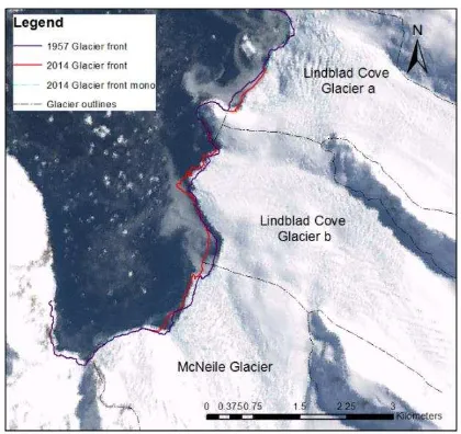
Figure 3 shows the frontal planimetric change of the three glaciers. The glacier fronts were mapped in stereo, in both archival as well as modern satellite image pairs. For completeness, parts of the 2014 coastline were mapped in mono vision, where stereo was not available. The 1957 coastline was subsequently transformed using the parameters listed in Figure 3. While McNeile and Lindblad Cove Glacier ‘b’ fronts have advanced over the 57 years, Lindblad Cove Glacier ‘a’ has partially retreated (south-western part of the coastline). ‘Mono glacier front’ coastline shows that there is some advance of the north-eastern part of the coastline of that glacier. Visual comparison with the Antarctic Digital Database (Ferrigno et al., 2006, http://www.add.scar.org), which includes glacier coastlines from 1956, 1979, 1986, 1989, 1997 and 2000 mapped from various data sources (Figure 4), indicates however that the change in the glacier fronts depends very much on the specific year and has not always showed advance. In fact, according to the database, comparing the 1956 and 2000 coastlines shows retreat for McNeile and Lindblad Cove glacier ‘a’ and partial advance for Lindblad Cove glacier ‘b’. However, it needs to be noted that these mapped historical coastlines may also contain significant error due to differences in the source resolution and quality.
Figures 5 and 6 present the elevation difference maps for McNeile glacier and Lindblad Cove glaciers between 1957 and 2014, respectively. In the case of McNeile glacier the aerial archival photography was either not available or not usable (due to lack of texture, cloud cover, etc.) over the uppermost part of
the glacier, thus that area could not be analysed. Only approximately 55% of McNeile glacier’s area was therefore investigated, as shown in Figure 5. Lindblad Cove glaciers were fully covered with small areas of occlusions in glacier ‘a’ due to cloud cover.
Figure 3. Coastal change of the glaciers between 1957 and 2014 overlain on LIMA mosaic (composed of images
acquired between 1999 and 2003). UTM Zone 21S.
Figure 4. An example of variability in costal changes from 1956, 1979, 1986, 1989, 1997 and 2000 mapped from various data sources in The Antarctic Digital Database (BAS,
2015). Background image is LIMA mosaic. Geographic Coordinate System.
Lindblad Cove glacier ‘a’ is the only glacier displaying some retreat of its front (Figure 3). The elevation change map for Lindblad Cove ‘a’ seems to be the most balanced in the proportion of mass loss and accumulation (balance between yellow and green colours in Figure 6). This is confirmed by the histogram of all elevation change points for Lindblad Cove ‘a’ (over 2 million measurements) in Figure 8. The mean elevation
change in Lindblad Cove glacier ‘a’ is however also positive and yields +1.684 m. Taking into account the uncertainty in elevation changes and the number of observations, the error in the mean is estimated between ±0.004 m and ±0.012 m for this glacier. This example shows that analysis of glacier front advance or retreat alone may sometimes be misleading.
Figure 5. Elevation difference map for McNeile Glacier (AQ7TPE000044). Change from 1957 to 2014. The black
dashed line defines the extents of the glacier mapped in stereo. UTM Zone 21S.
Figure 6 Elevation difference map for unnamed Lindblad Cove glacier ‘a’and ‘b’ (AQ7TPE000045 and AQ7TPE000046). Change from 1957 to 2014. The gap in
the coverage in glacier ‘a’ is due to cloud cover. UTM Zone 21 S.
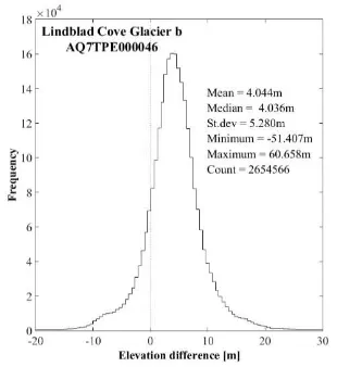
Figure 7. Histogram of elevation differences between archival 1957 and modern 2014 DEMs for McNeile
Glacier (AQ7TPE000044).
Figure 8. Histogram of elevation differences between archival 1957 and modern 2014 DEMs for Lindblad Cove
Glacier ‘a’ (AQ7TPE000045).
Figure 9. Histogram of elevation differences between archival 1957 and modern 2014 DEMs for Lindblad Cove
Finally, Lindblad Cove glacier ‘b’, for which coverage is the most complete and the most uniform, exhibits consistent accumulation towards its front, with elevation changes in the order of + 30 m where the front has advanced, and in the order of + 5-15m further upstream. Some, mostly small, localised elevation losses can be observed in the upper part of Lindblad Cove glacier ‘b’. Figure 9 presents the histogram of all elevation change points (over 2.5 million measurements). The mean elevation change of Lindblad Cove glacier ‘b’ yielded +4.044 m. Taking into account the uncertainty in elevation changes and the number of observations, the error in the mean is estimated between ±0.004 m and ±0.011 m for this glacier.
The standard deviation values for all three glaciers are relatively large and indicate high spread of measured changes across the glaciers. This is to be expected as the changes are not uniform over the glacier surfaces but vary locally. Furthermore, particularly in the case of Lindblad Cove glacier ‘a’, the accumulation of 1.7 m on average is smaller than the surface matching post-match mean. This particular glacier could therefore be considered as relatively stable over the 57 year period.
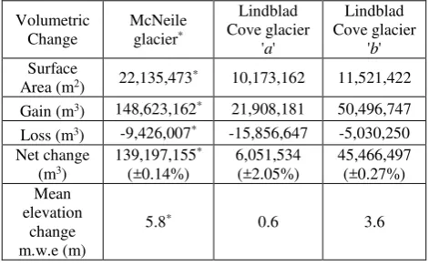
4.5 Volumetric change
The volumetric change, computed between 1957 and 2014 for all three glaciers, is summarised in Table 6. It confirms observations made in the previous section based on elevation maps and histograms of elevation differences. Volumetric analysis was carried out for the complete surface area of the two unnamed Lindblad Cove glaciers and for 55% of McNeile glacier area. The accuracy of net change of each glacier was estimated based on glacier surface area and the higher value of uncertainty in the mean for each glacier.
Despite their similar area, the behaviour of two unnamed glaciers is somewhat different. Lindblad Cove glacier ‘a’, with surface area of 10 million m2, shows relative balance between loss and gain, with net change of +6 million m3 ±2.05 % and mean elevation change of +0.6 m. w. e. over the 57-year period. Lindblad Cove glacier ‘b’, with surface area of 11.5 million m2, displays clear dominance of gain over loss. Its net volumetric gain is 45.5 million m3 ±0.27 % with mean elevation change of
+3.6 m. w. e. over 57 years. The net gain of McNeile glacier is 139 million m3 ±0.14 % with mean elevation change of +5.8 m. w. e. over 57 years. It is important to consider, however, that in the case of McNeile glacier only around 55% of its area was analysed (22 million m2). It is therefore possible that some of the
gain could be balanced out by unmeasured loss in the upper part of the glacier.
5 CONCLUSIONS
This study has presented change estimation between 1957 and 2014 for three glaciers flowing into Lindblad Cove, Antarctic Peninsula. The elevation change estimation was performed using archival FIDASE and modern WorldView-2 stereo imagery of similar spatial resolution, which were used to produce photogrammetric DEMs. Two out of three glaciers were analysed over their full area. Archival imagery was initially orientated with the use of pseudo-GCPs extracted from a WorldView-2 stereo pair, and a least squares matching algorithm was subsequently applied in order to optimise their co-registration, and remove systematic biases. Although, it seems to be in disagreement with the overall trend on the Antarctic Peninsula, all three glaciers studied here displayed elevation and mass increase between 1957 and 2014, which varied from 1.7 to 9.0 m mean elevation increase and from 0.6 to 5.8 m water equivalent, depending on the glacier. Two out of three glaciers exhibited significant mass gain that could not be attributed solely to error in registration.
Least squares surface matching proved to be successful in optimising the registration of two datasets, however, the improvement found in this study was relatively small. This was likely due to the extremely good quality of imagery (high resolution, good texture and contrast) in both datasets, which facilitated very accurate orientation of archival imagery with the use of pseudo GCPs derived from WorldView-2 data. It is anticipated that, due to varying quality of both archival and satellite data over other study sites, the improvement brought about by least squares surface matching will be more considerable at other sites.
This study also showed that the analysis of 2D glacier frontal retreat/advance alone, without the study of elevation change, can sometimes lead to misleading conclusions. Despite exhibiting frontal retreat, one of the glaciers analysed here, showed small accumulation of mass between 1957 and 2014. This gain of mass was, however, within the ‘noise’ of the surface matching, implying that this glacier could be considered stable. Comparison of glacier fronts to data stored in the Antarctic Digital Database (Ferrigno et al., 2006, http://www.add.scar.org) also suggests that this accumulation was not a simple process that happened evenly over the 57-year period, but instead masks considerable short-term fluctuation depending on the year of any particular observations.
ACKNOWLEDGEMENTS
This case study was carried out as part of ‘The spatial and temporal distribution of 20th Century Antarctic Peninsula Glacier mass change and its drivers’ project funded by the Natural Environment Research Council (NERC) – grant number NE/K005340/1.
REFERENCES
BAE Systems, 2015. Socet GXP v4.1 software. User’s Manual.
http://www.geospatialexploitationproducts.com/content/
Barrand, N., Murray, T., James, T., Barr, S., Mills, J., 2009. Optimizing photogrammetric DEMs for glacier volume change assessment using laser-scanning derived ground-control points. Journal of Glaciology, 55 (189), 106-116.
Volumetric
Table 6. Volumetric change between 1957 and 2014. *McNeile glacier volumetric change presented corresponds
Chand, P., Sharma, M.C., in press. Glacier changes in the Ravi basin, North-Western Himalaya (India) during the last four decades (1971–2010/13). Global and Planetary Change. In press.
Cook, A.J., Fox, A.J., Vaughan, D.G., and Ferrigno, J.G., 2005. Retreating glacier fronts on the Antarctic Peninsula over the past half-century. Science, 308 (5721), pp. 541-544.
Digital Globe, 2015a. WorldView-2. Data Sheet. http://global.digitalglobe.com/sites/default/files/DG_WorldVie
w2_DS_PROD.pdf . (Accessed November 2015)
Digital Globe, 2015b. WorldView-2. Digital Globe Core
Imagery Product Guide.
http://global.digitalglobe.com/sites/default/files/DigitalGlobe_C
ore_Imagery_Product_Guide_0.pdf. (Accessed November 2015)
Ferrigno, J.G., Cook, A.J., Foley, K.M., Williams, R.S., Jr., Swithinbank, C., Fox, A.J., Thomson, J.W, and Sievers J. 2006. Coastal-Change and Glaciological Map of the Trinity Peninsula Area and South Shetland Islands, Antarctica: 1843–2001. USGS I-2600-A.
Fox, A.J. and Cziferszky, A., 2008. Unlocking the time capsule of historical aerial photography to measure changes in Antarctic Peninsula glaciers. Photogrammetric Record, 15 (89), pp. 725-737.
GLIMS, 2012. Global Land Ice Measurements from Space and National Snow and Ice Data Center. 2005, updated 2012. GLIMS Glacier Database, Version 1. Boulder, Colorado USA. NSIDC:
National Snow and Ice Data Center.
http://dx.doi.org/10.7265/N5V98602, http://www.glims.org/.
(Accessed October 2015).
Hock R., 2010. Glacier Mass Balance. Summer school in Glaciology Fairbanks/McCarthy 7-17 June 2010. Geophysical
Institute, University of Alaska.
http://glaciers.gi.alaska.edu/sites/default/files/mccarthy/Notes_
massbal_Hock.pdf (accessed November 2015).
James, T. Murray, T. Barrand, N. Sykes, H. Fox, A. & King, M. (2012). Observations of enhanced thinning in the upper reaches of Svalbard glaciers. The Cryosphere 6(6)-1381.
Karimi, N., Farokhnia, A., Karimi, L., Eftekhari, M., Ghalkhani, H., 2012. Combining optical and thermal remote sensing data for mapping debris-covered glaciers (Alamkouh Glaciers, Iran). Cold Regions Science and Technology. 71, 73-83.
Kunz, M., King, M.A., Mills, J.P., Miller, P.E., Fox, A.J., Vaughan, D.G., and Marsh, S.H., 2012a. Multi-decadal glacier surface lowering in the Antarctic Peninsula. Geophysical. Research Letters, 39, L19502.
Kunz, M., Mills, J.P., Miller, P.E., King, M.A., Fox, A.J., and Marsh, S.H., 2012b. Application of Surface Matching For Improved Measurements of Historic Glacier Volume Change in the Antarctic Peninsula. The International Archives of the Photogrammetry, Remote Sensing and Spatial Information Sciences, Melbourne, Australia, Vol. XXXiX-B8, pp. 579-584.
Leclercq, P.W., Oerlemans, J., Cogley, J.G., 2011. Estimating the Glacier Contribution to Sea-Level Rise for the Period 1800– 2005. Surveys in Geophysics, 32, 519-535.
LIMA, 2015. Landsat Image Mosaic of Antarctica
http://lima.usgs.gov/.
McCarthy Taylor, 2015. LSS DTM Software. http://www.dtmsoftware.com/lss-solo/
Meier, M.F., Dyurgerov, M.B., Rick, U.K., O'Neel, S., Pfeffer, W.T., Anderson, R.S., Anderson, S.P., Glazovsky, A.F., 2007. Glaciers Dominate Eustatic Sea-Level Rise in the 21st Century. Science, 317, 1064-1067.
Miller, P.E., Mills, J.P., Edwards, S., Bryan, P., Marsh, S., Mitchell, H. and Hobbs P., 2008. A robust surface matching technique for coastal geohazard assessment and management. ISPRS Journal of Photogrammetry and Remote Sensing, 63 (5), pp. 529-542.
Miller, P.E., Kunz, M., Mills, J.P., King, M.A., Murray T., James T.D. and Marsh, S.H., 2009. Assessment of glacier volume change using ASTER-based surface matching of historical photography. IEEE Transactions on Geoscience and Remote Sensing, 47 (7), pp. 1971-1979.
Mills, J.P., Buckley, S., Mitchell, H.L., Clarke, P., and Edwards, S., 2005. A geomatics data integration technique for coastal change monitoring. Earth Surface Processes and Landforms, 30 (6), pp. 1971-1979.
Osipov, E.Y., Osipova, O.P., 2015. Glaciers of the Levaya Sygykta River watershed, Kodar Ridge, southeastern Siberia, Russia: modern morphology, climate conditions and changes over the past decades. Environmental Earth Sciences, 74, 1969-1984.
Pritchard, H.D., and Vaughan, D.G., 2007. Widespread acceleration of tidewater glaciers on the Antarctic Peninsula. Journal of Geophysical Research, 112, F03S29.
Radic, V., Hock, R., 2011. Regionally differentiated contribution of mountain glaciers and ice caps to future sea-level rise. Nature Geoscience, 4, 91-94.
Racoviteanu, A.E., Arnaud, Y., Williams, M.W., Manley, W.F., 2015. Spatial patterns in glacier characteristics and area changes from 1962 to 2006 in the Kanchenjunga-Sikkim area, eastern Himalaya. Cryosphere 9, 505-523
TerraSolid, 2015. TerraScan software. User’s Manual. http://www.terrasolid.com/products/terrascanpage.php
Vaughan, D.G., 2006. Recent Trends in Melting Conditions on the Antarctic Peninsula and Their Implications for Ice-Sheet Mass Balance and Sea Level. Arctic, Antarctic, and Alpine Research, 38, 147-152.
WGI, 2012. World Glacier Monitoring Service, and National Snow and Ice Data Center (comps.). 1999, updated 2012. World Glacier Inventory, Version 1. Boulder, Colorado USA. NSIDC:
National Snow and Ice Data Center.
http://dx.doi.org/10.7265/N5/NSIDC-WGI-2012-02 (Accessed
October 2015)