______________________ * Corresponding author.
AN ITERATIVE INFERENCE PROCEDURE APPLYING CONDITIONAL RANDOM
FIELDS FOR SIMULTANEOUS CLASSIFICATION OF LAND COVER AND LAND USE
L. Albert *, F. Rottensteiner, C. Heipke
Institute of Photogrammetry and GeoInformation, Leibniz Universität Hannover - Germany (albert, rottensteiner, heipke)@ipi.uni-hannover.de
Commission III, WG III/4
KEY WORDS: Contextual classification, Conditional Random Fields, inference procedure, land use classification
ABSTRACT:
Land cover and land use exhibit strong contextual dependencies. We propose a novel approach for the simultaneous classification of land cover and land use, where semantic and spatial context is considered. The image sites for land cover and land use classification form a hierarchy consisting of two layers: a land cover layer and a land use layer. We apply Conditional Random Fields (CRF) at both layers. The layers differ with respect to the image entities corresponding to the nodes, the employed features and the classes to be distinguished. In the land cover layer, the nodes represent super-pixels; in the land use layer, the nodes correspond to objects from a geospatial database. Both CRFs model spatial dependencies between neighbouring image sites. The complex semantic relations between land cover and land use are integrated in the classification process by using contextual features. We propose a new iterative inference procedure for the simultaneous classification of land cover and land use, in which the two classification tasks mutually influence each other. This helps to improve the classification accuracy for certain classes. The main idea of this approach is that semantic context helps to refine the class predictions, which, in turn, leads to more expressive context information. Thus, potentially wrong decisions can be reversed at later stages. The approach is designed for input data based on aerial images. Experiments are carried out on a test site to evaluate the performance of the proposed method. We show the effectiveness of the iterative inference procedure and demonstrate that a smaller size of the super-pixels has a positive influence on the classification result.
1. INTRODUCTION 1.1 Motivation
Land cover and land use classification are standard tasks in remote sensing that pursue different objectives. Land cover classification focuses on the assignment of land cover labels to (often relatively small) image sites. Land use reveals the socio-economic function of a piece of land, which is typically composed of different land cover elements. The goal of land use classification is to assign a land use label to such pieces of land. In contrast to land cover, land use cannot be derived directly from remote sensing data. Besides spectral characteristics, the composition of different land cover elements within a land use object is important to infer its socio-economic function. For instance, residential land use is typically composed of the land cover elements building, sealed area and grass or trees. Land use classification forms the basis for the verification and update of geospatial land use databases (e.g. Helmholz et al., 2014).
As there is a semantic dependency between land cover and land use, it is reasonable to consider land cover information in the classification of land use. This can be done using a procedure consisting of a sequence of two classification tasks (e.g. Albert et al., 2014a). In a first step, land cover information is derived by a classification of remote sensing data. The second step consists of a land use classification, often segment-based, in which some of the features are derived from the results of the first step. In such a two-step approach semantic relations describing the statistical dependencies between land cover and land use are indirectly introduced to the second classification via additional features derived from the results of the first step.
This strategy for considering contextual information is widely used for land use classification. It is the main drawback of this approach that wrong decisions taken during land cover classification cannot be reversed at later stages. Land cover information directly affects the classification of land use. Thus, wrong decisions taken during land cover classification can easily lead to misclassifications of land use.
Land cover and land use classification exhibit strong contextual dependencies, where context incorporates semantic as well as spatial dependencies between neighbouring sites of land cover and land use classification. In both cases, some classes are more likely to occur next to each other than others. Land use classes typically occur in certain spatial configurations, for instance a
residential area is usually located close to the land use street.
On the other hand, neighbouring land cover sites are likely to belong to the same class, especially if they are small.
We use Conditional Random Fields (CRF) (Kumar & Hebert, 2006) to model the spatial dependencies within each layer. CRF provide a flexible framework for contextual classification. Both layers consist of nodes and edges; they differ with respect to the entities corresponding to the nodes, the employed features and the classes to be distinguished. Both CRFs model spatial dependencies between neighbouring sites, i.e. super-pixels in the case of land cover and land use objects in the case of land use classification. Similar to the two-step approach outlined before, we integrate contextual relations between land cover and land use in the classification process by using contextual features. However, rather than using a two-step procedure, we propose an iterative inference procedure for the simultaneous classification of land cover and land use. During the iterative algorithm, the two classification tasks mutually influence each other, which helps to improve the classification accuracy for certain classes. The approach is designed for input data based on aerial images. Experiments are carried out on a test site and are used to evaluate the performance of the proposed method. The goal is to show the effectiveness of the iterative inference procedure and to investigate the influence of the size of the super-pixels on the classification result.
This paper is structured as follows. Section 1.2 focuses on related work and section 1.3 highlights the contributions of our approach. The methodology is presented in section 2, whereas section 3 describes the experimental evaluation of our approach. Finally, conclusions and an outlook are given in section 4.
1.2 Related Work
There are several approaches for land use classification. They differ with respect to general processing strategy, the extracted features, the classifiers applied and the input data. Some of the approaches apply a two-step processing strategy (Hermosilla et al., 2012; Helmholz et al., 2014). First, a pixel- or segment-based land cover classification is performed. In a second step, the classification results are transferred to the land use objects of a geospatial database. We have presented a two-step land use classification approach using CRF in (Albert et al., 2014a). CRF are applied for land cover as well as land use classification, separately. Both CRFs model spatial dependencies between neighbouring sites, namely pixels in the case of land cover and segments in the case of land use classification. The benefit of considering contextual knowledge in the classification process has already been identified. For instance, for the classification of urban structure types, Hermosilla et al. (2012) incorporate contextual features in land use classification, which describe the relations of land cover areas within a land use object as well as relations between neighbouring land use objects. Contextual features have also been exploited in other fields, e.g. for the classification of 3D point clouds (Xiong et al., 2011).
Instead of implicitly integrating context in the classification process by using contextual features, CRF offer the possibility to model relations between neighbouring image sites as well as relations between image sites at different layers directly, thus, considering context explicitly. There are several multi-layer CRF approaches making use of pair-wise potentials (Kosov et al., 2013; Hoberg et al., 2015; Yang and Förstner, 2011). In our previous work, we have proposed a two-layer CRF for the classification of land cover and land use, where the statistical dependencies between land cover and land use are modelled explicitly by pair-wise potentials (Albert et al., 2014b). However, this limitation to pair-wise potentials is also a major drawback of these approaches. Complex dependencies between more than two variables, like the configuration of several land
cover segments within a land use object, cannot be modelled appropriately in this way. By defining a higher order potential, it is possible to model complex dependencies between more than two random variables explicitly. Higher order potentials have been exploited e.g. for image classification (Kohli et al., 2009). The authors present a class of higher order potentials, referred to as PN-Potts model, which favour individual pixels within a segment to take the same label. Due to the structure of this potential, a solution is found efficiently based on graph cuts. Wegner et al. (2013) applied higher order potentials based on the PN-Potts model for the extraction of road networks from aerial images. In general, inference on higher order potentials is challenging, especially for generic formulations. Standard inference algorithms can effectively approximate a solution for potentials involving only a limited number of variables. In our case, each land use label depends on all spatially overlapping super-pixels, which leads to a generic formulation of higher order potentials involving a large number of variables.
Roig et al. (2011) propose a method to overcome the problem of efficient inference in higher order CRF by using an iterative inference algorithm. In each iteration, they determine a partial solution by minimizing an approximated energy function. The approximation is achieved by replacing the higher order terms by constants, thus, simplifying the higher order potentials to unary terms. As a consequence, the approximated energy function can be minimized using standard inference algorithms. In each iteration, the constants are updated based on the previous partial solution. Their algorithm proceeds iteratively until the energy does not decrease anymore. However, their higher order potentials model quite simple dependencies. In detail, they propose an approach for the simultaneous classification of objects in different views of a scene. Higher order potentials are used to consider occlusions among objects within one view as well as the consistency of the classification result amongst different views.
context features requires a certain degree of knowledge about the characteristics of the contextual relations.
1.3 Contributions
We propose an approach for the simultaneous labelling of land cover and land use, where both classification tasks mutually benefit from each other during inference. A simultaneous classification of land cover and land use is desirable due to naturally inherent relations between both tasks. The integration of these contextual dependencies into classification is supposed to lead to an improvement of the classification accuracy.
In order to solve both tasks simultaneously, so that both classification tasks mutually influence each other, we propose an iterative inference algorithm. It is an extension of the two-step approach proposed in (Albert et al., 2014a), which ties together land cover and land use classification in a principled manner. In our approach, contextual relationships between land cover and land use are modelled implicitly by contextual features. This kind of features provides a better description of the complex statistical dependencies between land cover and land use than it could be realized by pair-wise potentials such as those applied in (Albert et al., 2014b). We use contextual features inspired by Munoz et al. (2010) and Xiong et al. (2011), which take into account the output of the classifier at the other layer. These features have the advantage of considering uncertainties of the class predictions, being based on the beliefs for all classes rather than a single label. In order to model the spatial dependencies within each layer, we apply CRF for land cover and land use classification, respectively. In our previous work, this has been shown to be an appropriate model for that kind of relationship.
The iterative inference procedure is inspired by Roig et al. (2011). In each iteration, we determine the most probable label configuration at each layer separately. Afterwards, the contextual features are updated based on the classification results of the other layer, and, finally, this information is propagated between both layers, resulting in a refined prediction at each layer. Whereas Roig et al. (2011) propagate information by updating the constants related to higher order potentials, we directly update the association and interaction potentials in each CRF after updating the underlying feature values. The update of their higher order potential is exclusively based on the current labelling obtained in the partial solution. In contrast, our approach additionally considers the beliefs for all labels obtained in the partial solutions. The main idea of this approach is that semantic inter-level context helps to refine the class predictions, which, in turn, leads to more expressive context information. The inference procedure is repeated until the classification result does not change anymore.
This paper focuses on the structure of the inference procedure and the design of the contextual features. A main benefit of this approach is that it combines the advantages of a unified model, where uncertainties of class predictions are considered, with the benefit of modelling the complex dependencies between land cover and land use appropriately. Our model tries to determine the most probable label configuration of the two layers simultaneously without taking early decisions. In contrast to the two-step strategy, our approach is able to correct errors made in a previous classification, especially those where a wrong decision is taken with a high uncertainty, i.e. a low belief. For this purpose, the predicted beliefs for all classes serve as input for the extraction of contextual features. Compared to the use of higher order potentials, training and inference are easier,
because algorithms can be simply adopted from the standard CRF and carried out in an iterative procedure.
2. METHODOLOGY 2.1 Conditional Random Fields
Conditional Random Fields were introduced by Kumar and Hebert (2006) for image classification. CRF are undirected graphical models, consisting of nodes and edges . The nodes represent the image sites, e.g. pixels or segments. The edges link adjacent nodes and model statistical dependencies between class labels and data at neighbouring image sites. The class labels of all image sites are combined in a label vector
, … , , … , , where ∈ is the index of an image site and
is the set of all image sites. The goal is to assign the most probable class labels from a set of classes , … , to all image sites simultaneously considering the data . CRF are discriminative classifiers, thus directly modelling the posterior probability | of the label vector given the data :
| 1 , ∙ , ,
. (1)
In equation (1), , are the association potentials and
, , are called the interaction potentials. The association potential , models the relations between class label at site and the observations . The interaction potential
, , models the relations between the labels and of adjacent nodes and the observations . The partition function acts as a normalization constant. The variable refers to the neighbourhood of image site . The parameter determines the weight of the interaction potential relative to the association potential, and, thus, defines the influence of the interaction potential in the classification process. CRF represent a general framework, which allows introducing various functional models for both potentials (Kumar and Hebert, 2006). Thus, one can choose arbitrary discriminative classifiers with probabilistic outputs | for both types of potentials.
2.2 Two-level Graphical Model
2.2.1 Graph Structure: In order to realize a simultaneous classification of land cover and land use, where both classification tasks mutually support each other, we design a graphical model consisting of two separate layers. The layers correspond to hierarchical levels and are arranged one above the other without being connected by edges. We distinguish a land
cover layer and a land use layer. Each layer corresponds to an
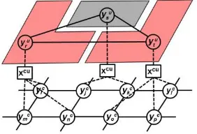
undirected graphical model, which consists of nodes and intra-layer edges. Figure 1 illustrates the design of the two-level graphical model. Inter-level context, i.e. the statistical dependencies of land cover and land use, are modelled via contextual features. These features are derived from the classification results of spatially overlapping image sites in both layers. Inter-level context features form additional observations, which are assigned to all nodes they depend on. We want to estimate the class labels for land cover and land use as random variables for each node i and k in the corresponding layer. The superscript indicates whether the variable belongs to the land cover (c) or land use (u) layer.
geospatial database. The geometry of the image entities remains unchanged during the inference procedure. Examples for the shapes of both sites are shown in figure 2. We use a method proposed by Achanta et al. (2012) for the generation of super-pixels, called Simple Linear Iterative Clustering (SLIC), which is based on an adapted version of k-means clustering. The size and compactness of the generated super-pixels can be controlled by parameters in order to enable a certain adaptation to spectral boundaries in heterogeneous areas. In homogeneous areas, SLIC super-pixels tend to have a compact shape. Land use objects are defined by land use parcels obtained from a geospatial database.
Figure 1. Graphical model consisting of two layers: land cover layer (c) and land use layer (u). Nodes are depicted as circles, intra-layer edges as solid lines, inter-layer observations as rectangles connected to the dependent nodes by dashed lines.
Figure 2. Region images representing super-pixels (left) and land use objects (right). The colours are assigned randomly.
The intra-layer edges model the spatial neighbourhood of each node in the respective layer. The neighbourhood of a node i is composed of its first-order spatial neighbours, i.e. all sites that share a common boundary with the site represented by node i.
We apply CRF according to the notation in equation (1) for land cover and land use classification, respectively. A superscript is added to the variables to indicate whether the variable refers to the land cover (c) or land use (u) classification. The association
potentials c( , x) and u( , x) model the relations between class labels , and the data x. c( , , x) and u( , , x)
represent the intra-layer interaction potentials, which model the spatial dependencies between neighbouring sites within each layer in consideration of the data x.
2.2.2 Association Potentials: The associationpotential predicts how likely node i belongs to a class given the data . The data are taken into account in the form of site-wise feature vectors and for the nodes in the land cover and in the land use layers, respectively. The site-wise feature vectors contain image-based and geometrical features as well as the inter-level context features. Both association potentials take values proportional to the probability of and given the site-wise feature vectors and , i.e. , ∝
for the land cover layer and , ∝
for the land use layer, respectively. We choose the Random
Forest (RF) classifier (Breiman, 2001) for determining the association potentials of both layers. However, each classification is based on a different set of features. RF has proven to be an efficient classifier, also in remote sensing applications (e.g. Schindler, 2012). Some parameters of the RF classifier have to be set beforehand. These are, amongst others, the maximum number of samples used for training, the maximum depth and the number of trees in the forest. Due to considerable differences in the structure of both classification tasks, these parameters have to be selected individually.
2.2.3 Intra-layer Interaction Potentials: This potential models the dependencies of the labels of nodes and being adjacent within one layer, considering the data . The data are taken into account in the form of an interaction feature vector for each edge. We apply the RF classifier for determining the intra-layer interaction potentials of both intra-layers. In contrast to our previous work, we apply a statistical classifier for land cover classification instead of using a potential function favouring a smoothing effect given the data. A pure smoothing of the class labels of neighbouring land use objects as well as land cover super-pixels is not desired. This is true for super-pixels, because the super-pixel segmentation merges pixels with similar characteristics anyway. A statistical classifier favours more probable class configurations given the data. How probable a class relation is, is to be learned from real-world occurrences in representative training data. Thus, the interaction potential is modelled as the joint posterior probability of both labels and given , i.e. , , ∝ , | for the land cover layer, and of both labels and given , i.e.
, , ∝ , | for the land use layer. This corresponds to a standard classification task. Thus, it is possible to handle the interaction potential similar to the association potential by applying, for instance, RF. The difference is that any pair of classes at neighbouring nodes is considered as a single class. In our case, the interaction feature vectors and correspond to the concatenated site-wise feature vectors of two adjacent nodes.
2.3 Iterative Inference Procedure
In the inference step, the most probable label configuration is determined for all nodes in a CRF simultaneously. This is based on maximizing the posterior probability | of the labels given the data. Exact inference is computationally intractable (Kumar and Hebert, 2006). Therefore, only approximate methods can be used. An approximate solution can be obtained by an iterative optimization method based on message passing techniques, e.g. Loopy Belief Propagation (LBP) (Frey and MacKay, 1998). This inference method is applied for the classification in both layers, respectively. However, rather than performing LBP in both layers independently, we apply a joint iterative inference procedure in order to propagate contextual information between both layers during inference.
In the first step of the procedure, a certain number of iterations of LBP are performed at each layer, separately. We obtain partial solutions for land cover and land use by calculating temporary beliefs and inferring a label. The standard LBP algorithms at each layer are then interrupted in order to refine the potentials based on the partial solutions. For this purpose, we update the inter-level context features based on the partial solutions obtained in the first step of the inference procedure. The contextual features model the statistical dependencies of the land cover and land use labels. Their values depend on the temporary beliefs per class label of the partial solution rather than on a single label. These features are calculated based on spatially overlapping image sites, i.e. any node of the land use layer is connected with all nodes from the land cover layer having a spatial overlap with the object corresponding to the land use node. Afterwards, we derive new values for the node and edge potentials at each layer by applying the respective classifier based on the updated site-wise feature vectors. Then, LBP at each layer continues at the point where it was stopped before the update step. The only difference is that node and edge potentials have changed, which affects the further evolution of the messages being passed. The procedure is repeated until a maximum number of iterations is reached. The number of iterations and the number of iterations in each LBP step are set manually based on experience. In the last step of the procedure, the final beliefs are calculated for each node based on the current messages and the node and edge potentials. The label with the maximum belief is assigned to each node.
2.4 Feature Extraction
In our approach, feature extraction is designed for input data derived from high-resolution aerial images, such as digital surface models (DSM), digital terrain models (DTM) and orthophotos. We extract a similar set of features for the nodes of each layer, but referring to different image entities. In the land cover layer, features are extracted for super-pixels. In the land use layer, features are extracted for land use objects, which are defined by the polygonal representation of the GIS-objects of a geospatial land use database. In the following description of the extracted features, the term ‘segments’ refers to super-pixels as well as land use objects. We distinguish three different sets of features: image-based and geometrical features, which remain unchanged during the inference procedure, and contextual
features, which consist of features being updated at each
iteration in the inference procedure. The contextual features are derived from the partial solutions obtained in each step of the inference procedure. The partial solutions provide beliefs for all classes rather than the belief of a single output label.
The set of image-based features consists of spectral, textural and three-dimensional features. The spectral features consist of the mean, standard deviation, minimum and maximum of the normalized difference vegetation index (NDVI), hue, saturation and intensity values, which are estimated from all pixels within the segment. Moreover, we determine the gradient orientations and magnitudes from the intensity image and build a histogram of the gradient orientations weighted by their magnitude per segment. We derive 13 different features from the gradient histogram, for instance the minimum, maximum, mean and standard deviation as well as some ratio values, e.g. the ratio of minimum and maximum values. The textural features are energy, contrast, correlation and homogeneity derived from the Grey Level Co-Occurrence Matrix (GLCM) (Haralick et al., 1973). The GLCM is computed from the co-occurrences of the intensity values of all pixels within each segment. The
three-dimensional features consist of the mean, standard deviation and minimum and maximum values of the height above ground within each segment. The geometrical features are determined from the polygonal representation of the segment. For the land use objects, the polygonal representation is obtained from a geospatial database. For the super-pixels, we use their contours. The geometrical features consist of area, perimeter, convexity, compactness, side ratio of the minimum enclosing rectangle, elongated shape, polar distance, shape index and fractal dimension (Hermosilla et al., 2012). Contextual features encode the inter-level context. For this purpose, we map the classification results to the pixel level, where each pixel is assigned the beliefs per class of the segment-based classification result. Subsequently, we estimate the average of the pixel-wise beliefs per class within each segment:
∑∈∑∈ ∑∈ . (2)
In equation (2), contextual features are calculated per class label ∈ from its respective belief values at the set of all pixels K within each segment. By mapping the land use results to the pixel-level, we can capture the fact that some super-pixels may correspond to more than one land use object. All land use objects having a spatial overlap with the respective super-pixel contribute to the feature calculation according to their degree of overlap. That is also true for the land use layer, where a land use object is typically not totally congruent with its spatially overlapping super-pixels. Furthermore, the number of neighbouring segments is used as a feature. In total, the set of features for the nodes of the land cover layer consist of 48 image-based and geometrical features and 7 contextual features (one per land use class), which are combined in the feature vector for each node . For the land use layer, the feature set contains 48 image-based and geometrical features and 9 contextual features (one per land cover class), which are combined in the feature vector for each node .
2.5 Training
CRF being a supervised classification technique, the parameters of the potentials are learned. In our approach, the association and the interaction potentials are trained separately using representative training data, which implies the training of the RF classifiers. Besides, the user has to define the weights and . They could be determined by a procedure such as cross-validation (Shotton et al., 2009), but this has not been carried out here. Currently, we assign equal weights to both potentials. During the training of the intra-layer interaction potentials, the relations between adjacent nodes are learned. This requires fully-labelled training data for the corresponding layer.
As mentioned before, the classification is based on contextual features. In order to train the classifier appropriately, these features have to be available for the training step. However, the input required for the extraction of contextual features, i.e. the classification result, is not yet available during training. Therefore, an initial classification is carried out as described in section 2.3. The obtained classification results serve as input for the initial estimation of the contextual features.
3. EXPERIMENTS 3.1 Test Data and Test Setup
influence of the size of the super-pixels on the classification result in order to determine a level of detail, which represents a good trade-off between accuracy and computation time. Besides, we compare the results we obtain by applying an iterative inference procedure to the results of the two-step processing strategy presented in (Albert et al., 2014a).
We perform our experiments on a test site in the vicinity of Hameln, Germany. This test area shows various urban, but also some rural characteristics, such as residential areas with detached houses, densely built-up areas, industrial areas, a river, forest, cropland and grassland. The test area has a size of 2 km x 6 km. The input data consist of an orthophoto, a DTM and a DSM derived by image matching. The orthophoto has a ground sampling distance of 0.2 m and consists of four channels (one near-infrared channel, three colour channels). The DSM and DTM provide height information at a resolution of 0.5 m and 5 m, respectively. Furthermore, GIS-objects of the German geospatial land use database forming a part of the Authoritative Real Estate Cadastre Information System (ALKIS®) (AdV, 2008) are used to define the land use objects, which correspond to the nodes in the land use layer. The nodes of the land cover layer correspond to SLIC super-pixels. The segmentation is performed on a three-channel image, where the channels correspond to the difference between the DSM and the DTM (normalised DSM or nDSM), i.e. the height above ground, the intensity and the NDVI extracted from the input data. The use of these three secondary channels instead of the original grey values enables a better adaptation to boundaries of certain land cover segments. We extract SLIC super-pixels of the size of 2,500 and 900 pixels in order to evaluate the influence of the size of the super-pixels on the classification result. The sizes of the super-pixels have been chosen exemplary to represent land cover information in two different levels of details. The SLIC compactness parameter is set to 20 in a range of [1, …, 100], which has been shown in previous tests to allow for a good adaptation to spectral boundaries.
For training and evaluation, reference data are available for both layers. The reference data for the land cover layer consist of pixel-wise reference labels for 37 image tiles, each of size 200 m x 200 m, obtained by manual annotation. The reference data for the land use layer consist of the geospatial land use database for the whole test area, divided into 12 blocks, each of size 1000 m x 1000 m. The reference for each super-pixel is assigned to the most frequent class label among its constituent pixels. However, the simple “winner-takes-all”-strategy for the assignment of the ground truth label to each super-pixel leads to inaccuracies in the training data. In the training process we consider these uncertainties by eliminating uncertain training samples with uncertain class labels, i.e., we only use super-pixels with at least 75% consistent super-pixels as training samples.
We distinguish nine land cover classes (building (build.), sealed
area (seal.), bare soil (soil), grass, tree, water, rails, car, others), and seven land use classes (residential (res.), street, water, railway (rail.), agriculture (agr.), forest, others).
The number of trees and the maximum depth of the RF classifier are set to 200 and 25, respectively, in each case this classifier is applied. The maximum number of training samples serves as bias for classes with less available training samples to ensure that all classes are equally represented during training the classifier. This parameter has to be adapted to the total number of samples available for training. The maximum number of samples is set to 5,000 per class for the association and 1,000 per class for the interaction potentials.The weights
and for the interaction terms are set to 1, thus, the interaction potentials have the same impact on the classification result. Both, the numbers of iterations and are set to 5. The quantitative evaluation is based on cross-validation. For that purpose, the reference data are divided into 12 groups, each consisting of one of the 1 km2 blocks of land use reference data mentioned above combined with spatially overlapping land cover reference data. In each test run, we use one group for the evaluation and all others for training. This is done because the overall number of training samples for land use is quite small. In the 12 test runs, each group thus contributes to the evaluation once. We get a confusion matrix by site-wise comparison of the classification result to the reference for each layer separately; the comparison for the land cover layer is carried out on a per-pixel-basis. The quantitative evaluation is based on the overall accuracy, kappa index, correctness and completeness values derived from the confusion matrix (Rutzinger et al., 2009).
3.2 Results and Discussion
3.2.1 Land Cover Classification: A quantitative evaluation of the results obtained by the iterative inference procedure for two different sizes of the super-pixels is presented in Tab. 1, which also contains the results obtained by the two-step processing strategy presented in our previous work (Albert et al., 2014a).
CRF2-step CRFiterative, 2,500 CRFiterative, 900
Comp.
Table 1. Overall accuracy [%], kappa index [%], completeness (comp.) and correctness (corr.) values [%] for the land cover classes build., seal., soil, grass, tree, water and car obtained by applying the two-step processing strategy (CRF2-step) and the iterative inference procedure based on super-pixels of size 2,500 (CRFiterative, 2,500) and 900 (CRFiterative, 900).
The result of the iterative inference procedure based on super-pixels of size 2,500 yields a mean overall accuracy of about 79.0% and a mean kappa index of 72.8%, which are improved by 2.7% and 3.5%, respectively, for super-pixels of size 900. Compared to the result of the two-step processing strategy, similar accuracy values are achieved by using super-pixels of size 900. This is despite the fact that a class label is predicted for each pixel in the two-step processing strategy, which allows for a higher level of detail. For super-pixels, a class is predicted for all pixels within a super-pixel, although these pixels may belong to different classes. Due to the “winner-takes-all”-strategy in the assignment of a ground truth label to each super-pixel, some classes typically covering only small sets of pixels, such as car, are often merged to other classes, and, thus, are not represented appropriately in the training data. On the other hand, the segmentation of super-pixels merges pixels with homogeneous characteristics, even though some individual pixels may show untypical characteristics. Thus, a smoothing effect of the land cover classification result is achieved, which complies with the naturally inherent characteristics of land cover in the real world. Compared to the result of the two-step processing strategy, the correctness decreases for the classes
building, sealed area and grass and the completeness decreases
completeness and correctness values are improved. For instance, the completeness and correctness for the classes soil and tree are improved by more than 5% in the case of super-pixels of size 900. Both land cover classes benefit considerably from the context information about the present land use class. For the class water completeness and correctness increase by 1.6% and 3.8%, respectively, based on super-pixels of size 900. In contrast, the completeness decreases slightly by 2.2% using super-pixels of size 2,500, but this goes along with a larger increase in correctness compared to super-pixels of size 900. Although the correctness for the class grass decreases, the completeness shows an improvement by more than 2%. The classes rails, car and others show a large increase in correctness along with a large decrease in completeness. The results for the classes rails and others are based on a very small number of samples used both in training and for testing, so that these numbers are hardly representative. The class car is not detected when using large super-pixels due to the lack of detail mentioned before. For the classes building and sealed area, the completeness decreases significantly. This large loss in accuracy may result from the fact that the boundaries of the super-pixels frequently do not match the building and sealed
area boundaries. This is partly caused by inaccuracies in the
DSM and similarities in their spectral characteristics. Smaller super-pixels represent the land cover segments more accurately in a geometric sense, and they can capture more details such as cars or small trees. Larger super-pixels partly cover different land cover classes, which leads to inaccuracies.
3.2.2 Land Use Classification: A quantitative evaluation of the results obtained by the iterative inference procedure for two different sizes of the super-pixels is presented in Tab. 2. For comparison reasons, the results of the two-step processing strategy are also listed there.
CRF2-step CRFiterative, 2,500 CRFiterative, 900
Comp.
Table 2. Overall accuracy [%], kappa index [%], completeness (comp.) and correctness (corr.) values [%] for the land use classes res., street, rail., water, agr., forest and others obtained by applying the two-step processing strategy (CRF2-step) and the iterative inference procedure based on super-pixels of size 2,500 (CRFiterative, 2,500) and 900 (CRFiterative, 900).
The result obtained by the iterative inference procedure based on super-pixels of size 2,500 achieves a mean overall accuracy of 84.8% and a mean kappa index of 74.3%. For super-pixels of size 900, these values stay nearly the same. Compared to the results of the two-step processing strategy, the mean overall accuracy shows a slight decrease by less than 1%. In contrary, the mean kappa index is improved in both cases by approx. 1%. For the classes residential area and street, completeness and correctness do not change significantly compared to the results of the two-step processing strategy. However, the completeness and correctness values are improved for certain classes. For both super-pixel sizes, the class railway shows a large increase in correctness by more than 20% and a smaller improvement in completeness by more than 2%. Furthermore, the correctness increases for the classes water and others by more than 10% and 4%, respectively. However, this goes along with a decrease
in completeness by a similar magnitude for both classes. In contrary, the completeness values of the classes agriculture and
forest are improved by more than 8% and 40%, respectively,
but this goes along with a much smaller decrease in correctness. The largest improvement is obtained for those classes being currently underrepresented in the training data, e.g. forest,
agriculture, water and railway. Due to a lack of available
training samples, these classes benefit the most from additional context information provided by the land cover classification.
3.2.3 Discussion: In the case of land cover classification, the quantitative evaluation shows that reducing the size of the super-pixels has a positive influence on the classification accuracy. By using super-pixels of size 900, we achieve quite a similar level of accuracy compared to the pixel-based land cover classification result obtained by the two-step processing strategy presented in our previous work. Furthermore, the completeness and correctness are improved for certain classes, especially those which cover large, continuous areas in the real world, e.g. forest, agriculture and water. On the other hand, the accuracy for classes covering smaller areas, such as building, decreases. While achieving a similar level of accuracy, the number of nodes and thus the computational effort is significantly reduced by using super-pixels rather than pixels. In the case of land use classification, we also achieve a similar level of accuracy compared to the two-step processing strategy, but the completeness and correctness values are improved for certain classes. The largest improvement is obtained for those classes being currently underrepresented in the training data, e.g. forest, agriculture, water and railway. Although only a few land use objects belong to those classes, the corresponding land use objects cover large parts in the test area.
4. CONCLUSION
We propose an iterative inference procedure for simultaneous classification of land cover and land use. We consider different kinds of context information in the inference procedure. Spatial dependencies are modelled by pair-wise interaction potentials in CRFs for land cover and land use, respectively. The complex statistical dependencies between land cover and land use are modelled implicitly by sophisticated contextual features. The experiments show that the classification results are improved for certain classes compared to the results of a two-step processing strategy (Albert et al., 2014a). Moreover, by using super-pixels rather than pixels, the computational effort is significantly reduced without a significant loss in accuracy. Furthermore, we have shown that reducing the size of the super-pixels has a positive influence on the classification accuracy.
Nevertheless, further enhancements are required in order to improve the classification result. Remaining problems may result from the fact that for some classes we currently have only a low number of training samples, thus, not all classes are properly and equally represented in the training data. Therefore, we want to apply our approach on more test areas with different characteristics and more training data, especially for currently underrepresented classes.
adequate feature selection process, complex dependencies can also be modelled explicitly in a CRF by using higher order potentials. In future work, we aim to investigate whether the statistical dependencies between land cover and land use can be modelled explicitly and probably more appropriately as inter-layer interaction potentials using higher order cliques. This requires a suitable model, which on the one hand, can capture the complex dependencies between land cover and land use, and on the other hand, allows efficient inference.
In our current approach, the number of different land use classes to be discriminated is rather small. In fact, the current class structure corresponds to the coarsest semantic level of the geospatial database. As it is our goal to achieve a very fine semantic resolution of land use classes, further experiments have to be carried out in order to determine the maximum level of semantic resolution which still delivers acceptable results.
Finally, the presented method is the first step of a scheme for updating the given geospatial database. Currently, the geometric delineation of the geospatial objects is assumed to be correct, which might not always be the case. Therefore, we aim to infer changes to the geometric outline of objects automatically, e.g. by splitting and merging objects.
ACKNOWLEDGEMENT
We gratefully thank the Landesamt für Geoinformation und Landesvermessung Niedersachsen (LGLN) and the Landesamt für Vermessung und Geoinformation Schleswig Holstein (LVermGeo) for providing data and support of this project.
REFERENCES
Achanta, R., Shaji, A., Smith, K., Lucchi, A., Fua, P. & Susstrunk, S., 2012. SLIC superpixels compared to state-of-the-art superpixel methods. IEEE Transactions on Pattern Analysis
and Machine Intelligence 34(11), pp. 2274-2282.
Albert, L., Rottensteiner, F., Heipke, C., 2014a. Land Use Classification using Conditional Random Fields for the Verification of Geospatial Databases. In: ISPRS Annals of
Photogrammetry, Remote Sensing and Spatial Information Sciences, vol. II-4, pp. 1-7.
Albert, L., Rottensteiner, F., Heipke, C., 2014b. A two-layer Conditional Random Field model for simultaneous classification of land cover and land use. In: International
Archives of Photogrammetry, Remote Sensing and Spatial Information Sciences, vol. XL-3, pp. 17-24.
Arbeitsgemeinschaft der Vermessungsverwaltungen der Länder der Bundesrepublik Deutschland (AdV), 2008. ALKIS® -Objektartenkatalog 6.0. Available online (visited 16/07/2014): http://www.adv-online.de/AAA-Modell/Dokumente-der-GeoInfoDok/
Breiman, L., 2001. Random Forests. Machine Learning 45, pp. 5-32.
Frey, B. and MacKay, D., 1998. A revolution: Belief propagation in graphs with cycles. In: Advances in Neural
Information Processing Systems, vol. 10, pp. 479-485.
Haralick, R. M., Shanmugan, K., Dinstein, I., 1973. Texture features for image classification. IEEE Transactions on
Systems, Man and Cybernetics 3, pp. 610-621.
Helmholz, P., Rottensteiner, F., Heipke, C., 2014. Semi-automatic verification of cropland and grassland using very high resolution mono-temporal satellite images. ISPRS Journal
of Photogrammetry and Remote Sensing, vol. 97, pp. 204-218.
Hermosilla, T., Ruiz, L.A., Recio, J.A., Cambra-López, M., 2012. Assessing contextual descriptive features for plot-based classification of urban areas. Landscape and Urban Planning 106(1), pp. 124-137.
Hoberg, T., Rottensteiner, F., Feitosa, R. Q., Heipke, C., 2015. Conditional Random Fields for multitemporal and multiscale classification of optical satellite imagery. IEEE Transactions on
Geoscience and Remote Sensing 53(2), pp. 659-673.
Kohli, P., Ladicky, L., Torr, P., 2009. Robust Higher Order Potentials for Enforcing Label Consistency. Int. Journal of
Computer Vision 82(3), pp. 302-324.
Kosov, S., Rottensteiner, F., Heipke, C., 2013. Sequential Gaussian Mixture Models for two-level Conditional Random Fields. 35th German Conference on Pattern Recognition (GCPR), LNCS 8142, Springer, Heidelberg, pp. 153-163.
Kumar, S., Hebert, M., 2006. Discriminative Random Fields.
Int. Journal of Computer Vision 68(2), pp. 179–201.
Munoz, D., Bagnell, A., Hebert, M., 2010. Stacked Hierarchical Labeling. European Conference on Computer Vision 2010, Part VI, LNCS 6316, pp. 57-70.
Roig, G., Boix, X., Shitrit, H. B., Fua, P., 2011. Conditional Random Fields for Multi-Camera Object Detection. IEEE Int.
Conference on Computer Vision 2011, pp. 563-570.
Rutzinger, M., Rottensteiner, F., Pfeifer, N., 2009. A comparison of evaluation techniques for building extraction from airborne laser scanning. IEEE Journal of Selected Topics
in Applied Earth Observations and Remote Sensing 2(1), pp.
11-20.
Schindler, K., 2012. An overview and comparison of smooth labeling methods for land-cover classification. IEEE
Transactions on Geoscience and Remote Sensing 50, pp.
4534-4545.
Shotton, J., Winn, J., Rother, C., Criminisi, A., 2009. TextonBoost for image understanding: multi-class object recognition and segmentation by jointly modelling texture, layout, and context. Int. Journal of Computer Vision 81(1), pp. 2-23.
Wegner, J. D., Montoya-Zegarra, J. A., Schindler, K., 2013. A higher-order CRF model for road network extraction. IEEE
Conference on Computer Vision and Pattern Recognition, pp.
1698-1705.
Xiong, X., Munoz, D., Bagnell, J.A., Hebert, M., 2011. 3-D Scene Analysis via Sequenced Predictions over Points and Regions. IEEE Int. Conference on Robotics and Automation
2011, pp. 2609-2616.
Yang, M. Y., Förstner, W., 2011. A hierarchical conditional random field model for labeling and classifying images of man-made scenes. ICCV Workshop on Computer Vision for Remote
![Table 1. Overall accuracy [%], kappa index [%],iterative inference procedure based on super-pixels of size 2,500 (CRF(comp.) and correctness (corr.) values [%] for the land cover classes completeness build., seal., soil, grass, tree, water and car obtaine](https://thumb-ap.123doks.com/thumbv2/123dok/3215735.1394551/6.595.298.547.335.445/overall-accuracy-iterative-inference-procedure-correctness-classes-completeness.webp)
