MONITORING LAND COVER DYNAMICS AT VARYING SPATIAL SCALES USING
HIGH TO VERY HIGH RESOLUTION OPTICAL IMAGERY
S. J. Lavender a*
a Pixalytics Ltd, Plymouth, United Kingdom - [email protected]
Commission VIII, WG 8
KEY WORDS: Land Cover, Agriculture, Optical, High Resolution
ABSTRACT:
Activities have focused on using the Landsat time-series and Sentinel-2 datasets to monitor land cover dynamics across the United Kingdom, with mapping of specific areas including missions such as Worldview and Kompsat. This short conference paper shows some of the preliminary results from the Landsat Operational Land Imager, Thematic Mapper and Enhanced Thematic Mapper data processing that has included the development of a pre-processing system that includes cloud masking and an atmospheric correction. The results are promising, but further research is needed.
* Corresponding author
1. INTRODUCTION
Human beings benefit from a wide range of goods and services from the natural environment, which are often classified as ecosystem services. Remote sensing has the opportunity to provide data at multiple temporal and spatial scales with landscape indicators, such as vegetation indices, acting as supporting products.
The satellite data will often be a combination of historical archives and new acquisitions, selected to obtain the most current conditions and/or time-series datasets. Therefore, care needs to be taken to reduce differences due to the sensors e.g., waveband specifications and radiometric sensitivity. In addition, there’s also a need to correct for short term atmospheric perturbations through an Atmospheric Correction (AC) and longer term changes due to sensor drift in radiometric performance.
The geometrical (positional) corrections and resulting accuracy should also be judged sufficient that the errors when comparing different images are minimized i.e., if the geometric errors are large then the same position on the Earth may not actually be represented by corresponding pixels in different images.
One of the advantages of the Landsat archive is that a number of corrections have been applied, and the data is supplied in a consistent projection. However, it’s still important to carefully check the type of Level 1 (L1) data being used because different scenes will have different L1 processing levels (Gascon et al., 2015):
- L1T (Standard Terrain Corrected) products are the most accurate level of geometric processing, and free from non-systematic effects.
- L1Gt (Geo Coded and Terrain Corrected) products use a Digital Elevation Model (DEM) to correct parallax errors due to local topographic relief without using Ground Control Points (GCPs) to improve their geolocation accuracy. They exist for
Landsat-7 Enhanced Thematic Mapper (ETM+) products.
- L1G (Systematic Corrected) products are generated when there is a lack of GCPs, and the products are derived purely from data collected by the sensor and spacecraft i.e., the ephemeris data. Therefore, the geometric accuracy will be lower than the L1T products.
1.1 Optical Vegetation Indices
A vast number of terrestrial studies have focused on utilizing ‘greenness’ that’s derived using vegetation indices such as the Normalized Difference Vegetation Index (NDVI). These indices give quantitative measurements of photosynthetically active vegetation through exploiting specific spectral reflectance characteristics; often depending on a high reflectance in the Near InfraRed (NIR) by plant matter contrasting to the strong absorption by Chlorophyll-a in the red wavelengths that’s termed the ‘red edge’ (Curran, 1989). Despite being simplistic, they are often highly correlated with biophysical variables such as the Leaf Area Index (LAI) and because they are a ratio calculation they’re more robust than the more complex algorithms.
However, Clevers (2014) states that the performance of indices is always different and so it’s important to consider the theoretical background validity range and purpose when creating results that are intended to be comparable spatially and temporally. This preliminary research is using NDVI, but the aim is to go on and provide a more complete range of indices once the pre-processing is considered sufficient. For example, the Sentinel-2 (S2) Multi-Spectral Instrument (MSI) provides an opportunity for higher spatial resolution (20 m) vegetation indices and (with its three narrow wavebands in the ‘red edge’ region) more complex algorithms are possible.
The International Archives of the Photogrammetry, Remote Sensing and Spatial Information Sciences, Volume XLI-B8, 2016 XXIII ISPRS Congress, 12–19 July 2016, Prague, Czech Republic
This contribution has been peer-reviewed.
1.2 Choice of Sensors
Activities have focused on using Landsat 8 (L8) and S2 to monitor land cover dynamics across the United Kingdom (UK), with mapping of specific areas including missions such as Worldview and Kompsat. The Operational Land Imager (OLI) on L8 was chosen because it offers a significantly improved spatial resolution compared to medium resolution sensors e.g., the Moderate Resolution Imaging Spectroradiometer (MODIS) and Visible Infrared Imager Radiometer Suite (VIIRS) that have pixel sizes from 0.25 to 1 km. OLI also has high Signal-to-Noise Ratio (SNR) values that are important for mapping surfaces with low reflectances, such as inland waters, because variations can otherwise be lost in the noise.
With S2 MSI data also becoming available, the temporal frequency can be improved as MSI has a higher spatial resolution for the visible / NIR multispectral wavebands (10 m as compared to 30 m) that enhances the fidelity of high resolution features. The revisit time of S2 is 10 days with one unit, reducing to 5 days with two, whilst L8 is a longer 16 days.
There’s also been an analysis of a Landsat TM/ETM+ dataset, from the European Space Agency (ESA) archive, to assess the performance when processing a time-series dataset.
2. METHODOLGY 2.1.1 Landsat Acquisitions
A UK-wide L8 OLI dataset was selected to have minimum cloud cover followed by similar acquisition dates to minimise phenological changes, and hence scene to scene mosaicking discontinuities; see Figure 1. Most of the columns are extracted/calculated from the dataset, but there’s also a comment column for a human assessment of the data quality. This was included because the % of cloud, extracted from the MTL metadata files, may not give a complete indication of the data quality e.g. if there’s thin cirrus cloud that hasn’t been detected.
In total, 289 L8 scenes were selected and downloaded using United States Geological Survey (USGS) Global Visualization Viewer (GLOVIS) with 43 scenes being in the Northern
Figure 1. Example of the OLI dataset selection
In addition to this, imagery is processed from earlier Landsat missions, Landsat 5 and 7 Thematic Mapper (TM) and ETM+ sensors, to provide a time-series of Landsat derived products. This data has primarily come from the ESA Landsat acquisitions, which have been acquired during the last 40 years and are undergoing a reprocessing activity to ensure the data is of the highest possible accuracy (Gascon et al., 2015).
2.2 Pre-processing and Vegetation Index Application The pre-processing starts with a cloud mask, which is calculated using the Automatic Cloud Cover Assessment (ACCA) approach that’s been developed specifically for Landsat data (Irish et al., 2006). Then, the AC is based on an ocean colour ‘dark pixel’ NIR / Shortwave Infrared (SWIR) approach combined with vegetation SWIR ‘dark targets’ (Masek et al. 2006) used to create an water and above-land correction, respectively (Lavender, 2014). The focus has been on making the AC operationally robust, which aids the choice when multiple solutions are considered equally valid. When sensors have no SWIR waveband, especially for missions like Kompsat-2 and -3 where there are only 4 wavebands, the aerosol component is significantly simplified and the option of just a Rayleigh correction is tested. For simplistic band-ratio algorithms, such as NDVI, the assumption is that the algorithm itself is relatively insensitive to any remaining atmospheric artefacts.
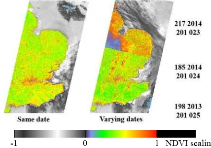
As an initial step, the L8 dataset has been processed using a cloud-based infrastructure to create a UK-wide mosaic that provides the baseline mapping. Figure 2 shows the results of mosaicking L8 scenes processed to NDVI; in this case without the cloud mask applied. When the data is available from the same date (as shown on the left) the edges are seamless, but when different dates are used the influence of phenology dominates.
-1 0 1 NDVI scaling
Figure 2. Mosaicking Landsat 8 scenes from the same date (left) and differencing dates (right, with the day of year / year and path / row listed for each of the three scenes). The colour bar underneath shows how the NDVI values are mapped: shades of
grey for negative values and then blue to green to yellow to orange to red for positive values.
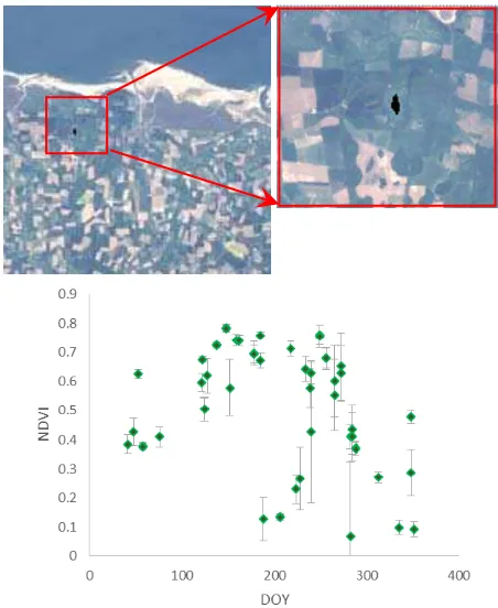
As a second example, Landsat 5 TM and 7 ETM+ imagery has been processed with ACCA cloud filtering, to remove cloud contaminated pixels, and then a Rayleigh correction to reduce the atmospheric effects. Figure 3 shows the area being analysed, which is situated near the northern coast of East Anglia within the UK, with a polygon of pixels corresponding to a grassland area being plotted.
In the plot (Figure 3 bottom) the data from all years has been plotted together, with the x-axis being the Day of Year (DOY), and so the overall shape follows the phenology with year-to-year variations in NDVI being influenced by temperature and rainfall. The errors bars are showing the variability within the polygon as the plot is of the mean and standard deviation. For The International Archives of the Photogrammetry, Remote Sensing and Spatial Information Sciences, Volume XLI-B8, 2016
XXIII ISPRS Congress, 12–19 July 2016, Prague, Czech Republic
This contribution has been peer-reviewed.
the majority of the points this variation is small, but for some images it is significant indicating that there’s a potential error source e.g. cloud shadows or thin cirrus cloud.
Figure 3. Landsat 5 TM and 7 ETM+ dataset shown as the area under investigation (top left), zoomed in to show the polygon being extracted (top right). There’s also (bottom) a plot of the
mean NDVI values versus the DOY where the error bars indicate the variability within the polygon.
3. CONCLUSION
The AC within the pre-processing is showing promising results, but there are several areas where the AC approach can be
technically improved e.g.
- Geometry of each pixel needs to be calculated more accurately
- Run the AC with daily, rather than climatological, auxiliary information (such as air pressure and water vapour concentration).
- Work is needed on cloud shadow correction as only cloud pixels are currently removed
- No correction for bidirectional reflectance (BRDF) effects is currently applied
In addition, if a UK-wide seamless mosaic is needed a phenology adjustment will have to take into account the effects of temperature and rainfall or be based on statistics / image matching. A phenological model is currently preferred, as a physical basis for the results will be maintained, but may provide a more variable result.
Work has started on the S-2 MSI data, but the AC results are still being analysed and optimised.
ACKNOWLEDGEMENTS
This research has been funded internally by Pixalytics Ltd, with knowledge gained by Dr Lavender’s consultancy involvement in the ESA IDEAS+ (Instrument Data quality Evaluation and Analysis Service) project. The Landsat data is courtesy of USGS/NASA for Landsat-8 and USGS/ESA/NASA for the earlier Landsat missions.
REFERENCES
Clevers, J.G.P.W. 2014. Beyond NDVI: Extraction of biophysical variables from remote sensing imagery, in Land
Use and Land Cover Mapping in Europe: Practices and Trends,
Springer-Verlag, Berlin Heidelberg.
Curran, P.J. 1989. Remote sensing of foliar chemistry. Remote
Sensing of Environment, 29, pp. 271-278.
Gascon, F., Biasutti, R., Ferrara, R., Fischer, P., Galli, L., Hoersch, B., Lavender, S., Meloni, M., Mica, S., Northrop, A. Paciucci, A., Saunier, S. 2015. Bulk processing of the Landsat MSS/TM/ETM+ archive of the European Space Agency. SPIE 9643, Image and Signal Processing for Remote Sensing XXI
(October 2015).
Irish, R.R., Barker, J.L., Goward, S. N. and Arvidson, T. 2006. Characterization of the Landsat-7 ETM automated cloud-cover assessment (ACCA) algorithm, Photogramm. Eng. Remote
Sens., 72(10), pp. 1179-1188
Joshi, N., M. Baumann, A. Ehammer, R. Fensholt, K. Grogan, P. Hostert, M.R. Jepsen, T. Kuemmerle, P. Meyfroidt, E.T.A. Mitchard, J. Reiche, C.M. Ryan, & B. Waske, 2016. A Review of the Application of Optical and Radar Remote Sensing Data Fusion to Land Use Mapping and Monitoring, Remote Sensing,
8(70).
Lavender, S.J., 2014. Multi-sensor ocean colour atmospheric correction for time-series data: Application to LANDSAT ETM+ and OLI data, EARSeL eProceedings, 13(2), pp. 58-66.
Masek, J.G., E.F. Vermote, N. Saleous, R. Wolfe, F.G. Hall, F. Huemmrich, F. Gao, J. Kutler, & T.K. Lim, 2006. A Landsat surface reflectance data set for North America, 1990-2000,
Geoscience and Remote Sensing Letters, 3, pp. 68-72
Revised May 2016
The International Archives of the Photogrammetry, Remote Sensing and Spatial Information Sciences, Volume XLI-B8, 2016 XXIII ISPRS Congress, 12–19 July 2016, Prague, Czech Republic
This contribution has been peer-reviewed.