POINT CLOUD METRICS FOR SEPARATING STANDING ARCHAEOLOGICAL
REMAINS AND LOW VEGETATION IN ALS DATA
R. Opitz a* and L. Nuninger b*
*
Corresponding author. a
CAST, University of Arkansas, Fayetteville, AR USA / LEA ModeLTER / MSHE Ledoux USR 3124, UFC, Besançon, France – [email protected]
b Chrono-Environnement UMR 6249 / LEA ModeLTER / MSHE Ledoux USR 3124, CNRS, Besançon, France –
Commission xx, WG xx/x
KEY WORDS: ALS, classification, archaeology, built structures, terrain models
ABSTRACT:
The integration of Airborne Laser Scanning survey into archaeological research and cultural heritage management has substantially added to our knowledge of archaeological remains in forested areas, and is changing our understanding of how these landscapes functioned in the past. While many types of archaeological remains manifest as micro-topography, several important classes of features commonly appear as standing remains. The identification of these remains is important for archaeological prospection surveys based on ALS data, and typically represent structures from the Roman, Medieval and early Modern periods. Standing structures in mixed scenes with vegetation are not well addressed by standard classification approaches developed to identify bare earth (terrain), individual trees or plot characteristics, or buildings (roofed structures). In this paper we propose an approach to the identification of these structures in the point cloud based on multi-scale measures of local density, roughness, and normal orientation. We demonstrate this approach using discrete-return ALS data collected in the Franche-Comte region of France at a nominal point density of 8 pts/m2, a resolution which, in coming years, will become increasingly available to archaeologists through government supported mapping schemes.
1. INTRODUCTION
1.1 Standing archaeological remains in mixed scenes
The integration of Airborne Laser Scanning (ALS) survey into archaeological research and cultural heritage management has substantially added to our knowledge of archaeological remains in forested areas, and is changing our understanding of how these landscapes functioned in the past. To date, the majority of the remains identified through ALS can be characterised as earthworks- slight or sometimes substantial local variations in micro-topography (Opitz and Cowley, 2013). While many types of archaeological remains manifest as micro-topography, several important classes of features commonly appear as standing remains. The identification of these remains is important for archaeological prospection surveys based on ALS data and typically represent structures from the Roman, Medieval and early Modern periods. They are essential to the characterization of the site distribution and landscape organization of these periods.
Standing archaeological remains are frequently found in areas characterized by dense low vegetation. The identification of these remains has been particularly problematic in the analysis of ALS data collected for Mediterranean landscapes (Lasaponara and Masini, 2009; Opitz, 2009), and is also relevant in temperate European landscapes. Standing structures in mixed scenes with vegetation are not well addressed by standard classification approaches developed to identify bare earth (terrain), individual trees or plot characteristics, or buildings (roofed structures). These structures are typically mixed into the low- or medium- vegetation classes by
terrain-seeking algorithms, and into ‘understory’ by vegetation characterizing algorithms, and are classified as vegetation by building-extraction algorithms. While full-waveform lidar data provides a relatively straightforward path to distinguishing these structures from the surrounding vegetation based on echo-width filtering (Doneus et al., 2008), the substantial archive of discrete return ALS data must be treated using purely geometric measures, as described below.
2. METHODS AND ALGORITHMS
2.1 Related Approaches to Mixed Scenes
2.1.1 Multi-scale Segmentation of Terrestrial Laserscans (TLS) of Natural Scenes:
TLS scans of natural scenes that contain multiple elements, including vegetation, stones, and soil, pose many of the same problems as mixed natural scenes in ALS, including
heterogeneity in the morphological characteristics of each class of features, random orientation of structural elements, and local shadow effects in the point cloud. Consequently the
fundamentals of the approaches developed to segment scenes are similar. The approach developed by Lague et al. (2012, 2013), like the one presented here, uses a measure of multi-scale dimensionality to characterize the local geometry of the neighbourhood around each point. They develop a metric for multi-scale dimensionality based on the dimensionality of a local neighbourhood sphere at varying scales s around each point. They describe dimensionality at each scale using the variance in the eigenvalues of the first three components of the PCA of the points in each sphere. The dimensionality measures
at multiple scales are combined in the final classification. They develop a semi-automatic approach, in which a classifier is trained and then deployed over a larger scene. While Lague et al.’s approach uses PCA to describe dimensionality – the extent to which the point cloud geometry is 1D, 2D, or 3D, our approach uses roughness, point density, and normal orientation. The ideal measure of dimensionality to characterize 3D point clouds is a matter of debate. Fractal dimensionality and multifractal measures (e.g. Wendt et al., 2007) and spatial correlation measures (e.g. Sim et al., 2010) have been used successfully on TLS data. In our approach the combination of roughness, density and normal orientation is preferred for distinguishing between approximately planar features (walls) and surrounding amorphous points (understory canopy) at relatively coarse resolutions compares to typical TLS data.
Measures of roughness (e.g. Vetter et al. 2011), density (e.g. Ferraz et al. 2010) and normal vector (e.g. Dorninger and Nothegger 2007) are all regularly used to segment point clouds. The originality of our approach is in combining the measures, and iteratively calculating them across multiple scales in what is essentially an opening operation. The application to standing archaeological remains in mixed scenes is also, to the extent of the authors’ knowledge, original.
2.1.2 Hierarchical Segmentation of ALS of Urban Scenes:
The urban scene problem differs from natural scenes in that many target objects e.g. roofs and building walls are approximately planar and not immediately surrounded by other returns, and in that vegetation is often in the form of individual or small groups of trees, without the presence of an understory. Successful approaches to urban scene segmentation include wavelets (e.g. Keller and Borkowski, 2011), region growing (e.g. Forlani et al. 2006) and RANSAC (e.g. Niedhart and Sester, 2008).
2.2 Description of the proposed method
In this paper we propose a method to segment ALS point clouds representing mixed scenes containing returns from terrain, vegetation, and standing archaeological remains using purely geometric measures. This method has been developed using ALS data at a nominal density of 8 pts/m2, a resolution likely to become increasingly available to researchers and managers through regional and national mapping schemes. In the proposed approach a point cloud representing a mixed scene containing terrain, vegetation and standing archaeological remains is selected for analysis. The point cloud is initially classified using a terrain-seeking algorithm, in this case a custom macro implemented in Terrascan. Terrascan relies on an adaptation of Axelsson’s algorithm, which discriminates between terrain and vegetation points using a series of adaptive TINs (Axelsson, 2000). This algorithm is well suited for large scale terrain/non-terrain segmentation of point clouds, but significantly less well suited to identifying individual components within the vegetation segment of the point cloud. The pre-classified point cloud is then segmented on the basis of three criteria: roughness, density, and normal orientation. All roughness calculations are performed in CloudCompare, and density and normal calculations are performed in Meshlab. Regions of points representing standing remains, which were initially identified as vegetation by the Terrascan algorithm, are reclassified on the basis of their low roughness and consistent normal orientation, as calculated at multiple scales.
The proposed method has several advantages. First, computation is relatively rapid, because the 3D point cloud is treated directly and interpolation is avoided. Further, it is implementable using basic point cloud morphology metrics, meaning it can be carried out using a variety of open source software packages. Finally, only a few parameters need to be tested and set. Consequently, this approach can be implemented and adapted by researchers with limited computing resources, making it widely accessible.
2.2.1 Multi-scale iterative roughness calculations: In the first stage of the analysis local roughness values are calculated for each point at a scale s1. The roughness calculation is basic: at each point the roughness is calculated as equal to the distance between the point and the least square best fitting plane computed on its nearest neighbours. Points with fewer than 3 nearest neighbours within the sphere defined by the scale of the analysis are assigned an invalid scalar value (NaN) (CloudCompare, 2012). The Weibull distribution of the roughness values is calculated and points falling within one and two standard deviations (σ) of the distribution are identified
(figure 1). Points with roughness values exceeding 1σ of the
roughness distribution are removed. Roughness values are then recalculated on the modified point cloud on a smaller spatial scale s2 and points exceeding 1 σ are again removed. In the
third pass, the roughness values are recalculated on a larger scale s3. For ALS data at nominally 8 pts/m2 and archaeological features at the 1-5m scale, s1 is set at 5m. The parameters s1, s2 and s3 should be varied with respect to the scale of the standing remains sought and the nominal point density of the ALS data. For the case studies here, these parameters were set at 5, 3 and 11m. The selection of appropriate scale parameters is essential for the identification of standing architecture, and successful segmentation. If objects of significantly different scales are present, the segmentation procedure would need to be performed repeatedly to ensure capture of objects across scales.
Figure 1: The distribution of roughness values the scale of 5m. The 1σ and 2σ cut-off points are indicated by red vertical lines.
2.2.2 Segmentation on local density: After initial segmentation of the point cloud based on multi-scale roughness, some points classified as vegetation remain in the scene. In the case studies here, these are clearly distinguishable by local point density. Local point densities are calculated on a 3x3x3 matrix of neighbours, and areas with low point densities, typically beyond 2σ in the distribution, are excluded. In the first two
examples shown here, the use of a 3x3x3 matrix of neighbours produces good results. At other scales, it may be appropriate to vary the size of the neighbourhood. Optionally, a second pass of density segmentation may be undertaken, varying the size of the neighbours matrix.
2.2.3 Segmentation on normal orientation: After segmentation on local density remaining components can be separated into individual walls, and walls distinguished from terrain and any remaining vegetation components on the basis of normal orientation. Normal orientations are calculated for the resulting point cloud on the basis of each point’s neighbours (26 neighbours are used in these calculations, representing a 3x3x3 matrix without a preferred orientation). The normal orientations are also used to differentiate between multiple structures at different orientations in the scene, on the basis of dominant normal orientation. As with local point densities, a second pass may be needed if features at substantially different scales are present in the scene.
2.3 Intended Applications
Archaeological sites on which standing remains may be expected are often identified in ALS data on the basis of more easily detected and visualized microtopographic features, e.g. mounds, ditches, cuttings, or platforms. This approach is intended for the analysis of forested scenes, where the potential for standing structures has been established. Consequently, the sites assessed for this paper are relatively small (under 1 ha.). This approach could be scaled up to address larger areas, but the problems of doing so, notably increased computational expense, are not addressed here.
3. CASE STUDY SITES
The approach developed to identify standing remains was tested at three sites with known standing structures. Two of these sites, Montfaucon and Bregille, contain substantial preserved walls, and the dominant scale of the standing archaeological features is 2-5m. At the third site, Chapel de Buis, the dominant scale of standing features is 0.25-1m. All three sites were characterized by mixed deciduous forest with medium to dense understory canopies.
3.1 Montfaucon
The remains of the chateau and village of Montfaucon are located in mixed deciduous forest. In this sample scene a single long wall, preserved to more than 2m in height and less than 1m in width is present (figure 2).
Figure 2. The sample area at Monfaucon. More vegetation was present at the time of ALS data collection.
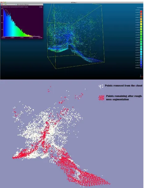
3.1.1 Calculations: Roughness values for the entire point cloud are calculated at the 5m scale (figure 3- top). The distribution of roughness values is calculated and points exceeding 1 σ of the distribution are classified as vegetation and
removed from subsequent segmentation iterations. The scene is subsequently segmented at 1 σ at 3m and then 11m scales.
After the roughness segmentation, some vegetation points remain (figure 3- bottom).
Figure 3(top) 5m roughness values in the Montfaucon scene, viewing the main wall end-on. (bottom) Points remaining after the roughness segmentation phase (red) seen within the point cloud (white).
Local point densities are calculated for the resulting point cloud and final remaining vegetation components, characterized by low point densities (green points, figure 4), are removed. Areas with consistent normal orientations (figure 4) define regions of terrain and standing architectural remains. Terrain regions are confirmed by checking against the initial Terrascan
classification of the point cloud. The resulting point cloud contains three classes: terrain, standing remains, and vegetation (figure 5).
3.2 Bregille
A ruined building with multiple walls standing to heights of more than 2m, and averaging 50cm in width, provides a second case study. In this case several walls are present, at different orientations. The remains at Bregille are, as for the Montfaucon scene, initially segmented based on roughness values, iterating over the point cloud at scales s1=5m, s2=3m, and s3=11m. The results of this step can be seen in figure 6. Two vegetation components remain (figure 7). The local density values for the remaining points are calculated, and points with density values falling outside 2 σ of the density distribution are classified as
vegetation and removed. At this point only returns from the terrain and the standing remains are present in the point cloud.
Figure 4. Points coloured by density and normal represented as vectors. Remaining vegetation points are characterized by coherent normal, but low local densities.
Figure 5. Final segmentation into terrain areas (white), standing remains (pink) and vegetation (green).
Terrain points, as identified in the initial Terrascan classification, are removed and the standing remains can be segmented into individual walls based on normal orientation (figure 8). Some misclassified terrain points remain (red points, figure 8) after the density segmentation and removal of Terrascan-classified terrain points, but these can be distinguished on the basis of their normal orientation, strongly along the z-axis.
Figure 6. The points remaining after three iterations of roughness segmentation (pink) inside the complete point cloud, (white). Some vegetation remains at this stage. However, the remaining vegetation is well separated from both the terrain and the standing structures.
Figure 7. Post roughness segmentation points remain which represent terrain areas (white), standing remains (pink) and vegetation (green). The separations shown here are made on the basis of the local point density distribution.
Figure 8. Points coloured by density and normal direction represented as vectors. Individual walls are distinguished in this example on the basis of normal orientation.
3.3 Chapel de Buis
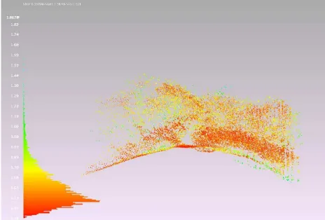
In this scene small walls, of less than 50cm in width and preserved to less than 1m in height are present among dense scrub, under a mixed deciduous canopy. In this case initial calculation of the roughness values at scales of 1, 3, 5, and 7 m reveal a different situation than at Montfaucon or Bregille. Here the lowest roughness values correspond predominantly to the understory canopy rather than to the terrain (figure 9).
Figure 9. Dominant vegetation in this scene results in the lowest roughness values at the 7m scale (shown here) appearing in the
understory canopy, and higher roughness values appearing on the terrain and standing archaeological remains. The results are the same at the 1,3, and 5m scales.
It is clear from this initial step that the approach taken at Montfaucon and Bregille will not succeed in this case, due to the extremely dense understory combined with the small scale of the features present. Rather than removing points with roughness values beyond 1σ in the roughness distribution, we invert the procedure and retain these points. The result is a point containing the majority of the terrain points and a number of vegetation components (figure 10).
Figure 10. The point cloud after the removal of points with roughness values within 1 σ in the point cloud.
The usual procedure is now followed, segmenting the cloud on roughness, local point density, and normal orientation. The resulting point cloud does not contain concentrations of low roughness returns with coherently oriented normals. Visits to the site reveal structures (figure 11) were not identified using the proposed approach. Based on a visual inspection of the point cloud we conclude that the small number of returns from these structures, fewer than 12 on a typical wall like the one in figure 10, prevents their successful identification using this approach.
Figure 11. Standing architecture on the scale of 40cm wide and 60cm tall, like the wall pictured here, is not successfully identified using the proposed approach.
4. RESULTS
In this paper three scenes were used to demonstrate an approach to the identification of standing architectural remains in mixed natural scenes using purely geometric measures of the point cloud. Using data collected at 8 pts/m2 standing architectural remains at the 2-3m scale (vertical height) are successfully
identified in medium density understory beneath a deciduous canopy. However, smaller remains, of less than 1m in height and located in dense understory canopy, are not detected. We predict that remains on this scale would be detected under similar vegetation conditions with ALS data collected at a higher point density.
We present two cases where the approach is successful in defining standing remains and one case, with under unfavourable vegetation conditions and where the scale of the features approaches the resolution of the data, where the approach is unsuccessful. We present both successful and unsuccessful cases here to illustrate both the potential and limitations of the proposed approach.
5. DISCUSSION
The principles of distinguishing standing archaeological remains, terrain and vegetation in ALS data by using local measures of roughness, density and normal orientation are established in this paper. The results presented here show that a combination of metrics results in a better classification than the use of a single multi-scale metric. For example, after the classification of the Bregille scene based on multi-scale roughness, some vegetation points are present in the segmented point cloud, which should only contain terrain and standing remains’ points. However, further segmentation on the basis of point density allows us to correctly identify these points as vegetation. Similarly, classification based solely on point densities (figure 12) confuses points from the terrain and denser vegetation components.
Figure 12. Local densities of the unsegmented point cloud at Chapel de Buis. Different components cannot be reliably segmented based solely on point density.
Terrain and standing architectural components of the point cloud have very similar roughness values across multiple scales, but can be clearly distinguished based on dominant normal direction because terrain components will have normals predominantly oriented towards the z-axis (except on extremely steep slopes) and standing architectural components will have normals predominantly oriented in the plane of the x-y axes. Even in the cases of relatively steep local slopes, as seen at Montfaucon (figure 4) the normals on the sloping terrain are oriented more strongly toward the z-axis than the normals from architectural components.
6. FUTURE WORK
The automation and optimization of this approach, so that it might be effectively applied to larger areas, is an obvious direction for future work. The automation of this approach would allow for the prospection of standing remains parallel to the prospection for microtopographic remains using ALS data currently widely practiced in archaeological research and cultural resource and heritage management.
Further testing of the approach using ALS data collected at higher and lower resolutions would be useful for establishing the limits of the approach in terms of the scale of the standing architectural remains which can be detected. Similarly, testing under other vegetation conditions would be useful in establishing the limits of this approach’s applicability.
References:
Axelsson, P. 2000. DEM generation from laser scanner data using adaptive TIN models. International Archives of Photogrammetry and Remote Sensing 33 (B4-1), pp.110-117.
Chen, C., Li, Y., Li, W., and Dai, H., 2013. A multiresolution hierarchical classification algorithm for filtering airborne LiDAR data. ISPRS Journal of Photogrammetry and Remote Sensing 82, pp. 1-9.
CloudCompare (version 2.4) [GPL software]. EDF R&D,
Telecom ParisTech (2013). Retrieved
from http://www.danielgm.net/cc/.
Dorninger, P. and Nothegger, C., 2007. 3D segmentation of unstructured point clouds for building modeling, in Stilla U et al (Eds) PIA07. International Archives of Photogrammetry, Remote Sensing and Spatial Information Sciences, 36 (3/W49A), pp. 191-196.
Doneus, M., Briese, C., Fera, M., and Janner, M., 2008. Archaeological Prospection of Forested Areas Using Full-waveform Airborne Laser Scanning. Journal of Archaeological Science 35 (4), pp. 882–893.
Ferraz, A., Bretar, F., Jacquemoud, S. Concalves, G. and Pereira, L., 2010. 3D segmentation of forest structure using an adaptive mean shift based procedure. Proceedings of SilviLaser 2010: The 10th International Conference on LiDAR Applications for Assessing Forest Ecosystems, pp. 280-290.
Forlani G., Nardinocchi C., Scaioni M., Zingaretti P., (2006): Complete classification of row LiDAR data and 3D reconstruction of buildings, Pattern Analysis and Applications 8, pp. 357–374.
Keller, W. and Borkowski, A., 2011. Wavelet based buildings segmentation in airborne laser scanning data set. Geodesy and Cartography 60 (2), pp. 99-121.
Lague, D. and Brodu, N., 2012. 3D terrestrial lidar data classification of complex natural scenes using a multi-scale dimensionality criterion: Applications in geomorphology. ISPRS Journal of Photogrammetry and Remote Sensing, 68, pp. 121-134.
Lague, D., Brodu, N. and Leroux, J. 2013. Accurate 3D comparison of complex topography with terrestrial laser scanner: Application to the Rangitikei canyon (N-Z). ISPRS Journal of Photogrammetry and Remote Sensing, 82, pp. 10-26.
Lalonde, J.-F., Vandapel, N., Huber, D.F., Hebert, M., 2006. Natural terrain classification using three-dimensional Ladar data for ground robot mobility. Journal of Field Robotics 23 (10), pp. 839–861.
Lasaponara, R., and Masini, N., 2009. Full-waveform Airborne Laser Scanning for the Detection of Medieval Archaeological Microtopographic Relief. Journal of Cultural Heritage 10 (Supplement 1), pp. 78–82.
MeshLab (version 1.32) [GPL software]. Visual Computing Lab - ISTI – CNR (2013) Retrieved from http://meshlab.sourceforge.net/.
Neidhart H., Sester M., (2008): Extraction of buildings ground planes from LiDAR data, International Archives of the Photogrammetry, Remote Sensing and Spatial Information Sciences, Vol. XXXVII, Part B2, pp. 405–410.
Opitz, R., 2009. Lidar Applications in Archaeology. Doctoral Thesis. University of Cambridge, Cambridge, pp. 289-341.
Opitz, R. and Cowley, D. (eds.), 2013. Interpreting Archaeological Topography – 3D Data, Visualization and Observation. Oxbow Books, Oxford.
Sim, K., Aung, Z. and Gopalkrishnan, V., 2010. Discovering Correlated Subspace Clusters in 3D Continuous-Valued Data. Proceedings of the ICDM 2010, pp. 471-480.
Vetter, M., et al., 2011. Vertical Vegetation Structure Analysis and Hydraulic Roughness determination using dense ALS point cloud data- a voxel based approach. International Archives of Photogrammetry, Remote Sensing and Spatial Information Sciences. Vol. XXXVIII(Part 5/W12), pp. 1-6 (digital media).
Wendt, H., Abry, P., Jaffard, S., 2007. Bootstrap for empirical multifractal analysis. IEEE Signal Processing Magazine 24 (4), pp. 38–48.
Acknowledgements
This research was carried out within the LIEPPEC Project, supported by the Region de Franche-Comte and the Observatoire des Dynamiques Industrielles et Territoriales (ODIT): Construction Historique des Espaces Forestiers (CHEF) program, generously supported by the EU Feder program. The authors gratefully acknowledge the support of both organizations.