isprsarchives XL 4 W2 95 2013

(1)

THE EXTENDED-OCTREE SPHEROID SUBDIVISION AND CODING MODEL

Xuefeng CAO*, Gang WAN, Feng LI, Ke LI,

Zhengzhou Institute of Surveying and Mapping, 450052 Zhengzhou, Henan, China - cxfchxy@163.com

KEY WORDS: extended-Octree model, global spatial grid, spheroid grid, grid subdivision, grid coding, spatial data model

ABSTRACT:

Discrete Global Grid has been widely used as the basic data model of digital earth. But it is only confined to the earth surface, and it can not reach to the earth inside or outside. The extended-Octree (e-Octree) spheroid subdivision and coding model proposed here provides a new kind of global 3D grid. This e-Octree model is based on the extension of octree structure, and there are three kinds of extended mechanisms including regular octree, degraded octree and adaptive octree. The process of partition and coding is discussed in details. The prototype system of e-Octree model is implemented, in which e-Octree model has been used to visualize global terrain and space object orbits. These typical applications experiments show that the e-Octree model could not only be used in global change research and earth system science, but also be used for dynamic simulation and spatial index.

* Corresponding author: Xuefeng CAO, cxfchxy@163.com. 1. INTRODUCTION

The range of human spatial activities have been promoted to various levels of space such as land, sea, air, sky, while spatial observation scope has been enlarged to every sphere shell of earth systems, and spatial exploration ability be enhanced. More and more scientific research and economic activities have shown itself such characteristics as global three-dimensional distribution, multi-spatial level, multi-temporal and spatial scale, cross specialties, so that these are depended on the construction of global uniform space framework and the integration of earth system information.

Discrete Global Grid gives a feasible way to meet this trend, and it has been widely used as the basic data model of digital earth (Goodchild, 2000). There have been a lot of researches on Discrete Global Grid data model, such as global data multi-hierarchical structure and indexing (Ottosm, 2002), global-scale image archiving model (Seong, 2005), and so on. The base of Discrete Global Grid model is grid subdivision. Usually, grid of GDG data model are mainly based on normal-polyhedron-based sphere partition, such as octahedron-based sphere grid (Dutton, 1999, Cui, 2009), dodecahedron-based sphere grid (Wickman, 1974), icosahedron-based sphere grid (Fekete, 1990). But it is only confined to the earth surface (Sahr, 2003), and it can not reach to the earth inside or outside. Therefore, the construction of global 3D grid becomes an important problem.

In recent years, several global 3D grid models have been proposed, such as Spheroid Latitude-Longitude Grid, Spheroid Yin-Yang Grid (Kageyama, 2004), Cubed-Sphere Grid (Tsuboi, 2008), Adaptive-Mesh Refinement Grid (Stadler, 2010), Sphere Degenerated Octree Grid (YU Jieqing, 2009). These 3D grid models are mainly used in earth system simulation, including geodynamo and mantle convection, global climate change, etc. But there are two problems. First, the partition method of the surface grid and the spheroid grid is dissevered. Global surface grid focus on the spatial data of earth surface, whereas the data inside and outside of earth is ignored. In Global 3D grid models, the earth is considered as a sphere, and the partition is took place in the 3D space. Then it is naturally to organize 3D data. But the surface data, such as remote sensing images, elevation data, could not be processed favourably. Second, the sphere shell 3D structure, which is the basic spatial character of earth

system, has not been reflected distinctly. In fact, the spatial information granularity and the modelling and representation requirement of different level of space are different.

This paper is to present a subdivision and coding model of global 3D grid, called as extended-Octree (e-Octree) model. In the e-Octree model, global 3D space is partitioned into several sphere shells, and then the sphere shell 3D space is subdivided recursively. There are three kinds of recursive subdivision mechanisms: regular octree, degraded octree and adaptive octree. These three mechanisms bring great agility and adjustability. The e-Octree model can be served as a global spatial grid framework for global spatial data organization and representation.

2. THE E-OCTREE SUBDIVISION

In the e-Octree model, global 3D space of earth system is considered as several homocentric sphere shells. The e-Octree subdivision process consists of two main steps: the partition of sphere shells and the subdivision of sphere shell volume.

2.1 The Partition of Sphere Shells.

Sphere shell is the basic notion in this paper. It is different from earth system sphere, such as hydrosphere, biosphere and lithosphere. Sphere shell is the mathematic abstraction of earth spheres, which is defined in mathematic formula. It consists of the inside sphere shell surface, the outside sphere shell surface and the sphere shell volume.

The sphere shell surface is one sphere with a radius. The radius of inside sphere shell surface is r, and r+Δr for the

outside sphere shell surface. Δr is the thickness of the sphere

shell.

The sphere shell volume is the 3D space between inside and outside sphere shell surface, its radial thickness is Δr.

2.2 The Subdivision of Sphere Shell Volume

The second step is the subdivision of sphere shell volume. But this step is taken place both at sphere shell surface and sphere shell radius, which is discussed as below.

International Archives of the Photogrammetry, Remote Sensing and Spatial Information Sciences, Volume XL-4/W2, 2013 ISPRS WebMGS 2013 & DMGIS 2013, 11 – 12 November 2013, Xuzhou, Jiangsu, China

(2)

The subdivision of sphere shell surface is based on partition curve. First, the sphere shell surface is considered as a normal sphere, it is divided into six approximately equal area faces, four faces along low latitude and two faces near north and south polar, the boundary (yellow line in Finger 1) is latitude 45°. This level is noted as level 0.

Figure 1. Six equal area faces

Second, the partition curve is constructed for each face. In Finger 2 and 3, the red lines are called b-curve, the green line is called l-curve. The subdivision result of face 0 is shown in Finger 2.

(a) level 1 (b) level 2 (c) level 3 Figure 2. Sphere shell surface subdivision of face 0 After the first level subdivision of face 4, there are 4 subcells, one of them is shown in Finger 2(a). The next two level subdivision result of face 4 is shown in Finger 2 (b) and (c).

(a) level 2 (b) level 3 (c) level 3 Figure 3. Sphere shell surface subdivision of face 4 The benefits of the sphere shell surface subdivision are that all of global grid cells are organized using quadtree structure, and grid cells with low latitude are regular geographic quad while there is no singularity at North Pole or South Pole. In fact, the length of each edge of these six faces is the same 90°, which is the important advantage for grid cell calculation.

The partition curves (b-curve and l-curve) are extended from sphere surface to spheroid 3D space. In Finger 4 and 5, the gray fan is the partition curve surfaces. These two kinds of partition curve surfaces are used to carve the solid space into subvolumes.

(a) low latitude (b) high latitude

Figure 4. The partition curve surface corresponding to l-curve

(a) low latitude (b) high latitude

Figure 5. The partition curve surface corresponding to b-curve The subdivision of sphere shell radial is directly halving the thickness recursively.

2.3 The recursive subdivision of sphere shell volume cell

Until now, global 3D space is divided into several sphere shells, and each sphere shell is divided into six basic sphere shell volume cells (Finger 6).

(a)inner sphere shell (b)outer sphere shells Figure 6. The basic cells of sphere shell volume. The following operation is the recursive subdivision of each sphere shell volume cell.

There are three kinds of subdivision : regular octree subdivision (ROS), degraded octree subdivision (DOS) and adaptive octree subdivision (AOS).

2.3.1 Regular Octree Subdivision: The basic structure of 3D grid is octree. According to the regular octree structure, one grid cell is subdivided into eight subcells. The regular octree subdivision is took place both at surface and radial. The subdivision of first three subdivision levels is shown in Finger 7 and 8.

(a) level = 0 (b) level = 1 (c) level = 2 Figure 7. ROS near equator

(a) level = 0 (b) level = 1 (c) level = 2 Figure 8. ROS near north polar

0 1 2 3

4

5

(3)

2.3.2 Degraded Octree Subdivision: It is obvious that these subcells of ROS are large differences in volume. One feasible way to mitigate the effect is degradation. These four inner subcells are combined into one subcell. The DOS results are shown in Figure 9 and 10. It is noteworthy that outside subdivision is denser than inside.

(a) level = 0 (b) level = 1 (c) level = 2 Figure 9. DOS near equator

(a) level = 0 (b) level = 1 (c) level = 2 Figure 10. DOS near north polar

2.3.3 Adaptive Octree Subdivision: In fact, the subdivision on surface or radial could be executed several times first, and then the subdivision operation takes place synchronously. In Figure 11, the subdivision is performed on surface independently, while Figure 12 on radial.

(a) level = 0 (b) level = 1 (c) level = 2 Figure 11. AOS near equator

第0级第1级第2级

Figure 12. AOS near north polar

3. THE E-OCTREE CODING

The basic idea of grid code format of e-Octree is = (l, k, j, i), as shown in Figure 13. l denotes the subdivided level, k, j, i denotes the number on each dimensional.

Figure 13. The e-Octree coding structure

Such a basic code (l, k, j, i) could be directly used for ROS. It should be added some parameters for DOS and AOS. For DOS,

it should include the degradation flag. For AOS, it should include the independent subdivision level.

The e-Octree grid code formalization format is

SolidCellCode = { DatumSphereTag, SolidSubdivideTag }.

In this format,

DatumSphereTag = { DatumSphereID | DatumSphereID ∈ Z }.

SolidSubdivideTag = { ( RootSolidID, Level, RadialSegID, SphericalRowID, SphericalColID ) | RootSolidID, Level,

RadialSegID, SphericalRowID, SphericalColID ∈ N }.

DatumSphereTag denotes the tag of datum sphere,

DatumSphereID denotes the number of datum sphere, SolidSubdivideTag denotes the subdivision method, RootSolidID denotes the root cell, Level denotes the sundivision

level, RadialSegID denotes the number of radial cell segment,

SphericalRowID denotes the row number of grid cell on the

sphere shell surface, SphericalColID denotes the column number of grid cell on the sphere shell surface.

3.1 ROS Code

According to the above format, the format of ROS grid cell is：

SolidCellCode = ( DatumSphereID, RootSolidID, Level, RadialSegID, SphericalRowID, SphericalColID ).

Then the transformation between SolidCellCode and (lat, lon, r) is discussed as below.

Two assumptions are given:

• The inner sphere shell surface of the datum sphere volume with number DatumSphereID is noted as R (R ≥ 0), its thickness is noted as ΔR (ΔR > 0), so that the radius of the

outer sphere shell surface is R+ΔR .

• The radial span of the grid cell with the Level subdivision is noted as SpanLevel.

3.1.1 ROS Coding

The geographic coordinate of one point (lat, lon) and datum sphere shells’ parameters are all given, then calculate the grid cell code at Level.

First, ransack these datum sphere shells in order to confirm the datum sphere number which this point falls in.

for each DatumSphere with id if R ≤ r < R+ΔR

DatumSphereID = id

Second, calculate the corresponding radial cell code:

RadialSegID = 2Level × ( r – R ) / ΔR .

Third, calculate the corresponding surface grid cell code. Introduce temporary variables x, y:

x = ( lat + 90° ) / 180°,

y = ( lon + 180° ) / 360°. Confirm the RootSolidID:

if -45°≤ lat < 45°

RootSolidID = floor ( 4 × y )

else if lat ≥ 45°

RootSolidID = 4

else

RootSolidID = 5

Introduce temporary variables a, x’, y’:

a = floor ( 4 × y ),

if a == 4 a = 3,

x' = 4 × y – a, y’ = 2 × x – 0.5.

Introduce temporary variable t, and calculate SphericalRowID and SphericalColID:

if RootSolidID < 4

SphericalRowID = floor ( y’ × 2Level₎ J

I i

j

O K

(4)

SphericalColID = RootSolidID × 2Level_{+ floor ( x’ × 2}Level₎

The grid cell code is given, then calculate the coordinate of the leftbottom corner point (lat, lon, r).

First, calculate the radial span of the grid cell with the Level subdivision and r:

SpanLevel = Δ R / 2Level,

r = R + RadialSegID × SpanLevel . Then we get:

RootSolidID = SphericalColID / 2Level, Second, introduce temporary variables x, y, t, x’,

x = ( SphericalColID –RootSolidID × 2Level ) / 2Level ,

y = SphericalRowID / 2Level,

t = 0, x’ = x.

Then calculate the geographic coordinate of this corner point (lat, lon):

The format of DOS grid cell is：

DegeneratedSolidCellCode = ( DatumSphereID, RootSolidID, Level, RadialSegID, InnerCombinateSign, SphericalRowID, SphericalColID ).

Then the transformation between DegeneratedSolidCellCode and (lat, lon, r) is discussed as below.

These assumptions are same to ROS Code.

3.2.1 DOS Coding

The geographic coordinate of one point (lat, lon) and datum sphere shells’ parameters are all given, then calculate the grid cell code at Level.

First, the datum sphere number which this point falls in is confirmed by ransack these datum sphere shells.

RadialSegID = 2Level × ( r – R ) / ΔR

if RadialSegID mod 2 == 0

InnerCombinateSign = true

else

InnerCombinateSign = false

Third, calculate the corresponding surface grid cell code. These temporary variables x, y are same to ROS Coding, and also the confirmation of RootSolidID:

After the calculation of SphericalRowID and SphericalColID using ROS Coding, the transformation is different as shown below:

if InnerCombinateSign == true

SphericalRowID = floor ( y’ × 2Level - 1 )

SphericalColID = RootSolidID × 2Level - 1 + floor ( x’ × 2Level - 1 ) else

SphericalRowID = floor ( y’ × 2Level )

SphericalColID = RootSolidID × 2Level + floor ( x’ × 2Level )

3.2.2 DOS Decoding

The decoding calculation is almost same to ROS decoding except for the calculation of the radial span of the grid cell with the Level subdivision and r:

SpanLevel = Δ R / 2Level,

r = R + RadialSegID × SpanLevel , if InnerCombinateSign = = true, Level = Level – 1.

3.3 AOS Code

The format of AOS grid cell is：

AdaptiveRegularSolidCellCode = ( DatumSphereID, InitRadialLevel, InitSphericalLevel, RootSolidID, Level, RadialSegID, SphericalRowID, SphericalColID ).

Then the transformation between this grid code and (lat, lon, r) is discussed as below.

These assumptions are same to ROS Code.

3.3.1 AOS Coding

First, the confirmation of the datum sphere number is same to ROS Coding.

RadialSegID = 2Level + InitRadialLevel × ( r – R ) / ΔR.

Third, calculate the corresponding surface grid cell code using the same method of ROS Coding.

(5)

After the calculation of SphericalRowID and SphericalColID using ROS Coding, the transformation is different as shown below:

SphericalRowID = floor ( y’ × 2Level+ InitRadialLevel)

SphericalColID = RootSolidID × 2Level

+ floor ( x’ × 2Level+InitRadialLevel )

3.3.2 AOS Decoding

First, calculate the radial span of the grid cell with the Level subdivision and r:

SpanLevel = Δ R / 2Level+ InitRadialLevel,

r = R + RadialSegID × SpanLevel . Then we get:

RootSolidID = SphericalColID / 2Level + InitRadialLevel

Second, introduce temporary variables x, y, t, x’,

x = ( SphericalColID –RootSolidID × 2Level+ InitRadialLevel )

/ 2Level+ InitRadialLevel ,

y = SphericalRowID / 2Level,

t = 0, x’ = x.

Then calculate the geographic coordinate of this corner point (lat, lon) using the same process of ROS Decoding.

4. THE E-OCTREE PROTOTYPE

The prototype system of e-Octree model is implemented. Global terrain, space object orbits and movement visualization are chose as typical applications. These experiments are tested on one notebook PC with CPU Core2 Duo 2.0GHz, memory 2GB, Geforce 8600M GT, 1280

×

800 display resolution. The first experiment is global terrain visualization. The e-Octree model is used to organize elevation, images and maps. Testing data includes SRTM elevation (30 seconds resolution, 3.56GB), BlueMarble Image (30 seconds resolution, 3.6GB) and vector map (1:4,000,000, National Borderline 1.1MB, Province Borderline 1.7MB, Roadway and Railway 17MB). The total amount of data is nearly 8GB. And the rendering efficiency is stably near 45 fps.

Figure 14. The e-Octree model grid and global terrain

Figure 15. The e-Octree model grid and regional terrain

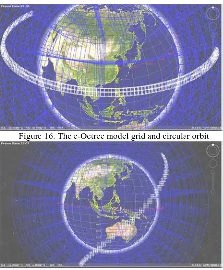
Figure 16. The e-Octree model grid and circular orbit

Figure 17. The e-Octree model grid and arbitrary orbit In the second experiments, the e-Octree model is used to represent the orbit of different satellites and the position change during movement. These grid frame cells, position code are all generated real time. The rendering efficiency is stably near 40 fps during the whole test.

Figure 18. The e-Octree model grid and satellite’s position 1

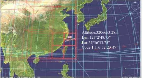
Altitude:3206653.28m

Lon:121°38′26.25″

Lat:24°36′33.75″

Code:1-1-6-32-22-49 Altitude:3206653.28m

Lon:120°14′3.75″

Lat:4°36′33.75″

Code:1-1-6-32-21-49

(6)

5. CONCLUSIONS

A new global 3D grid is proposed in this paper, called extended-Octree (e-Octree) spheroid subdivision and coding model. The e-Octree model includes three kinds of subdivision mechanisms: regular octree subdivision, degraded octree subdivision and adaptive octree subdivision. The partition and coding process is given out in details. The e-Octree model prototype is implemented, and global terrain and space object orbits visualization are chose as typical experiments. These results show that the e-Octree model could not only be used in global change research and earth system science, but also be used for dynamic simulation and spatial index.

REFERENCES

Cui Majun, Zhao Xuesheng. (2007) Tessellation and distortion analysis based on spherical DQG. Geography and Geo-Information Science, 23(6), pp.23~25.

Dutton, G. (1999) A hierarchical coordinate system for geoprocessing and cartography. Springer-Verlag . Berlin, Germany.

Fekete, G. (1990) Rendering and managing spherical data with sphere quadtrees. Proceedings of the Visualization’90 IEEE Computer Society, pp.176-186.

Goodchild M. (2000) Discrete global grids for digital earth. In: International Conference on Discrete Global Grids, California: Santa Barbara.

Kageyama A, Tetsuya Sato. (2004) The Yin-Yang Grid : An Overset Grid in Spherical Geometry. Geochenmistry Geophisics Geosystems, 5(9) , pp.1-15．

Ottosm, Hauska. (2002) Ellipsoidal quadtree for indexing of global geographical data. International Journal of Geographical Information Science, 16(3), pp.213-226.

Sahr K, White D, Kimerling A. (2003) Geodesic Discrete Global Grid Sytems．Cartography and Geographic Information Science, 30(2), pp.121-134．

Seong, J. C. (2005) Implementation of an equal-area girding method for global-scale image archiving. Photogrammetric Engineering & Remote Sensing, 71(5), pp.623-627.

Stadler G, Gurnis M, Burstedde C. (2010) The Dynamics of Plate Tectonics and Mantle Flow: From Local to Global Scales. Science, 329(5995) , pp.1033-1038.

Tsuboi S, Komatitsch D. JI C. (2008) Computations of global sisimic wave propageation in three dimensional Earth mode. High Performance Computing. pp. 434-443.

Wickman, F. E., Elvers, E., Edvarson, K. (1974) A system of domains for global sampling problems. Geografiska Annaler, 56(3/4), pp.201~212.

YU Jieqing, WU Lixin. (2009) Spatial subdivision and coding of a global three-dimensional grid: spheroid degenerated-octree

grid. International geoscience & remote sensing symposium, Capetown, Africa.

ACKNOWLEDGEMENTS

This publication is based on work supported by the National Natural Science Foundation of China (Grant No. 41371384).

Altitude:3206653.28m

Lon:123°2′48.75″

Lat:24°36′33.75″

Code:1-1-6-32-23-49