Grassland modeling and monitoring with SPOT-4 VEGETATION
instrument during the 1997–1999 SALSA experiment
P. Cayrol
a,∗, A. Chehbouni
b, L. Kergoat
c, G. Dedieu
a, P. Mordelet
a, Y. Nouvellon
daCESBIO (CNRS/CNES/UPS), 18 av. E. Belin, bpi 2801, 31401 Toulouse Cedex 4, France bIRD/IMADES, Col. San Benito, 83190 Hermosillo, Sonora, Mexico
cLET (CNRS/UPS), 13 av. col. Roche, BP 4403, 31405 Toulouse Cedex, France dUSDA-ARS, 2000 E. Allen Road, Tucson, AZ 85719, USA
Abstract
A coupled vegetation growth and soil–vegetation–atmosphere transfer (SVAT) model is used in conjunction with data collected in the course of the SALSA program during the 1997–1999 growing seasons in Mexico. The objective is to provide insights on the interactions between grassland dynamics and water and energy budgets. These three years exhibit drastically different precipitation regimes and thus different vegetation growth.
The result of the coupled model showed that for the 3 years, the observed seasonal variation of plant biomass, leaf area index (LAI) are well reproduced by the model. It is also shown that the model simulations of soil moisture, radiative surface temperature and surface fluxes compared fairly well with the observations.
Reflectance data in the red, near infrared, and short wave infrared (SWIR, 1600 nm) bands measured by the VEGETATION sensor onboard SPOT-4 were corrected from atmospheric and directional effects and compared to the observed biomass and LAI during the 1998–1999 seasons. The results of this ‘ground to satellite’ approach established that the biomass and LAI are linearly related to the satellite reflectances (RED and SWIR), and to vegetation indices (NDVI and SWVI, which is a SWIR-based NDVI). The SWIR and SWVI sensitivity to the amount of plant tissues were similar to the classical RED and NDVI sensitivity, for LAI ranging from 0 and 0.8 m2m−2and biomass ranging from 0 to 120 g DM m−2.
Finally, LAI values simulated by the vegetation model were fed into a canopy radiative transfer scheme (a ‘model to satellite’ approach). Using two leaf optical properties datasets, the computed RED, NIR and SWIR reflectances and vegetation indices (NDVI and SWVI) compared reasonably well with the VEGETATION observations in 1998 and 1999, except for the NIR band and during the senescence period, when the leaf optical properties present a larger uncertainty. We conclude that a physically-sound linkage between the vegetation model and the satellite can be used for red to short wave infrared domain over these grasslands. These different results represent an important step toward using new generation satellite data to control and validate model’s simulations at regional scale. © 2000 Published by Elsevier Science B.V.
Keywords:SVAT; Grassland; Semi-arid; VEGETATION; SWIR; SALSA
1. Introduction
Both natural (floods, fires, droughts, volcanoes, etc.) and human (deforestation, overgrazing, urbanization
∗Corresponding author. Tel.:+33-5-61-55-85-24;
fax:+33-5-61-55-85-00.
E-mail address:[email protected] (P. Cayrol).
and pollution) influences are known to cause massive changes in vegetation cover and dynamics. Drastic changes in land surface properties, such as those oc-curring because of deforestation or the desertification processes are likely to have climatic consequences. There is increasing evidence pointing towards the im-portant role played by land-atmosphere interactions
in controlling regional, continental and global cli-mate. The fluxes of energy, mass and momentum from the land-surface adjust to and alter the state of the atmosphere in contact with land, allowing the po-tential for feedback at several time and spatial scales. A better understanding of land atmosphere feedback could thus provide answers to questions regarding the climatic implications of land use/cover change, land surface heterogeneity, and of atmospheric com-position. Model simulations (Bonan et al. (1992), and Nobre et al. (1991) among others) have shown that drastic changes in vegetation type and cover cause significant impacts on simulated continental-scale cli-mate. Avissar (1995) reviews examples of model and observational evidence showing that regional-scale precipitation patterns are affected by land surface features such as discontinuities in vegetation type. In addition, fluxes of CO2 and other greenhouse gases also depend on the biophysical properties of the land surface. Changes in land cover, land use and climate modify the uptake and release of these gases, lead-ing to changes in their atmospheric concentrations which in turn may influence the global atmospheric circulation.
Plant canopy regulates the exchanges of mass, en-ergy and momentum in the biosphere–atmosphere interface. It dominates the functioning of hydrolog-ical processes through modification of interception, infiltration, surface runoff, and its effects on surface albedo, roughness, evapotranspiration, and root sys-tem affect soil properties. The amount of vegetation controls the partitioning of incoming solar energy into sensible and latent heat fluxes, and consequently changes in vegetation levels will result in long-term changes in both local and global climates and in turn will affect the vegetation growth as a feedback. In marginal ecosystems, such as arid and semi-arid areas, this may result in persistent drought and de-sertification, with substantial impacts on the human populations of these regions through reduction in agri-cultural productivity, reduction in quantity and quality of water supply, and removal of land from human habitability. It is, therefore, scientifically and socially important to study arid ecosystems so that the impact of management practices on the scarce resources can be understood. In this regard, a better understanding of soil–vegetation–atmosphere exchange processes at different time–space scale must be achieved in order
to document the complex interactions between the atmosphere and the biosphere.
During the last decades, vegetation models have been designed to simulate the seasonal and inter-annual variability in plant structure and function. To provide insights on the interaction between terrestrial ecosystems and the atmosphere, some of these vegeta-tion models are now being coupled to soil–vegetavegeta-tion– atmosphere transfer-scheme (SVATs) (e.g. Lo Seen et al., 1997; Calvet et al., 1998a) and even interact with atmospheric models (e.g. to meso-scale model, Pielke et al., 1997; or to GCM, Dickinson et al., 1998). However, the development of process-based models is accompanied by increasing difficulties in obtaining values for the numerous parameters requi-red by the models. This has been pointed out by Gupta et al. (1998) in the case of hydrological models. The vegetation models are also confronted by this tion problem (e.g. Calvet et al., 1998b). The calibra-tion of these models proves especially difficult and time-consuming when regional and long-term simu-lations are to be carried out.
In this study, a coupled vegetation growth and SVAT model (V–S model) developed and validated using Hapex–Sahel data (Cayrol et al., in press) has been used to simulate surface radiation, turbulent heat and mass, liquid water and the control of water vapor and CO2fluxes. Data collected during the semi-arid land– surface–atmosphere (SALSA) program (Goodrich et al., 2000) over grassland site in Mexico during three growing seasons (1997–1999) have been used to assess the performance of the model.
The specific questions addressed in the paper are: 1. Can this coupled model initially developed for the
Sahel environment be used in Mexico, and what level of adaptation/calibration is required? 2. Can this model capture the consequences of the
ob-served inter-annual variability of the precipitation in terms of surface fluxes and vegetation develop-ment?
3. Is it possible to monitor the surface biophysical parameters using NDVI and/or SWVI as surrogate measures, the ‘ground-to-satellite’ approach? 4. Can the vegetation growth/SVAT model, when
This paper is organized as follows. Section 2 describes both the ground and satellite data sets collected during 1997–1999 seasons. Section 3 presents a brief descrip-tion of the model and calibradescrip-tion procedure. Secdescrip-tion 4 presents an assessment of the performance and ro-bustness of the model. In Section 5, measurements ac-quired by the new VEGETATION sensor in 1998 and 1999 are also related to biophysical parameters such as green biomass and leaf area index (LAI). Finally, we present a comparison between predicted and observed radiative variables (i.e. reflectances) using VEGETA-TION sensor. The V–S model was coupled with a radiative transfer model in order to assess its capabil-ity to simulate the seasonal variation of visible, near infrared and short wave infrared surface reflectances.
2. Site and data description
The study site is located in the upper San Pedro basin (near Zapata village, 110◦09′W; 31◦01′N; el-evation 1460 m) and was the focus of the SALSA activities in Mexico during the 1997–1999 field cam-paigns. The natural vegetation is composed mainly of perennial grasses of which the dominant genus is Bouteloua, and the soil is mainly sandy loam (67% of sand and 12% of clay).
2.1. Field data
A 7 m tower has been erected in the beginning of 1997 season and equipped with instruments to measure conventional meteorological data (incoming radiation and net radiation at a height of 1.7 m with REBS Q6 net radiometer). The soil heat flux was estimated us-ing six HFT3 plates from REBS Inc., WA, USA. Wind speed and direction, precipitation, air temperature and humidity were also measured. Soil moisture was measured using Time Domain Reflectometry (TDR) sensors (Campbell Scientific CS615 reflectometer) at two locations and four different depths (5, 10, 20 and 30 cm) and a capacity probe (ThetaProbe) which gives an integrated measurement of the water content over the first 5 cm of the soil layer. Radiative surface temperature was measured using Everest Interscience infrared radiometers (IRT) with a 15◦field of view at two different viewing angles (0 and 45◦). The band pass of these radiometers is nominally 8–14mm.
Sensible and latent heat fluxes were determined using from the Eddy covariance method. The system is made up of a three-axis sonic anemometer manu-factured by Gill Instrument (Solent A1012R) and an IR gas analyzer (LI-COR 6262 model) which is used in a close path mode. The system is controlled by a specially written software, which calculates the sur-face fluxes of momentum, sensible and latent heat and carbon dioxide. However, during a large part of the ex-periment, some problems with the LICOR instrumen-tation did not permit the derivation of latent heat and CO2 fluxes. Therefore, latent heat flux was derived from measurements of sensible heat flux and avail-able energy at the surface as the residual term of the surface energy budget. In 1998, an additional Bowen ratio system has been installed in the same site for a 3 weeks period. Note that the main source of uncertainty concerns the surface soil heat flux. Kustas et al. (1999) showed that uncertainty in soil heat flux is probably larger that the 30% reported in Stannard et al. (1994). Braud et al. (1993) also pointed out the problem as-sociated with the estimation of latent heat flux as the residual term of the energy balance equation given the uncertainty in available energy measurements.
The evolution of the biomass was monitored dur-ing the 1997–1999 growdur-ing seasons from day of year (DoY) 182–285. The adopted protocol was to cut 10 samples of 1 m2 of biomass along a 100 m tran-sect. Then live phytomass and standing necromass were separated and weighted and the samples were weighted again after 48 h drying at 70◦C.
The LAI was determined from biomass and specific leaf area (SLA) measurements (Nouvellon, 1999). In 1998, grass stomatal resistance was measured using two automatic porometers (models MK3 and AP4, Delta T Devices, Ltd, Cambridge, UK).
2.2. Satellite data
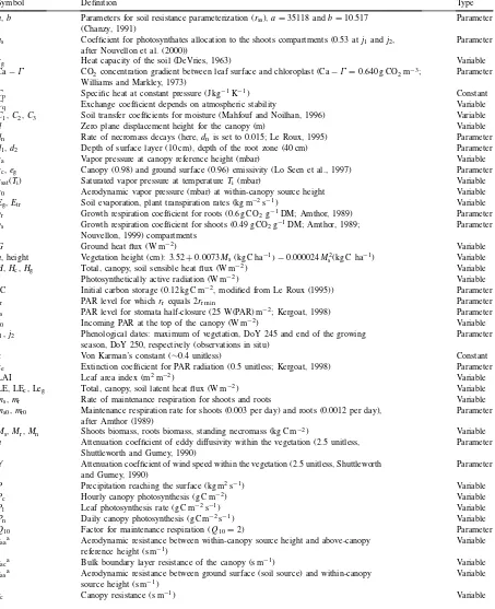
Table 1
Listing of the variables, parameters and constants used in the vegetation-SVAT model
Symbol Definition Type
a,b Parameters for soil resistance parameterization (rss),a=35118 andb=10.517 (Chanzy, 1991)
Parameter
as Coefficient for photosynthates allocation to the shoots compartments (0.53 atj1andj2, after Nouvellon et al. (2000))
Parameter
cg Heat capacity of the soil (DeVries, 1963) Variable
Ca−Γ CO2concentration gradient between leaf surface and chloroplast (Ca−Γ =0.640 g CO2m−3; Williams and Markley, 1973)
Parameter
Cp Specific heat at constant pressure (J kg−1K−1) Constant
Cq Exchange coefficient depends on atmospheric stability Variable
C1,C2,C3 Soil transfer coefficients for moisture (Mahfouf and Noilhan, 1996) Variable
d Zero plane displacement height for the canopy (m) Variable
dn Rate of necromass decays (here,dn is set to 0.015; Le Roux, 1995) Parameter
d1,d2 Depth of surface layer (10 cm), depth of the root zone (40 cm) Parameter
ea Vapor pressure at canopy reference height (mbar) Variable
ec,eg Canopy (0.98) and ground surface (0.96) emissivity (Lo Seen et al., 1997) Parameter
esat(Ti) Saturated vapor pressure at temperatureTi (mbar) Variable
e0 Aerodynamic vapor pressure (mbar) at within-canopy source height Variable
Eg,Etr Soil evaporation, plant transpiration rates (kg m−2s−1) Variable
gr Growth respiration coefficient for roots (0.6 g CO2 g−1DM; Amthor, 1989) Parameter
gs Growth respiration coefficient for shoots (0.49 g CO2g−1DM; Amthor, 1989; Nouvellon, 1999) compartments
Parameter
G Ground heat flux (W m−2) Variable
h, height Vegetation height (cm): 3.52+0.0073Ms (kg C ha−1)−0.000024Ms2(kg C ha−1) Variable
H,Hc,Hg Total, canopy, soil sensible heat flux (W m−2) Variable
I Photosynthetically active radiation (W m−2) Variable
IC Initial carbon storage (0.12 kg C m−2, modified from Le Roux (1995)) Parameter
Ir PAR level for whichrrequals 2rr min Parameter
Is PAR level for stomata half-closure (25 W(PAR) m−2; Kergoat, 1998) Parameter
I0 Incoming PAR at the top of the canopy (W m−2) Variable
j1,j2 Phenological dates: maximum of vegetation, DoY 245 and end of the growing season, DoY 250, respectively (observations in situ)
Parameter
k Von Karman’s constant (∼0.4 unitless) Constant
ke Extinction coefficient for PAR radiation (0.5 unitless; Kergoat, 1998) Parameter
LAI Leaf area index (m2m−2) Variable
LE, LEc, Leg Total, canopy, soil latent heat flux (W m−2) Variable
ms,mr Rate of maintenance respiration for shoots and roots Variable
ms0,mr0 Maintenance respiration rate for shoots (0.003 per day) and roots (0.0012 per day), after Amthor (1989)
Parameter
Ms,Mr,Mn Shoots biomass, roots biomass, standing necromass (kg C m−2) Variable
n Attenuation coefficient of eddy diffusivity within the vegetation (2.5 unitless, Shuttleworth and Gurney, 1990)
Parameter
n′ Attenuation coefficient of wind speed within the vegetation (2.5 unitless, Shuttleworth
and Gurney, 1990)
Parameter
P Precipitation reaching the surface (kg m2s−1) Variable
Pc Hourly canopy photosynthesis (g C m−2) Variable
Pl Leaf photosynthesis rate (g C m−2s−1) Variable
Pn Daily canopy photosynthesis (g Cm−2s−1) Variable
Q10 Factor for maintenance respiration (Q10=2) Parameter
raaa Aerodynamic resistance between within-canopy source height and above-canopy reference height (s m−1)
Variable
raca Bulk boundary layer resistance of the canopy (s m−1) Variable
rasa Aerodynamic resistance between ground surface (soil source) and within-canopy source height (s m−1)
Variable
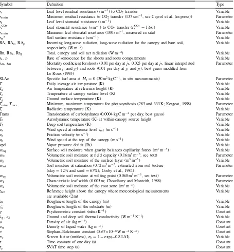
Table 1 (Continued)
Symbol Definition Type
rr Leaf level residual resistance (s m−1) to CO2transfer Variable
rr min Minimum residual resistance to CO2transfer (137 s m−1, see Cayrol et al. (in press)) Parameter
rs Leaf level stomatal resistance (s m−1) Variable
rCO2
s Leaf stomatal resistance (s m−1) to CO2 transfer (rsCO2=1.6rs) Variable
rs min Minimum leaf stomatal resistance (100 s m−1, measured in situ) Parameter
rssa Soil surface resistance (s m−1) Variable
RA, RAc, RAg Incoming long-wave radiation, long-wave radiation for the canopy and bare soil, respectively (W m−2)
Variable
Rn, Rnc, Rng Total, canopy and soil net radiation (W m−2) Variable
ss,sr Rate of senescence for the shoots and roots compartments Variable
ss0,sr0 Mortality coefficient for shoots (0.01 per day atj1, 0.025 per day atj2, linear interpolated betweenj1andj2) and roots (0.01 per day atj1andj2), best guess modified from Le Roux (1995)
Parameter
SLAo Specific leaf area atMs=0 (30 m2kg C−1, in situ measurements) Parameter
T Daily average air temperature (K) Variable
Ta Air temperature at reference height (K) Variable
Tc Temperature at canopy surface level (K) Variable
Tg Ground surface temperature (K) Variable
Tmin,Tmax Minimum, maximum temperature for photosynthesis (283 and 333 K; Kergoat, 1998) Parameter
Tr Radiative temperature (K) Variable
Trans Translocation of carbohydrates (0.0004 kg C m−2 per day, best guess) Parameter
T0 Aerodynamic temperature (K) at within-canopy source height Variable
T2 Deep soil temperature (K) Variable
ua Wind speed at reference levelzref (m s−1) Variable
ua Friction velocity (m s−1) Variable
uh Wind speed at the top of the canopy (m s−1) Variable
vpd Vapor pressure deficit (Pa) Variable
weq Surface soil moisture when gravity balances capillarity forces (m3m−3) Variable
wfc Volumetric soil moisture at field capacity (0.16 m3m−3, see text) Parameter
wg Volumetric soil moisture of the surface layer (m3m−3) Variable
wsat Soil moisture at saturation (0.42 m3m−3, estimated from soil texture (clay=12% and sand=67%); Cosby et al., 1984)
Parameter
wwp Volumetric soil moisture at wilting point (0.068 m3m−3, see text) Parameter
w1 Characteristic leaf width (0.005 m; Choudhury and Monteith, 1988) Parameter
w2 Volumetric soil moisture of the root zone (m3m−3) Variable
zref Reference height above the canopy where meteorological measurements are available (2 m)
Variable
z0 Roughness length of the canopy (m) Variable
z′
0 Roughness length of the substrate (m) Variable
γ Psychrometric constant (mbar K−1) Constant
λg,λ2 Ground and deep soil thermal conductivity (W m−1K−1) Variable
ρ Density of air (kg m−3) Constant
ρw Density of liquid water (kg m−3) Constant
σ Stephan–Bolztmann constant (5.67×10⁻⁸W m−2K−4) Constant
σf Screen factor (unitless),σf=1−exp(−0.8 LAI) Variable
τ Time constant of one day (s) Constant
τp SVAT time step (s) Constant
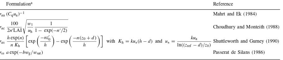
aResistances formulations can be found in Table 2. LST by the VEGETATION instrument onboard SPOT-4 (http://sirius-ci.cst.cnes.fr:8080/). VEGETATION is a large field-of-view instrument providing measure-ments in four spectral bands, namely: blue (0.43–0.47
We used VEGETATION P-products, which consist of top of the atmosphere reflectance, geometrically corrected and remapped with a multi-temporal and absolute accuracy better than 1 km. A VEGETATION dedicated version of SMAC (Berthelot and Dedieu, unpublished) was used for atmospheric corrections. Water vapor fields at 1×1◦resolution were derived from atmospheric analyses of the French weather forecast operational model available every 6 h. This procedure for atmospheric correction is now used for the operational processing of VEGETATION data.
VEGETATION and AVHRR sensors have a large field of view, which implies large view zenith angle variations from roughly 0 to±65◦. The reflectances can vary by factors of two or three, depending on the sun-sensor geometry. This implies that these direc-tional effects have to be corrected. One of the options to minimize these effects is through the use of the so-called vegetation indices. Two vegetation indices were calculated: NDVI=(NIR−RED/(NIR+RED) and SWVI=(NIR−SWIR)/(NIR+SWIR). Normal-ized reflectance were also computed to remove the ef-fect of surface anisotropy on the VEGETATION data, as described in Appendix A.
3. Model description and calibration procedure
3.1. Model description
An extensive description of the Vegetation-SVAT model (V–S model) which is used in this study can be found in Cayrol et al. (in press). The mains equations solved by the model are summarized in the Appendix B. Schematically, the vegetation growth model pro-vides the LAI, which is then used by the SVAT in the
Table 2
aAll the symbols are defined in Table 1.
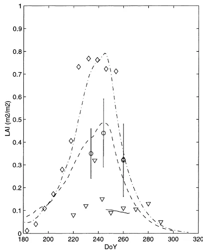
Fig. 1. Observed (▽,sande) and simulated (–, – – and –·) sea-sonal evolution of the aboveground biomass for years 1997–1999, respectively. Error bars indicate the standard deviation.
computation of the energy partitioning between soil and the vegetation as well as in the parameterization of turbulent transport and evapotranspiration. This up-dates the soil water content in the root zone (w2), and thus tissue mortality rate. The stomatal conductance is shared by both sub-models to compute transpiration and photosynthesis.
fluxes. The incoming energy is partitioned between bare soil and vegetation through a screen factor (σf). The dynamic of heat and water flux in the soil is de-scribed using the force-restore (Deardorff, 1978). The coefficients involved in the force-restore approach are parameterized as function of soil texture. The original formulation of the force-restore coefficients was mod-ified in order to implicitly describe the vapor phase transfers within the dry soil (i.e.wg < wwp) (Braud
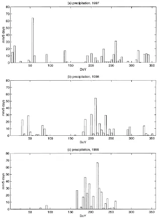
Fig. 2. Precipitation (mm per 5 day) measured on the Zapata grassland site during (a) 1997, (b) 1998 and (c) 1999.
et al., 1993; Giordani et al., 1996), and to represent the gravitational drainage (Mahfouf and Noilhan, 1996).
standing necromass Mn. The V–S model is driven by meteorological forcing variables, such as, air tem-perature, air humidity, wind speed, rainfall, and solar radiation. Additional surface characteristics, namely, soil parameters such as soil texture (% clay, % sand), soil thermal and hydraulic properties, root depth; and vegetation parameters such as SLA, maximum rate of photosynthesis are also prescribed (see Table 1).
3.2. Choice of the parameters, initialization and calibration
As stated in the introduction, one of our objectives in this study is to investigate the cost in terms of model calibration associated with the adaptation of a model developed and validated over a different site to a new site. A distinction needs to be made between the pa-rameters that can be found in the literature according to soil and/or vegetation classification and those that require on-site calibration.
3.2.1. Soil parameters
Several soil parameters are needed in order to spec-ify soil hydrological and thermal properties required by the SVAT model. For the site soil texture, the look-up table of (Clapp and Hornberger, 1978) indicates that the value of the soil moisture at field capacity (wfc) and at wilting point (wwp) are 0.195 and 0.114 m3m−3, respectively. However, the classification of Cosby et al. (1984) indicates that, for this soil type, the wilting point is equal to 0.065 m3m−3and the field capacity is contained between 0.12 and 0.22 m3m−3. Schmugge (1980) suggests another relation to estimate the field capacity as a function of soil texture, which leads to over the study site a value of 0.14 m3m−3. This value is inconsistent with the values of the maximum ob-served water content at the root zone in 1999, which represent an indirect way of estimating the soil mois-ture at the field capacity. In fact, the observed maxi-mum water content is close to 0.18 m3m−3in 1999. Based on the above consideration, an average value of 0.16 m3m−3forw
fcand of 0.065 m3m−3forwwp was adopted in this study. Concerning thermal con-ductivity, the approach described in Van de Griend and O’Neill (1986) has been implemented into the model. The model also requires appropriate coefficients for the soil resistance parameterization (Tables 1 and 2). In this regard, Chanzy, 1991 reported some difficulties
in establishing a one-to-one relationship between soil moisture and soil resistance to evaporation, even for a single soil type.
3.2.2. Surface and plant parameters
According to the measurements made by Nouvel-lon (1999) over the same site, 80–90% of root biomass is found in the first 30 cm of the soil. Measured av-erage minimal stomatal resistance and specific leaf area (SLA0) were 100 s m−1 and 30 m2kg C−1, re-spectively. Finally, the two phenological stages,j1and j2(i.e. growth and senescence timing) have been es-timated from the dynamics of the measurements of biomass in 1998 (see Table 1). The growth respiration coefficient for the above ground biomass was set to 0.49 g CO2g−1DM.
The model’s initialization depends on the initial amount of carbohydrate in the storage pool, and also on the rate at which this carbon is injected into the shoot and root compartments (initial carbon storage (IC) and Trans in Table 1). Since meteorological data during the first parts of the growing seasons were not
available, the model shoot carbon content had to be ini-tialized so as to match the biomass field measurements on the first day of the simulations for 1997–1999.
4. Assessment of the model performance
The V–S model has been run with measured at-mospheric forcing variables in conjunction with the
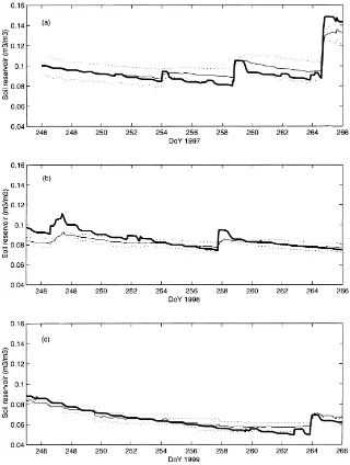
Fig. 4. Observed (–) and simulated ( ) hourly and half-hourly volumetric soil moisture in the root zone (m3/m3) for a 20-day period in 1997 (a), in 1998 (b) and in 1999 (c), respectively. The two time series of soil moisture measurements are plotted (· · ·).
From June to August, total rainfall in 1997 was about 127 mm while it was about 201 mm in 1998 and 304 mm in 1999. As a result, the biomass production was very low in 1997, average in 1998 and high in 1999. The peak biomass only reached 32 g DM m−2 in 1997 while it reached 72 g DM m−2 in 1998 and 113 g DM m−2 in 1999. The days corresponding to
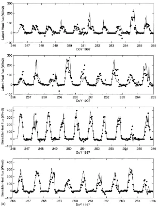
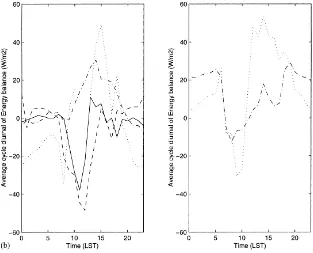
Fig. 5. (a) Simulated (–) and observed (d) hourly latent and sensible heat fluxes for a 20-day period of the 1997 growing season; (b) average diurnal cycle (local solar time) of the difference between measured and simulated components of the energy budget for the 1997 and 1998 growing seasons. Net radiation (–·), soil heat flux (· · ·), latent heat flux (–) and sensible heat flux (– –). Measurements of sensible and latent heat fluxes were not available for 1998.
Fig. 5 (Continued)
the short observation period. Maximum LAI was 0.32 in 1997, but it reached 0.4 in 1998 and 0.75 in 1999. Fig. 4 focuses on a 20-day period (day of year 246–265), and shows the dynamics of the simulated and observed hourly values (half hourly for 1999) of soil moisture in the root zone (w2) for all three study years. This period corresponds to the end of the rain season, and the grasses are usually at maximum de-velopment. The simulated soil moisture is within the range of TDR measurements, except for DoY 246–255 in 1998, when soil moisture is overestimated. This is mainly the result of model’s errors, which occur ear-lier in 1998 (the simulation starts at DoY 171 for this year). Such discrepancies were inherent to the use of the same set of parameters (soil resistance, field ca-pacity). This gives a reasonable agreement for the 3 years, although a year to year re-calibration can pro-duce better but less robust results. The 20-day period corresponds to a dry spell in 1999, although the simu-lated soil moisture is much higher than in 1997 when averaged over the whole growing season.
The time series of the simulated versus observed latent and sensible heat fluxes are shown in Fig. 5a for the same period of time. The root mean square error
(RMSE) between measured and simulated latent and sensible heat fluxes were 36 and 38 W m−2, respec-tively and therefore in good agreement. On Fig. 5b, we have represented the average diurnal cycle of the difference between the observed and estimated com-ponents of the energy balance for 1997 and 1998. There is a systematic bias around 11.00 h (LST) with an overestimation of the simulated latent and sensible heat fluxes. Given the errors associated with surface flux measurements in semi-arid regions, and the qual-ity of the energy balance closure, this bias is relatively small.
Fig. 6 (Continued) parameters, as highlighted by Cayrol et al. (in press).
Nevertheless, the previous evaluations show that the main features of the water and carbon dynamics are properly reproduced by the V–S model, which cap-tures the variability of plant response to the climate variability.
5. Ground and satellite data
The objective of this section is to assess the capabil-ity of the SPOT4-VEGETATION and NOAA/AVHRR sensors to track the temporal evolution of the vegeta-tion, and to address the questions 3 and 4 mentioned in Section 1.
Both ground measurements and model results pre-sented in the previous section indicate that the LAI of the Zapata grassland site is low (less than 0.8), and strongly variable over the timeframe of the study. Be-fore exploiting the coupling of remotely sensed data and models, we need to verify whether the seasonal evolution as well as the year to year variability of the vegetation is captured by satellite observations, even for such a low vegetation cover.
5.1. Ground-to-satellite approach
Fig. 7. NDVI time profile over the Zapata grassland, obtained from AVHRR (+) during (a) 1997 and (b) 1998 and from VEGETATION (s) during (b) 1998 and (c) 1999.
evolution. It is the latter corrected surface reflectances, which are used in the subsequent discussion.
The main objective in grassland monitoring is to estimate the evolution with time of the biomass using satellite data as surrogate measures. Scatter plots of LAI and biomass versus the SWIR and the RED re-flectance (Fig. 9a and b) reveal significant linear rela-tionships (Table 3). It is well-known that the green leaf
Fig. 8. Summertime reflectance (SWIR, NIR and RED reflectances) acquired by the VEGETATION sensor over the Zapata grassland in 1999. Bold symbols represent reflectances after correction for surface anisotropy effects.
scattering is partly caused by the residual noise, which still impairs the satellite time series. This noise seems to be larger for the SWIR than for the RED band (Fig. 8), and this may be related to the SWIR absorp-tion by the superficial soil moisture during the rain season (DoY 200–250). Another slight difference is that the RED reflectance increases gradually during the senescence period (270–320) whereas the SWIR increases more rapidly and plateaus around DoY 290.
Fig. 9. Scatter diagrams of the SWIR reflectance acquired by the VEGETATION sensor vs. the measured aboveground biomass and LAI during the two growing seasons (s), (e) and senescence periods (d), (r) of 1998 and 1999, respectively. The linear regressions are also plotted. Daily ’measurements’ of biomass and LAI are linearly interpolated from Figs. 1 and 3; (b) as in Fig. 9a except for the RED reflectance; (c) as in Fig. 9a except for the SWVI and NDVI vegetation indices.
in Fig. 9a–c). Not surprisingly, the regression are bet-ter for the LAI than for the biomass.
As far as we know, few studies, if any, have related the seasonal evolution of satellite-measured SWVI and vegetation characteristics, simply because the previ-ous AVHRR sensor did not record the reflectance in the SWIR (AVHRR channel 3 is also sensitive to the thermal emission). While these results are empirical, they are of interest since the impact on aerosol opti-cal depth is much smaller on the SWIR spectral band
than on the RED one. Since both wavelengths are sen-sitive to LAI, it is likely that a combined use of the SWIR, NIR and RED, also available on MODIS, may be more accurate than the former NIR and RED bands alone for vegetation monitoring.
5.2. Model-to-satellite approach
Fig. 9 (Continued)
Table 3
Correlations, slopes and intercepts of the linear relationships between VEGETATION reflectances (SWIR and RED), vegetation indices (SWVI and NDVI) and measured biomass and LAI collected over two years (1998 and 1999)
Biomass (g DM m−2)a LAI (m2m−2)a
SWIR −0.63 −0.68
−0.0005, 0.3048 −0.0755, 0.3046
RED −0.74 −0.76
−0.0005, 0.1586 −0.0677, 0.1572
NDVI 0.81 0.88
0.0026, 0.1505 0.3780, 0.1485
SWVI 0.76 0.86
0.0019,−0.1757 0.2991,−0.1832
(scattering by arbitrarily inclined leaves (SAIL); Ver-hoef, 1984) to compute surface reflectance in RED, NIR and SWIR regions (see Appendix C for more details). The central assumption is that the canopy reflectance depends on variables, green LAI, dead LAI, and can be computed by using SAIL and a set of
Fig. 10. (a) Comparison of the RED, NIR and SWIR reflectances simulated with the SAIL+V–S model and the normalized VEGETATION reflectances (s) over the Zapata grassland site in 1998 (the three figures on the left) and in 1999 (the three figures on the right). Simulations with the leaf optical properties from Walter-Shea et al. (1992) are in dashed line and solid line represents the simulation with the leaf optical properties from Asner et al. (1998); dotted lines are for the ’bright’ and ’dark’ parameter sets, see text); (b) as in Fig. 10a except for the vegetation indices, SWVI (s) and NDVI (+).
Fig. 10 (Continued)
from springtime VEGETATION data. Simulations errors were assessed by deriving a set of ‘bright’ opti-cal properties for green, yellow leaves and soil, and a set of ‘dark’ properties using the standard deviations (Tables 4 and 5). Fig. 10a presents the comparison between simulated and observed reflectances (RED, NIR and SWIR). For each wavelengths, one param-eter set or the other yielded a very good match to the VEGETATION data. However, here is no general agreement, because of the difference in the leaf
opti-Table 4
Variability of grass green leaf and litter optical properties in the VEGETATION bands (RED, NIR and SWIR)a
Reflectance Transmittance Reference
RED NIR SWIR RED NIR SWIR
Green leaf
0.097 (0.02) 0.38 (0.03) 0.29 (0.02) 0.04 (0.08) 0.34 (0.05) 0.31 (0.04) Asner et al. (1998)
0.1 0.45 0.3 0.05 0.5 0.4 Walter-Shea et al. (1992)
Litter leaf
0.43 (0.08) 0.53 (0.05) 0.5 (0.08) 0.13 (0.07) 0.22 (0.07) 0.25 (0.08) Asner et al. (1998)
0.25 0.43 0.3 – – – Walter-Shea et al. (1992)
aMean values from Asner et al. (1998) (standard deviations in parentheses) and mean values from Walter-Shea et al. (1992). The symbol – means no data available.
Table 5
Soil reflectance in the RED, NIR and SWIR bandsa
RED NIR SWIR
0.17 (0.0144) 0.23 (0.0168) 0.31 (0.0248) aValues (standard deviations in parentheses) from VEGETA-TION sensor before the growing 1999 season (DoY 160–175).
in 1999 (Fig. 10b), while the estimations of vegeta-tion indices with the data’s Walter–Shea are good. At this stage, the results show that there is a need to have robust estimates of the leaf optical properties, especially for multi-species canopies made of leaves and stems, and during the senescence period. With this caveat in mind, we conclude that the V–S model coupled to the SAIL scheme is able to reproduce the observed satellite reflectances, for the SWIR as well as for the RED and NIR reflectances.
This is an important step towards the use of the new satellite archives (VEGETATION, MODIS) within mechanistic vegetation models.
6. Concluding remarks
The first objective of this study was to analyze the capability of coupled Vegetation growth and SVAT models (V–S model) to reproduce the temporal evolu-tion of several variables measured at ground level dur-ing three growdur-ing seasons in the course of the SALSA program. These variables include grassland biomass and LAI, soil water content and various components of the energy budget. A second objective was to inves-tigate the potential of remotely sensed data to drive or control such a model, within the context of regional scale applications. Four questions, which address these two main objectives have been listed in the introduc-tion. Our conclusions based on the results of our anal-yses are as follows.
The V–S model used in this study was originally de-veloped for the Sahel environment. Its application to northern Mexico grasslands required some adaptations of the model, not in terms of the processes themselves, but for some of the parameters. For instance, the mini-mum stomatal resistance, the surface leaf area and the growth respiration rate were different for the SALSA grasses, according to ground measurements and liter-ature survey. Another difference between the Sahelian
annual grasses and the Mexican perennial grasses is the storage capacity of carbohydrate was set to a larger value for the latter. The soil characteristics, especially the water content at wilting point and field capacity were estimated according to Cosby et al. (1984). The use of different classifications, however, produced sig-nificantly different estimates, which were not always consistent with the soil moisture measurements. How-ever, the overall functioning including water and CO2 exchanges, was rather similar for the perennial Mexi-can grasslands and the annual Sahelian grassland, and the V–S model required few changes to simulate the growth, carbon and water balances.
The second question concerns the accuracy of the V–S model outputs. The energy balance and the veg-etation growth (biomass, LAI) were reasonably well simulated for the years 1997–1999. This 3-year test was satisfactory for the vegetation sub-model, which captures the large interannual variability, but it was less demanding for the energy sub-model because the intensive observation period was less extensive. The surface radiative temperature was well simulated for the three growing seasons. Overall, it is interesting to note that the V–S model performed relatively well, with the same parameter set, for strongly varying climatic conditions.
The third question deals with the ability of coarse resolution satellite to monitor the seasonal and inter-annual variability of vegetation status in semi-arid areas. Remotely sensed time series of NDVI and refle-ctance from the AVHRR and VEGETATION sensors successfully reflected the variability observed in biomass and LAI ground measurements, even for low values of the latter. Since the VEGETATION sensor records the surface short-wave infrared reflectance, individual relationships between LAI or biomass on the one hand, and the SWIR reflectance or a SWIR based vegetation index (SWVI) on the other hand could be established. These relationships were found to be linear for the low values of LAI of the Salsa grasslands. The SWIR and RED bands showed sim-ilar sensitivity to biomass and LAI. As a result, the SWIR based SWVI and the classical RED based NDVI produced very similar relationships.
The leaf optical properties were taken from two dif-ferent dataset. It was shown that the V–S model coupled to the SAIL scheme generally captures the seasonal evolution of the VEGETATION reflectances and spectral indices. For every spectral band, at least one of the input dataset lead to a good simulation of the observed satellite reflectance. However, uncer-tainties in the leaf optical properties, especially in the green leaf absorption in the NIR and in the dead tissues properties, resulted in large uncertainties in the NIR simulations. Robust estimates of the leaf, stems and litter parameters and of their variability are therefore highly desirable for regional scale applica-tions (e.g. through the validation network of the new sensors like MODIS). From the answers to these dif-ferent questions, it is concluded that the V–S model is suitable for long term modeling and monitoring of surface processes in arid and semi-arid areas. The physically-based model-to-satellite approach is promising, and the SAIL scheme seems also to be suitable for the SWIR band. Because this spectral do-main is known to be less sensitive to most aerosols, the VEGETATION and MODIS datasets may give a different view of the terrestrial ecosystems. Further work will consist in assimilating the satellite mea-surements at regional scales, with the objective of ob-taining accurate simulations of vegetation dynamics and surface energy budget over a large area.
Acknowledgements
This work and participation in the SALSA experi-ment were made possible through the support of the EC VEGETATION Preparatory Program and a Ph.D. grant from French MESR (Ministère de l’Enseigne-ment Supérieur et de la Recherche). Additional sup-port was provided by CONACyT and EOS-Project (NAGW2425). Many thanks are due to the many peo-ple involved in the impeo-plementation of the experiment in Mexico: Dr. Gilles Boulet, Dr. Chris Watts, Dr. J.-P. Brunel, Julio Rodriguez, O. Hartogensis, Mario Jauri and Saturnino Garcia. We would also like to thank Dr. Bruce Goff for helping us with the species identi-fication. Thanks also to G. Saint (CNES), CTIV and SPOT-image for helping us to access VEGETATION data. We are very grateful to Drs B. Berthelot and Ph. Maisongrande for processing of VEGETATION data
and to Dr. Malcolm Davidson for carefully reading the manuscript. The authors also express their deep grat-itude to the anonymous reviewers for their valuable comments and critical remarks.
Appendix A. Correction of the surface anisotropy
To remove the effect of surface anisotropy, we com-puted a normalized reflectance (Rnorm) using Eq. (A.1) from Wu et al. (1995)
Rnorm(Ao)=R(Aobs)×F with F = Rmod(Ao)
Rmod(Aobs)
(A.1)
where Ao is the reference or standard sun-sensor geometry (Table 6), Aobs is the actual sun-sensor geometry andF is the factor, which removes the di-rectional effects explained by a BDRF model. The BRDF model used is the AMBRALS model (Wanner et al., 1997) which is based on parameters kernel
Rmod=k0+k1f1(Aobs)+k2f2(Aobs) (A.2) where k0, k1 and k2 are free parameters obtained fitting Rmod to the data, f1 and f2 are the kernels, which are analytical functions of the sun and sensor zenith and azimuth angles. The first kernel aims at reproducing the volume scattering. The second ker-nel estimates the surface scattering and is based on geometrical approaches. We used the Ross-thick ker-nel with the Li-sparse kerker-nel. The surface reflectance may then computed for any sun-sensor geometry, e.g.
Table 6
Specification of the SAIL model input parameters
Canopy structure parameters
LAI As predicted by the
V–S model Leaf angle distribution Spherical (mean leaf
angle=57.30◦) Illumination and view conditions
Diffuse fraction of solar radiation 20%
Reference sun-target-sensora
View zenith angles 30◦
Solar zenith angles 30◦
Relative azimuth 140◦
the reference geometry (Ao). To account for a sea-sonal variation of the canopy properties, we used a ‘seasonal’ Ambral model
Rmod=Ka0+(1−K)a0′
+(Ka1+(1−K)a1′)f1(Aobs)
+(Ka2+(1−K)a2′)f2(Aobs) (A.3) wherea0,a1,a2 are the parameters corresponding to the ‘maximum vegetation season’ and the a′
0,a1′,a2′ are the parameters corresponding to the ‘minimum vegetation season’. The K coefficient is the NDVI, scaled between 0 and 1. This linear model is fitted to the 1998 and 1999 VEGETATION data and is used to provide normalized seasonal reflectances.
Appendix B. The V–S model’s main equations
Symbols and parameters values are listed in Table 1.
B.1. Daily time-step
B.1.1. Carbon balance
The dynamics of the three carbon compartments is described by a set of three differential equations
dMs
Eq. (B.1) expresses that the daily carbon increment of the shoots is the result of the carbon gain, photosynthe-sis (Pn) minus carbon lost during plant maintenance (msMs) and plant growth respiration (Rgs) and carbon losses due to senescencessMs. The carbon available for growth is partitioned between the shoot and roots according to the as allocation coefficient. The roots obey a similar equation Eq. (B.2), with a symmetric allocation coefficient (1−as).
The necromass dynamic depends on the difference between necromass production, which is equal to the shoot senescencessMs, and necromass decaysdnMn.
The LAI is computed from the shoots biomass and SLA according to a non-linear relationship that
accounts for the increasing importance of stems and other non-leaf tissues at high levels of biomass (relationship estimated from measurements Nouvel-lon, 1999) by the expression
SLA=0.0001[130.4
−332.5(1−exp(−0.0031nbj))] (B.4) where nbj is the number of day after the beginning of the growing season.
The carbon balance equations Eqs. (B.1)–(B.3) are solved on a daily basis, where as the photosynthesis (Pn) is computed and accumulated on an hourly basis. Indeed, it depends on the stomatal resistance, which is also involved in the SVAT model, and computed on an hourly (or half-hourly) basis.
B.1.2. Respiration and senescence
Following McCree (1970) and Amthor (1986, 1989) the total respiration consists of maintenance and growth respiration. The maintenance respiration is proportional to the biomass and its rate (ms or mr in Eqs. (B.1) and (B.2)) depends on air temperature according to a classicalQ10 relationship:
ms =ms0QT /1010 (B.5)
whereTis the daily average air temperature andms0is the respiration rate at 0◦C for the shoot (m
r0 for roots, respectively). The growth respiration is proportional to the amount of new tissue and therefore Eqs. (B.1) and (B.2) have to be rearranged as follows:
dMs
B.2. Hourly (or half hourly) time step
B.2.1. Stomatal resistance
The leaf stomatal resistance is of Jarvis’s (1976) type andrr are the stomatal and residual resistances (i.e. mesophyll diffusion and carboxylation resistances) to CO2transfer (e.g. Running and Coughlan, 1988). See Cayrol et al. (in press) for parameters derivations.
rr=rr ming1(I )g2(T )
B.2.3. Prognostic equations, surface fluxes and radiative temperature
The equations giving the evolution of the prognostic variables are
The energy balance is written separately for the soil and vegetation
Rng−LEg−Hg−G=0 (B.15)
and
Rnc−LEc−Hc=0 (B.16)
The network of resistances from Shuttleworth and Wallace (1985), between the soil surface, the within-canopy source level and the above-canopy ref-erence level allows to estimate the latent and sensible heat fluxes across differences in vapor pressure and temperature given by
The radiative temperature is expressed as follows:
Tr=
Appendix C. The SAIL model
Kubelka–Munk approximation to the radiative trans-fer equation (Goel, 1988). The model simulates the canopy spectral reflectance from LAI, leaf and soil optical properties, leaf angle distribution, acquisition geometry and diffuse part of the incoming solar radia-tion. The ratio between leaf size and vegetation height accounts for the hot-spot effect. The green and yellow LAI were predicted daily by the V–S model. The ge-ometric conditions correspond to the acquisition con-figurations (Table 6). The soil reflectances for visible, near infrared and short wave infrared were estimated from the first images of VEGETATION sensor before the beginning of the growing season (Table 5). Leaf optical parameters (Table 4) were prescribed for visi-ble, near infrared and short wave infrared from Asner et al. (1998) and Walter-Shea et al. (1992). A version of the SAIL model with two layers was used. Green vegetation was assumed to overtop dead leaves.
References
Amthor, J.S., 1986. Evolution and applicability of a whole plant respiration model. J. Theoritical Biol. 122, 473–490. Amthor, J.S., 1989. Respiration and Crop Productivity. Springer,
New York.
Asner, G.P., Wessman, C.A., Schimel, D.S., Archer, S., 1998. Variability in leaf and litter optical properties: implications for BRDF model inversion using AVHRR, MODIS and MISR, MODIS and MISR. Remote Sens. Environ. 63, 243–257. Avissar, R., 1995. Recent advances in the presentation of
land-atmosphere interactions in general circulation models. Rev. Geophys. 2, 1005–1010.
Bonan, G.B., Pollard, D., Thompson, S.L., 1992. Effects of boreal forest vegetation on global climate. Nature 359, 716–718. Braud, I., Noilhan, J., Bessemoulin, P., Haverkamp, R., Vauclin,
M., 1993. Bare-ground surface heat and water exchanges under dry conditions: observations and parameterization. Boundary Layer Meteorol. 66, 173–200.
Calvet, J.C., Noilhan, J., Rougean, J.L., Bessemoulin, P., Cabelguenne, M., Olioso, A., Wigneron, J.P., 1998a. An interac-tive vegetation SVAT model tested against data from six contrasting sites. Agric. For. Meteorol. 92, 73–95.
Calvet, J.C., Noilhan, J., Bessemoulin, P., 1998b. Retrieving the root-zone soil moisture or temperature estimates: a feasibility study based on field measurements. J. Appl. Meteorol. 37, 371– 386.
Cayrol, P., Kergoat, L., Moulin, S., Dedieu, G., Chehbouni, A., Calibrating a coupled SVAT/vegetation growth model with remotely sensed reflectance and surface temperature. A case study for the HAPEX-Sahel grassland sites. J. Appl. Meteorol., in press.
Chanzy, A., 1991. Modelisation simplifiée de l’évaporation d’un sol nu utilisant l’humidité et la temperature de surface accessibles
par télédétection. Thèse de docteur ingénieur agronome de l’Institut National Agronomique Paris-Grignon, France, p. 221. Choudhury, B.J., Monteith, J.L., 1988. A four layer model for the heat budget of homogeneous land surfaces. Q.J.R. Met. Soc. 114, 373–398.
Clapp, R.B., Hornberger, G.M., 1978. Empirical equations for some soil hydraulic properties. Water Resour. Res. 14 (4), 601–604. Cosby, B.J., Hornberger, G.M., Clapp, R.B., Ginn, T.R., 1984. A statistical exploration of the relationships of soil moisture characteristics to the physical properties of soils. Water Resour. Res. 20, 682–690.
Deardorff, J.W., 1978. Efficient prediction of ground surface temp-erature and moisture, with inclusion of a layer of vegetation. J. Geophys. Res. 83, 1889–1903.
DeVries, D.A., 1963. Thermal properties of soils. In: Van Wijk, N.R. (Ed.), Physics of Plant Environment. Holland Publishing, Amsterdam.
Dickinson, R.E., Shaikh, M., Bryant, R., Graumlich, L., 1998. Interactive canopies for a climate model. J. Climate 11, 2823– 2836.
Giordani, H., Noilhan, J., Lacarrère, J., Bessemoulin, P., 1996. Modeling the surface processes and the atmospheric boundary layer for semi-arid conditions. Agric. For. Meteorol. 80, 263– 287.
Goel, N.S., 1988. Models of vegetation canopy reflectance and their use in estimation of biophysical parameters from reflectance data. Remote Sens. Rev. 4, 1–212.
Goodrich, D.C., Chehbouni, A., Goff, B., MacNish, B., Maddock III, T., Moran, M.S., Shuttleworth, W.J., Williams, D.G., Watts, C., Hipps, L.H., Cooper, D.I., Schieldge, J., Kerr, Y.H., Arias, H., Kirkland, M., Carlos, R., Cayrol, P., Kepner, W., Jones, B., Avissar, R., Begue, A., Bonnefond, J.-M., Boulet, G., Branan, B., Brunel, J.P., Chen, L.C., Clarke, T., Davis, M.R., DeBruin, H., Dedieu, G., Elguero, E., Eichinger, W.E., Everitt, J., Garatuza-Payan, J., Gempko, Gupta, H., Harlow, C., Hartogensis, O., Helfert, M., Holifield, C., Hymer, D., Kahle, A., Keefer, T., Krishnamoorthy, S., Lhomme, J.-P., Lagouarde, J.-P., Lo Seen, D., Laquet, D., Marsett, R., Monteny, B., Ni, W., Nouvellon, Y., Pinker, R.T., Peters, C., Pool, D., Qi, J., Rambal, S., Rodriguez, J., Santiago, F., Sano, E., Schaeffer, S.M., Schulte, S., Scott, R., Shao, X., Snyder, K.A., Sorooshian, S., Unkrich, C.L., Whitaker, M., Yucel, I., 2000. Preface paper to the semi-arid land-surface-atmosphere (SALSA) program special issue. Agric. For. Meteorol. 105, 3–19.
Gupta, H.V., Sorooshian, S., Yapo, P.O., 1998. Toward improved calibration of hydrologic models: multiple and non commensurable measures of information. Water Resour. Res. 34 (4), 751–763.
Hunt Jr., E.R., Rock, B.N., 1989. Detection of changes in leaf water content using near- and middle-infrared reflectances. Remote Sens. Environ. 30, 43–54.
Jarvis, P.G., 1976. The interpretation of the variations in the leaf water potential and stomatal conductance found in canopies in the field. Phil. Trans. R. Soc. London, Ser. B 273, 593–610. Kergoat, L., 1998. A model for hydrological equilibrium of leaf
area index on a global scale. J. Hydrol. 212/213, 268–286. Kustas, W.P., Prueger, J.H., Humes, K.S., Starks, P.J., 1999.
layer versus mixed-layer atmospheric variables with radiometric temperature observations. J. Appl. Meterol. 38, 224–238. Le Roux, X., 1995. Etude et modélisation des échanges d’eau et
d’énergie sol-végétation-atmosphére dans une savane humide (Lamto, Côte d’Ivoire). Thèse de l’université Pierre et Marie Curie, Paris, France, p. 203.
Lo Seen, D., Chehbouni, A., Njoku, E.G., Saatchi, S., Mougin, E., Monteny, B., 1997. A coupled biomass production, water and surface energy balance model for remote sensing application in semiarid grasslands. Agric. For. Meteorol. 83, 49–74. Mahfouf, J.F., Noilhan, J., 1996. Inclusion of gravitational drainage
in a land surface scheme based on the force-restore method. J. Appl. Meteorol. 35 (6), 987–992.
Mahrt, L., Ek, M., 1984. The influence of atmospheric stability on potential evaporation. J. Clim. Appl. Meteorol. 23, 222– 234.
McCree, K.J., 1970. An equation for the rate of respiration of white clover plants grown under controlled conditions. In: Setlik, I. (Ed.), Prediction and Measurement of Photosynthetic Productivity. Proceedings of the IBP/PP Technical Meeting, Trebon, PUDOC, Wageningen, The Netherlands, pp. 221– 229.
Nobre, C.A., Sellers, P.J., Shukla, J.U., 1991. Amazonian defo-restation and regional climate change. J. Climate 4, 957–987. Nouvellon, Y., 1999. Modélisation du fonctionnement de prairies
semi-arides et assimilation de données radiométriques dans le modèle. Thèse de docteur ingénieur agronome de l’Institut National Agronomique Paris, France.
Nouvellon, Y., Rambal, S., Lo Seen, D., Moran, M.S., Lhomme, J.P., Bégué, A., Chehbouni, A.G., Kerr, Y., 2000. Modelling of daily fluxes of water and carbon from shortgrass steppes. Agric. For. Meteor. 100, 137–153.
Passerat de Silans, A., 1986. Transferts de masse et de chaleur dans un sol stratifié soumis à une exitation atmosphérique naturelle. Comparaison modèle expérience, Thèse de l’institut National de Polytechnique de Grenoble, France, 205 p.
Pielke, R.A., Liston, G.E., Lu, L., Vidale, P.L., Walko, R.L., Kittel, T.G.F., Parton, W.J., Field, C.B., 1997. Coupling of land and atmospheric models over the GCIP area — CENTURY, RAMS, and SIB2C, 2–7 February 1997, LongBeach, CA (preprint of the 13th Conference on Hydrology).
Running, S.W., Coughlan, J.C., 1988. A global model of forest ecosystem processes for regional applications. Hydrological balance canopy gas exchange and primary production processes. Ecol. Model. 42, 125–154.
Schmugge, T.J., 1980. Effect of texture on microwave emission from soils. IEEE Trans. Geosci. Rem. Sensing, GE 18 (4), 353–361.
Shuttleworth, W.J., Gurney, R.J., 1990. Evaporation from sparse crops — an energy combination theory. Q.J.R. Met. Soc. 111, 839–855.
Shuttleworth, W.J., Wallace, J.S., 1985. The theoretical relation-ships between foliage temperature and canopy resistance in sparse crops. Q.J.R. Met. Soc. 116, 497–519.
Stannard, D.I., Blanfort, J.H., Kustas, W.P., Nichols, W.D., Amer, S.A., Shummge, T.J., Weltz, M.A., 1994. Interpretation of surface flux measurements in heterogeneous terrain during the Monsoon’90 experiment. Water Resour. Res. 30, 1227–1239. Van de Griend, A.A., O’Neill, P.E., 1986. Discrimination of soil
hydraulic properties by combined thermal infrared and micro-wave remote sensing. In: Proceedings of the IGARSS’86 Sym-posium, Vol. 254, Zurich, 8–11 September 1986. ESA SP, pp. 839–845.
Verhoef, W., 1984. Light scattering by leaf layers with application to canopy reflectance modeling: the SAIL model. Remote Sens. Environ. 16, 125–141.
Walter-Shea, E.A., Blad, B.L., Hays, C.J., Mesarch, M.A., 1992. Biophysical properties affecting vegetation canopy reflectance and absorbed photosynthetically active radiation at the FIFE site. J. Geophys. Res. 97 (D17), 18925–18934.
Wanner, W., Strahler, A.H., Hu, B., Muller, J.P., Li, X., Barker Schaaf, C.L., Barnsley, M.J., 1997. Global retrieval of bidirec-tional reflectance and albedo over land from EOS MODIS and MISR data: theory and algorithm. J. Geophys. Res. 102, 17143–17161.
Williams, G.J., Markley, J.L., 1973. The photosynthetic pathway type of North American shortgrass prairie species and some ecological implications. Photosynthetica 7 (3), 262–270. Wu, A., Li, Z., Cilhar, J., 1995. Effects of land cover type