NEW DTM EXTRACTION APPROACH FROM AIRBORNE IMAGES DERIVED DSM
Yousif Abdul-kadhim Mousa a, b*, Petra Helmholz a, David Belton a
a Department of Spatial Sciences, Curtin University, Perth, WA, Australia – a [email protected], [email protected], [email protected] b Al-Muthanna University, College of Engineering, Civil Engineering department, Al-Muthanna, Iraq
Commission II, WG II / 4
KEY WORDS: Digital Surface Model (DSM), Digital Terrain Model (DTM), DTM extraction, normalised DSM (nDSM), airborne images, LiDAR
ABSTRACT:
In this work, a new filtering approach is proposed for a fully automatic Digital Terrain Model (DTM) extraction from very high resolution airborne images derived Digital Surface Models (DSMs). Our approach represents an enhancement of the existing DTM extraction algorithm Multi-directional and Slope Dependent (MSD) by proposing parameters that are more reliable for the selection of ground pixels and the pixelwise classification. To achieve this, four main steps are implemented: Firstly, 8 well-distributed scanlines are used to search for minima as a ground point within a pre-defined filtering window size. These selected ground points are stored with their positions on a 2D surface to create a network of ground points. Then, an initial DTM is created using an interpolation method to fill the gaps in the 2D surface. Afterwards, a pixel to pixel comparison between the initial DTM and the original DSM is performed utilising pixelwise classification of ground and non-ground pixels by applying a vertical height threshold. Finally, the pixels classified as non-ground are removed and the remaining holes are filled. The approach is evaluated using the Vaihingen benchmark dataset provided by the ISPRS working group III / 4. The evaluation includes the comparison of our approach, denoted as Network of Ground Points (NGPs) algorithm, with the DTM created based on MSD as well as a reference DTM generated from LiDAR data. The results show that our proposed approach over performs the MSD approach.
1. INTRODUCTION
Having an accurate and reliable DTM is beneficial for numerous mapping applications in photogrammetry and remote sensing, such as object detection. High resolution stereo images from airborne or satellite platforms can achieve sub-meter Ground Sample Distance (GSD) and therefore have yielded the opportunity to produce a high resolution and accurate Digital Surface Models (DSMs) by using dense image matching technique (Hirschmuller, 2008). In the context of this paper a DSM is defined including all visible ground details, i.e. the visible terrain and all objects such as buildings and trees on the terrain. Therefore, a DSM can be separated into a Digital Terrain Model (DTM) representing the bare ground including roads and low vegetation, as well as a normalized DSM (nDSM) describing non-ground objects such as buildings and vegetation. However, the extraction of reliable DTMs from DSMs is not a straight forward process, and is an ongoing research topic especially with respect to densely built-up areas (Krauß et al., 2011).
The two most common approaches to generating DSMs are based on images using stereo image matching techniques and Light Detection and Ranging (LiDAR). Recently, state-of-the-art dense image matching approaches such as Semiglobal Matching SGM (Hirschmuller, 2008) have been considered to generate high resolution and accurate DSM for object detection and 3D reconstruction (Bulatov et al., 2014). However, DSM derived from stereo image matching often contains holes as a result of occlusion and mismatches (Krauß et al., 2015). Such holes can be filled by interpolation (Krauß & d’Angelo, 2011). As a result, sharp edges e.g. building boundaries might be smoothed. In contrast, LiDAR data yields more well defined DSMs and the objects outlines are well defined (Perko et al., 2015; Tian et al., 2014).
This research proposes a robust DTM extraction algorithm for DSMs derived from very high resolution airborne images in structurally complex regions. The basic idea is to enhance the approach of (Perko et al., 2015) by adding additional parameters for the selection of the minimum ground points and the pixelwise classification. Furthermore, instead of applying the complex and non optimal local slope correction of (Perko et al., 2015), an alternative technique is proposed. This technique is
simpler, more reliable and faster, which is based on creating a network of ground points (NGPs). In addition, our approach will not be affected by the smoothed transition caused by occlusion during the generated DSM process as the slope angle threshold is eliminated from the pixelwise classification process completely.
This paper is structured as followed. The related studies are reviewed and discussed in the next section. Then, we explained our approach in detail in the third section. In the fourth section, the approach is evaluated; results are shown and analysed. The last section concludes the paper and outlines future work.
2. PREVIOUS WORK
Based on the literature, there are a limited DTM extraction methods in the context of photogrammetric DSMs when compared with LiDAR-based DTM extraction methods (Beumier & Idrissa, 2016). A good review about DTM extraction algorithms for LiDAR data can be found in (Meng et al., 2010). More generally, the authors classified ground filtering algorithms into six major categories including Segmentation and Clustering, Morphological, Directional Scanning, Contour, Triangulated Irregular Network (TIN), and Interpolation. In contrast, our work targets DTM extraction from DSMs based on photogrammetry. However, while DSMs derived from airborne or very high satellite stereo images are in general similar to DSMs derived from LiDAR, the main exception is the spatial resolution (point density). DSMs derived from images generally have a higher spatial resolution but less accuracy in height measurements (Beumier & Idrissa, 2016). Fusion of images information with DSMs could be a useful option for DTM generation. However, the variety of the man-made objects and their occurrence mitigates the anticipated benefits (Beumier & Idrissa, 2016). For these reasons our literature review is limited to approaches designed for automatic DTM extraction from only photogrammetry-based DSMs.
A Morphological Filters approach is proposed by Haralick et al. (1987) and Förstner (1982) and is based on the idea that -DSMs can be represented as a grayscale image with its pixel values indicating a height value. Treating the DSM as a grayscale image gives the opportunity to apply image processing technologies which can remove high (bright) areas from the The International Archives of the Photogrammetry, Remote Sensing and Spatial Information Sciences, Volume XLII-1/W1, 2017
DSM. Namely, an opening filter consisting of erosion and dilation are used to eliminate non-ground points (e.g. buildings) from the DSM. For instance, (Krauß et al., 2011) first applies a minimum filtering with an approximated filter size higher than the cross section of a building. In this context, the filter size (diameter) is called a structural element (SE). As a result, all pixels containing non-ground information, e.g. roof pixels are replaced by minimum ground elevation heights within the SE. Next, a maximum filtering (dilation) is applied to restore edges of eroded terrain points. The main disadvantage of this method is the failure for DSMs containing roof objects smaller or larger than the implemented SE. Additionally, applying only classical opening on noisy DSMs containing negative outliers values leads to dominate these negative values in the resulting DTM (Krauß et al., 2011). Krauß et al. (2008) overcomes the noisy DSMs problem by applying low and high rank median filters instead of the erosion and dilation filters respectively. However, the decision of the rank of the low pass filter (e.g. 3%, 4% or 5%) depends on the applied filter size SE and the density of the built-up areas within the area of interested. Therefore, manual iterative parameter estimation is required. Furthermore, this low-rank percentage might correspond to non-ground regions, especially in high density built up areas e.g. on top of buildings, leading to dominate non- ground values in the resulting DTM. Or, vice versa, this low percentage might belong to too low bare-ground regions leading to dominate too low values.
Arefi et al. (2009) proposed a DTM extraction method named Geodesic Dilation which applies a vertical height threshold instead of the horizontal opening threshold. Again, as in the previous approach, the grey values correspond to the elevation heights. Two equal size images are required called mask (J) and marker image (I). The marker image grey values’ must be less than or equal to the mask image grey values’. The marker image is generated according to:
, = { , ,min , � , otherwise ℎ
That means that the marker image has the same elevation values as the mask on its border and all other marker’s pixels have one value correspond to minimum value from the mask. At the beginning, the mask image has the same value as the original DSM. For each pixel in the evaluation process, 4 directional filters are conducted from each corner to the opposite site of the image, i.e. from upper left (UL) corner to lower right (LR), from LR to UL, from upper right (UR) to lower left (LL) and from LL to UR. For each evaluation process, three pixels values from the marker are compared with three pixels values from the mask along the scanline direction, and the height difference between them is calculated. A scanline denotes a one directional line where there are a number of pixels are positioned along the line within a specific window size in the raster DSM. Non-ground objects are identified if the height difference is larger than a pre-defined threshold. However, when buildings are positioning close to the border of the image, the height difference is often lower than the threshold depending on the object surface properties. This can create non-satisfactory filtering result, especially in high resolution DSMs. Furthermore, the height difference between pixels belonging to raised bare-ground regions form the mask with their connected pixels from the marker is might be higher than the threshold, especially in sloped areas. As a result, these raised ground pixels will be eliminated from the resulting DTM.
Krauß and Reinartz (2010) proposed a DTM extraction method called Steep Edge Detection. The idea is to apply two median filters with different filter sizes. The different filter sizes will show the occurrences of various sharp ends. For instance, a larger dimension median filter fills up small holes while a smaller median filter tracks the elevation structure of the original DSM more precisely. Afterwards, the median filter results are subtracted from each other using a vertical threshold set to the lowest values for possible sharp edges. The resulting regions normally correspond to the bare-ground regions which
are then filled and interpolated to create the DTM. The main drawback of this method is that when some large objects are located on the building roofs, these objects maybe confused with buildings instead of being identified as part of the buildings leading to the lower roof pixels being incorrectly detected as ground pixels (Krauß et al., 2011). Secondly, when low vegetation such as small bushes are located in close proximity to buildings, these bushes might be also taken as ground points leading to decrease the accuracy of the generated DTM.
Perko et al. (2015) developed a new DTM extraction algorithm for DSMs derived from very high resolution satellite images called Multi-directional and Slope Dependent (MSD). This algorithm is an extension of the directional filtering approach introduced by (Meng et al., 2009). The main idea of the MSD algorithm is to specify points in the derived DSM which are positioned on bare ground regions and eliminate all other non-ground points. First of all, a robust slope fitting is performed using 2D Gaussian smoothing filter in order to smooth and correct the local slope terrain. Then, points located on bare ground regions are determined by applying 4 directional scanlines which intersect at the pixel under evaluation in the middle of a pre-defined window (Figure 2a). The dimension of the window is defined by the filtering size. For each scanline in this window, the pixel value with the minimum elevation value is selected. During the evaluation process, the elevation of the point under examination is compared to this minimum value. If the height difference is larger than a pre-defined height threshold, the pixel under examination is classified as a non-ground point. Otherwise, the slope difference between the current and the following pixel in the scanline direction will be calculated. If the slope is greater than a pre-defined slope threshold, this point is also labelled as a non-ground point. If the slope is less than the slope threshold and positive, the point is classified the same as the label of the previous point. If the slope is less than the slope threshold and negative, the point is labelled as a ground point. The process is repeated for all 4 scanlines in two directions leading to a total of 8. Finally, a pixel is classified as a ground point if the results of more than five labels indicated this point as a ground point. Otherwise, the point is classified as a non-ground point.
Beumier and Idrissa (2016) developed a DTM extraction method from DSMs based on photogrammetry. As a pre-processing step, the input DSM is smoothed using a Mean-shift filter. Then, the segmentation followed by region filtering are implemented and repeated. The segmentation technique is implemented for separating the DSM into regions based on the height information. The region filtering is applied for rejecting parts that are locally higher, which typically corresponds to non-ground objects such as buildings depending on neighbourhood analysis. The remaining regions are normally match roads, large surface or fields. Finally, holes resulted from rejecting non-ground objects in the previous step is then interpolated using bilinear interpolation technique to generate final DTM.
According to Meng et al. (2010) classification, the approach introduced by Beumier and Idrissa (2016) belongs to segmentation category. By contrast, our development approach is positioned in the context of directional scanning category. Hence, the next section will discuss the advantages and disadvantages of the directional scanning algorithms focusing on the MSD method because it belongs to the same class and in the context of DSMs based on photogrammetry.
3. METHODOLOGY
Based on the discussion of the main drawbacks of the MSD algorithm, we will introduce our NGPs method in detail, and will outline the different steps involve to improve its ability of overcome these drawbacks.
3.1 Problem Statement
Generally, three major steps are required to extract a DTM from a DSM following the MSD method (Perko et al., 2015):
1. Selecting pixels in the input DSM positioned on bare-ground areas.
2. Eliminating all other non-bare-ground areas. 3. Filling holes using an interpolation method.
Drawback 1: No ground points in the scanlines
According to (Perko et al., 2015), the most critical step of the approached is the determination of pixels that are positioned on the bare-ground areas. For each scanline within the extent of the filter area, a minimum of one point is required to be determined as belonging to the ground. The first drawback is given in the case that none of the points in the scanline is actually located on a bare-ground region is considered. However, this is easily possible and depends on the complexity of the structure in the area of interest, e.g. density of the built-up area, large building dimensions, very high resolution DSMs and the used filter size. If incorrect points are selected as minima, it will result in the incorrect classification of all other pixels within the filter size. Extending the filter size and therefore the length of the scanlines is not an ultimate solution to the problem because it can lead to some raised bare-ground pixels being incorrectly classified as a non-ground pixel, especially if the area of interest is not flat. Consequently, incorrect;y choosing the minimal value will influence the DTM extraction negatively.
Drawback 2: Selection of correct minima in sloped areas The second drawback is related to the local slope correction, or in otherwords, the determination of correct minima in sloped areas. (Perko et al., 2015) uses terrain slope fitting by applying a 2D Gaussian smoothing filter to solve this problem. However, such drawback cannot be overcome optimally in this way as the input DSM values were manipulated by the smoothing step. As a result, the incorrect choosing of minimal values could also occur in this case.
Drawback 3: Slope angle as a measure in high resolution DSMs Assuming that the minimum point was determined correctly, the third drawback is given when the height difference w.r.t. the currently evaluated pixel is less than a pre-chosen vertical threshold in all directions. In this case, slope differences between the current and the following pixel in the scanline direction will be considered to make a classification decision whether the pixel is a ground or non-ground pixel. This drawback is especially present in high resolution DSMs as they are common when extracted from airborne images. Figure 1 shows the pixel under evaluation in the centre highlighted in grey with its neighbours in original DSM (Figure 1a also called oDSM) and in the smoothed DSM (in Figure 1b also called sDSM) after the 2D Gaussian filter was applied. The evaluated pixel in the centre should get the classification result “ground point” as can be seen by the height values in the figure. Let’s assume that the previous pixels are classified as ground pixels, the slope threshold is set to 30 degree, and the GSD equals 0.14 m. All of the assumptions are likely for a DSM of a city with some slopes. For the example in Figure 1a, the difference of the scanline pixel in the top left corner to the currently evaluated pixel in the centre (oDSMDiff) is:
���� = . − . = . m
And analogue for the smooth DSM sDSMDiff is:
���� = . − . = − . m
Calculating the difference of oDSMDiff and sDSMDiff gives us:
∆ = ���� − ��� � = − . (1)
For the scanline running horizontally between the evaluated pixel and the left side, Δ is 0.047m and Ʌ is -18.5535 degrees. As Ʌ is smaller than the pre-defined threshold (and smaller than zero) the given label would be “ground point”. Similarly, the local slope Ʌ between the evaluated pixel and the bottom left scanline is 10.7155 degrees, and will be labelled similarly to the previous pixel “ground point” with Ʌ being smaller than the threshold. When continuing with calculating the slopes to all directions, the label “ground point” is given 3 times and the label “non-ground point” is given 5 times. Accordingly, the evaluated pixel in the centre will be classified as a non-ground pixel. Increasing the slope threshold to e.g, 60 degrees is not an optimal solution because 60 degrees corresponds to a height change equal to 24cm over a 14cm distance. These height changes are unlikely to appear everywhere without transitioning areas from ground to non-ground or vice versa. As a conclusion: The slope angle as a measure introduced in (Meng et al., 2009; Perko et al., 2015) seems to be not suitable for the DTM generation based on DSMs with a resolution of less than 1m GSD. For this reason the slope angle measure will be excluded from the processing of DTM extraction in our approach and will be replaced by an alternative solution.
(a) (b)
1. Designing a new filter structure in such way that well-distributed ground points are selected.
2. Adding a vertical threshold for choosing minimum pixels to be accepted.
3. Building a network of accepted ground points as minima and storing them with their geo-reference positions of the original DSM in a 2D surface. 4. Creating an initial DTM using an interpolation
method to fill the gaps between the created NGPs in the 2D surface.
5. Pixel to pixel comparison between the initial DTM and the original DSM for pairwise classification of ground and non-ground pixel by applying a second vertical threshold.
6. Finally, removing non-ground pixels and filling the remaining holes.
As one of the main contributions of the enhancement is the network of ground points, we will refer to the NGPs algorithm as our new proposed method.
First of all, if the input DSM contains outliers due to occlusion or mismatches, these outliers have to be removed. These areas and gaps then have to be filled with an interpolation method.
To overcome the first drawback, a new parameter is proposed to examine all points selected as minima in all executed scanlines. For example, for each executed scanline, there is one point selected as a ground point because it has a minimum value. The values of these points are sorted, and the first minimum value is eliminated in order to avoid points from too lower regions due to mismatches and the second value will be accepted instead. Afterwards, the height differences between the accepted point (second) and each of the remaining points are computed. If the height difference of a point is smaller than a pre-defined vertical threshold (1.1m in our case study), this point is also accepted. The International Archives of the Photogrammetry, Remote Sensing and Spatial Information Sciences, Volume XLII-1/W1, 2017
Otherwise, it will be eliminated from the process because it might be a non-ground point.
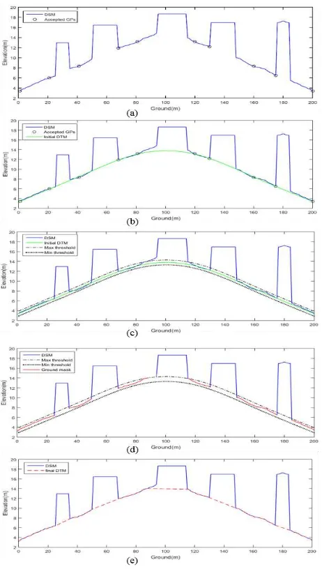
To overcome the second and third drawbacks in a more reliable manner, a novel technique is proposed. In order to reduce the computation procedure we work on the input DSM (i.e. no smoothing is applied) to obtain well-distributed ground points (GP). Furthermore, in addition to the 4 scanlines proposed in the MSD approach (Figure 2a), another 4 scanlines are proposed given us a total of 8 scanlines (Figure 2b) which yielded 8 points. Pixels highlighted in an orange are excluded from the process to avoid scanlines sharing the same pixel as minimal values. The 8 points will be examined before they are accepted as a ground point as discussed previously. Figure 3a is shown of the original DSM which we estimated initial ground pixels from the previous step. Then, the accepted ground points are stored with their geo-reference position to build a network of ground points (NGPs) for one scanline. Further, an initial DTM is generated by filling the gaps between the created NGPs (Figure 3b). Afterwards, a vertical pixel to pixel comparison between the initial DTM and the original DSM is performed by applying a vertical threshold shown in figure 3c. If the height difference is less than the chosen vertical threshold (e.g. absolute 0.4m), this pixel is classified as a ground pixel, otherwise, it is a non-ground pixel. These classified non-ground pixels correspond to the ground mask shown as a red line in Figure 3d. Finally, the remaining gaps between the ground mask are filled through interpolation shown as a dash red in figure 3e. Because the pixel to pixel vertical height threshold between the initial DTM and the original DSM is a more reliable measure than the slope threshold, the NGPs algorithm is a powerful alternative solution.
Figure (2). Directional scanlines for minimum point selection (a) MSD approach and (b) NGPs approach.
4. EVALUATION 4.1 Dataset
For the evaluation, the Vaihingen (Germany) dataset provided by the former ISPRS working group III / 4 is used. This test dataset was chosen because:
the images were captured with high resolution airborne cameras,
reference data in the form of airborne laser scanning (ALS) data are available; and
the data represent a complex scene of a high dense urban area with many buildings, vegetation and cars as well as a slope of the terrain.The specifications of the dataset are as followed:
Airborne images (8 cm GSD) associated with their orientation parameters; acquired using the platform Intergraph/ZI DMC with 0.12 m focal length (Cramer, 2010). The colour information consists of three bands: near infrared (NIR), red (R), and Green (G). The derived true orthophoto mosaic is provided.
Airborne Laser Scanning (ALS) data captured using a Leica ALS50 system with 4 points/m2 density average and its derived DSM with 25 cm GSD.
Digital surface models (DSMs) generated by dense matching using the Match-T software with 14 cm and 9 cm spatial resolution.
From this dataset, we especially focus on area 1 (“Inner City”) and area 2 (“High Riser”). While area 1 is especially suitable
due to the sloped terrain covered with a complex irregular building structure including vegetation, area 2 was selected because of the existence of high raised buildings with larger objects located on top of some of those buildings.
Figure (3). Logical steps of DTM generation by NGPs algorithm. Ground points (GPs) selected as minima on an artificial DSM (a), initial DTM (b), and vertical threshold limits (c), ground mask (d), and final DTM (e).
4.2 Parameter settings
The parameters used for the MSD approach are provided in Table 1, and for the NGPs approach accordantly in Table 2; the same parameters were used for both areas. The values for the filtering window size are fixed to 53m for both approaches and both tests. The filtering window size is based on the dimensions of the buildings in the scene. For the MSD approach, the height threshold is based on the absolute height difference between ground and buildings while the slope threshold is based on the height difference between the centre pixel and the one in scanline direction as well as on GSD. Regarding the NGPs approach, the first vertical threshold is based on the height difference between ground points selected as a minimum from different scanline. For non-flat areas, the value for this threshold should be increased by increasing the filtering window size and the angle of slope and vice versa. The second vertical threshold is based on the vertical height difference between the initial DTM and the original DSM. Increasing this threshold means capturing higher regions located between ground and non-ground regions.
Filter size 53 m
Height threshold 3 m
Slope threshold 30
Table 1. Parameters’ values (MSD approach).
Filter size 53 m
Vertical threshold for accepting ground points 1.1 m Vertical threshold for detecting ground mask 0.4 m Table 2. Parameters’ values (NGPs approach).
For the creation of the nDSMs for both approaches and test sets a threshold of 2m is applied, i.e. only objects with a height of more than 2m is shown in the nDSMs.
4.3 Qualitative Evaluation
4.3.1 Area1: Figure 4 shows DSM derived from ALS data (a) and a reference DTM (b). The resulting DTMs using the MSD algorithm and the NGPs algorithm are presented in Figure 5. The Figure shows the ortho image for Area 1 (a), the DSM with 14cm GSD based on image matching (b), the detected ground regions mask (c), the resulting DTM (d) and the created nDSM (e) using the MSD algorithm as well as the network of ground points accepted as minima values (f), the initial DTM (g), the detected ground regions mask (h), the extracted DTM (i) and the resulting nDSM using the NGPs algorithm (j).
Obviously, when comparing the results of the ground masks (Figures 5c and h), details are lost by MSD approach as highlighted with yellow circles (Figure 5c), while larger regions belonging to bare-ground are successfully detected by the NGPs approach (Figure 5h). The NGPs approach is able to segment buildings, high vegetation, and even some cars, and excluded them from the ground mask.
Furthermore, the second last row of images in Figure 5 show the resulting DTMs. There is one highlighted area in the generated DTMs of the MSD approach (Figures 5d) as well as in the NGPs approach (Figure 5i). This area indicates an error in the generated DTM whereas instead, it is actually due to an error in the input DSM. The cause of this error is unknown but can be seen more clearly in Figure 4. While in the LiDAR dataset a building within the highlighted area is clearly visible (Figure 4a), this area is classified as terrain in the DTM processed by LAStool (Figure 4b).
Lastly, the normalised DSMs (also called nDSMs) are presented in the last row of Figure 5. The nDSMs are created by subtracting DTM from DSM. Then, by thresholding the nDSM (above 2m), all non-ground point, i.e. buildings and high vegetation will be obtained. The differences are clearly visible and are highlighted in the figure. While many raised bare-ground regions were not detected by the MSD approach leading to a cluttered nDSM (Figure 5e), the nDSM created by NGPs represents the location of buildings more realistic (Figure 5j). This is mainly due to the successful identification of ground points (Figure 5f).
Figure 4. Area1 DSM derived from LiDAR data (a) and the reference DTM (b).
Figure 5. Ortho image for area1 (a) and input DSM (b). Ground mask (c), DTM (d), and nDSM (e) by MSD method. Network of ground points (f), initial DTM (g), ground mask (h), final DTM (i), and nDSM (j) by NGPs method.
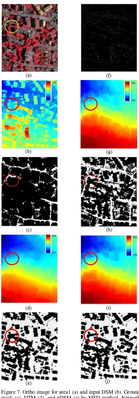
4.3.2 Area2: DSM derived from ALS data (a) and a reference DTM (b) are shown in Figure 6. Figure 7 presents the outputs of both algorithms. The Figure shows the ortho image for Area 2 (a), the DSM of 9cm GSD based on image matching (b). The resulting ground masks, DTMs and nDSMs are in the same order as for area 1.
The difference in the created ground masks of the MSD approach (Figure 7c) to the NGPs approach (Figure 7h) is clearly visible. For instance, wide ground regions have been lost from the ground mask using the MSD approach and non-ground points are clustered together. In contrast, our proposed algorithm NGPs successfully detects those areas.
Figures 7d and 7i show the DTMs created by MSD and NGPs approaches respectively. Both DTMs seem to be similar except the areas highlighted with red circles. NGPs DTM values in this area are clearly higher than the DTM created by MSD and even higher than LiDAR DTM as highlighted in figure 6b. In fact, the true height value for this ground area is higher than all created DTMs, as visible in the ortho image (Figure 7a) and in the DSM (Figure 7b). That means, DTM created by NGPs is the closet to the true value in this highlighted area.
In spite of the significant improvements in the quality of the ground mask created by NGPs approach, the created DTMs (Figure 7d and 7i) and nDSMs (Figure 7e and 7j) from MSD and NGPs approaches look similar. This is due to the topographic surface of area 2 being nearly flat. The one difference which can be seen is highlighted with red circles. The high difference is up to 6 meters with a sudden change. Such case is very difficult to classify correctly because usually large height changes are used to actually distinguish between ground and non-ground regions. However, a smaller part in this area is incorrectly classified as non-ground region by NGPs (Figure 7j) in comparison to MSD (Figure 7e).
Figure 6. Area1 DSM derived from LiDAR data (a) and the reference DTM.
4.4 Quantitative Evaluation 4.3.1 Area 1
For the purpose of the quantitative evaluation, a reference DTM is created using LAStools software and subtracted from the DTMs created by the MSD and the NGPs methods (Figure 8). For both difference images, positive differences means created DTMs higher than LiDAR DTM and vice versa. For some areas the height difference reaches up to 4 m (red areas) which is too high. However, please note that the error inside of the areas highlighted with circles is related to the error in the original DSM as discussed earlier. The second error which is marked by red arrows is related to the interpolation technique used in both methods. While inward interpolation has been used in the MSD and NGPs method, the LAStools uses standard linear
interpolation. Figure 7. Ortho image for area1 (a) and input DSM (b). Ground
mask (c), DTM (d), and nDSM (e) by MSD method. Network of ground points (f), initial DTM (g), ground mask (h), final DTM (i), and nDSM (j) by NGPs method.
Figure 8. Area (1) height difference maps of the LiDAR DTM compared to the MSD (a) and the NGPs (b).
The negative height differences are highlighted by black arrows in Figure 8 and are only presented in the DTM created by the MSD approach. Those differences are up to 4m and compared with the 2m by the NGPs approach will have to be flagged as gross errors. The major reason is that raised ground regions are lost from the ground mask as discussed in Figure 5c. Hence, the created DTM is interpolated under the ground instead of on the ground and therefore are highlighted as incorrect classified. Based on the difference DTMs and after excluding the gross errors, the mean-square error (MSE) and the standard division (SD) are computed and presented in Table 3.
Table 3. Statistics of mean-square error (MSE) and standard division (SD) of the height differences between MSD and NGPs compared with the LiDAR DTM as well as the time required to execute the algorithms.
For this evaluation step, we used the NGPs algorithm with different number of scanline directions: 4 (NGPs 4d) and 8 (NGPs 8d). While the NGPs algorithm should be run with 8 directions, 4 were also used in this experiment in order to evaluate how much the NGPs improves the results compared to the MSD approach by only using a different approach of determining the ground initially. Hence, we can analyse the impact of the successfully detected ground points and their distribution. The mean squared error decreases from the MSD to the NGPs 4d and then further to the NGPs 8d. Therefore, we can conclude to that the selection of the ground points improves the results. However, the introduction of additional scanlines seems to have a higher impact as the drop of the mean squared error is higher. This conclusion is also verified when looking at the standard division. Furthermore, the computation time required to execute the NGPs algorithm is significantly less than the MSD algorithm due to the reduced complexity as discussed previously.
4.3.2 Area 2
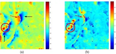
The height difference maps of the created reference DTMs compared to the MSD method (Figure 9a) and the NGPs method (Figure 9b) are both significantly better than the DTMs created for Area 1 (Figure 8). This is mainly due to the fact that the topographic surface is mostly flat, and due to that there are no visible errors in the original DSM. The highlighted area (red circle) in Figure 9a indicates large negative errors from up to 2m in the MSD extracted DTM. The MSD approach is still facing the same challenge as highlighted and discussed previously in Figure 8, and hence confirming previous outcomes. In contrast, the maximum negative error in this area in the DTM created by the NGPs method is smaller by approximately 0.5m. While there are no significant lower sections in the NGPs there is one higher area by nearly 2.5m as shown in Figure 9b. This area is also highlighted previously in Figures 6a and 6b. In fact, the correct value for this area is higher than what our NGPs approach determines. Consequently,
NGPs is significantly better and therefore the DTM values are the closest to the truth values.
Figure 9. Area (2) height differences maps of the created DTMs with LiDAR DTM. MSD (a) and NGPs (b).
Table 4 shows the calculated Mean-squared errors (MSEs) and standard division (SD) of the height differences. The MSE and SD equal to 0.1942 and 0.1079 for DTMs created by MSD, 0.1488 and 0.0873 for (NGPs 4d), and 0.1348 and 0.0879 for (NGPs 8d) respectively. Accordingly, the quality of the created DTM by NGPs is slightly improved in area 2 compared to area 1 due to the fact that area 2 is rather flat. However, similar to area 1, NGPs algorithm requires significantly less time as concluded previously.
MSE SD Computation time MSD 0.1942 0.1079 5480.5 s
NGPs 4d 0.1488 0.0873 319.47 s NGPs 8d 0.1348 0.0879 327.16 s
Table 4. Statistics of mean-square error (MSE) and standard division (SD) of height differences between MSD and NGPs compared with the LiDAR DTM as well as the time required to execute the algorithms.
5. CONCLUSION
This paper presents a simple and powerful filtering algorithm for the DTM extraction from airborne stereo images derived DSMs. This algorithm is an enhancement of the MSD approach proposed by (Perko et al., 2015). In contrast, to the original approach, the newly proposed NGPs approach solves the local slope problem in a more reliable way and with less complexity using reliable and well distributed initial ground points. A further extension is the increase of the number of scanlines. Hence the quality of the generated DTMs and further the nDSMs are significantly improved.
Two different datasets have been used to evaluate the NGPs method, and to compare the performance to the MSD method. In these tests similar filter size for both algorithms were used. The resulting DTMs were evaluated using qualitative and quantitative measurements. The visual inspection, as well as the objective measurements of the mean square error and the standard deviation, confirmed the efficiency and the robustness of the NGPs approach compared to the MSD approach.
However, while the initial DTMs created by our NGPs approach are quite acceptable for certain applications, the introduction of further processing technique maybe required. The goal of those techniques are to simplify and therefore to speed up the processes of the NGPs selection. For instance, it is not necessary to move the filter one by one pixel along the x and y directions over the whole DSM. First experiments show that moving 5 pixels in both directions will very likely yielded similar results but will require less computing time. Furthermore, eliminating very small regions from the created ground regions mask could be a useful option for enhancing the MSE SD Computation time
MSD 0.8560 0.3660 556.06 s NGPs 4d 0.4574 0.2666 50.19 s NGPs 8d 0.3814 0.2492 52.60 s
created DTM accuracy because they might be incorrect (Perko et al., 2015).
In addition, while the inward interpolation technique is so far used for filling holes in the ground mask produces satisfying results, the finally created DTM could be also smoothed by using an average, median, or any other smoothing filter to obtain smoother DTM surfaces.
ACKNOWLEDGEMENTS
This work was supported by The Higher Committee for Education Development (HCED) in Iraq. Thanks to Dr Roland Perko for his cooperation and providing his matlab source code. The Vaihingen data set was provided by the German Society for Photogrammetry, Remote Sensing and Geoinformation (DGPF) [Cramer, 2010]: http://www.ifp.uni-stuttgart.de/dgpf/DKEP-Allg.html.”
REFERENCES
Arefi, H., d'Angelo, P., Mayer, H., & Reinartz, P. 2009. Automatic generation of digital terrain models from cartosat-1 stereo images. Int. Arch. Photogramm. Remote Sens. Spatial Inf. Sci., XXXVIII-1-4-7/W5, pp. 1-6.
Beumier, C., & Idrissa, M. 2016. Digital terrain models derived from digital surface model uniform regions in urban areas. International Journal of Remote Sensing, 37(15), pp. 3477-3493.
Bulatov, D., Häufel, G., Meidow, J., Pohl, M., Solbrig, P., & Wernerus, P. 2014. Context-based automatic reconstruction and texturing of 3D urban terrain for quick-response tasks. ISPRS Journal of Photogrammetry and Remote Sensing, 93, pp. 157-170.
Chaabouni-Chouayakh, H., Arnau, I. R., & Reinartz, P. 2013. Towards automatic 3-D change detection through multi-spectral and digital elevation model information fusion. International Journal of Image and Data Fusion, 4(1), pp. 89-101.
Cramer, M. 2010. The DGPF-test on digital airborne camera evaluation–overview and test design. Photogrammetrie-Fernerkundung-Geoinformation, 2010(2), pp. 73-82.
Förstner, W. 1982. On the geometric precision of digital correlation. Int. Arch. Photogrammetry & Remote Sensing, 24(3), pp. 176-189.
Haralick, R. M., Sternberg, S. R., & Zhuang, X. 1987. Image analysis using mathematical morphology. IEEE transactions on pattern analysis and machine intelligence,(4), pp. 532-550.
Hirschmuller, H. 2008. Stereo processing by semiglobal matching and mutual information. Pattern Analysis and Machine Intelligence, IEEE Transactions on, 30, pp. 328-341.
Krauß, T., Arefi, H., & Reinartz, P. 2011. Evaluation of selected methods for extracting digital terrain models from satellite born digital surface models in urban areas. International Conference on Sensors and Models in Photogrammetry and Remote Sensing (SMPR 2011), pp. 1-7.
Krauß, T., & d’Angelo, P. 2011. Morphological filling of digital elevation models. Proc. ISPRS Int. Arch. Photogramm. Remote Sens. Spat. Inf. Sci. XXXVIII-4/W19, pp. 165-172.
Krauß, T., d’Angelo, P., Kuschk, G., Tian, J., & Partovi, T. 2015. 3D-Information fusion from very high resolution satellite sensors. Int. Arch. Photogramm. Remote Sens. Spatial Inf. Sci., XL-7/W3, pp. 651-656.
Krauß, T., Lehner, M., & Reinartz, P. 2008. Generation of coarse 3D models of urban areas from high resolution stereo satellite images. Int. Arch. Photogramm. Remote Sens. Spatial Inf. Sci., 37, pp. 1091-1098.
Krauß, T., & Reinartz, P. 2010. Urban object detection using a fusion approach of dense urban digital surface models and VHR optical satellite stereo data. Int. Arch. Photogrammetry & Remote Sensing, 39, pp. 1-6.
Meng, X., Currit, N., & Zhao, K. 2010. Ground filtering algorithms for airborne LiDAR data: A review of critical issues. Remote Sensing, 2(3), pp. 833-860.
Meng, X., Wang, L., Silván-Cárdenas, J. L., & Currit, N. 2009. A multi-directional ground filtering algorithm for airborne LIDAR. ISPRS Journal of Photogrammetry and Remote Sensing, 64(1), pp.117-124.
Perko, R., Raggam, H., Gutjahr, K., & Schardt, M. 2015. Advanced DTM generation from very high resolution satellite stereo images. ISPRS Annals of Photogrammetry, Remote Sensing and Spatial Information Sciences, 1, pp.165-172.
Tian, J., Krauss, T., & Reinartz, P. 2014. DTM generation in forest regions from satellite stereo imagery. Int. Arch. Photogramm. Remote Sens. Spatial Inf. Sci.,XL-1, pp. 401-405. The International Archives of the Photogrammetry, Remote Sensing and Spatial Information Sciences, Volume XLII-1/W1, 2017