www.elsevier.nlrlocaterjappgeo
Numerical analysis of 2.5-D true-amplitude diffraction
stack migration
J.C.R. Cruz
), J. Urban, G. Garabito
Received 1 January 2000; accepted 19 May 2000
Abstract
By considering arbitrary source–receiver configurations, compressional primary reflections can be imaged into time or depth-migrated seismic sections so that the migrated wavefield amplitudes are a measure of angle-dependent reflection coefficients. Several migration algorithms were proposed in the recent past based on the Born or Kirchhoff approach. All of them are given in form of a weighted diffraction-stack integral operator that is applied to the input seismic data. The result is a migrated seismic section where at each reflection point the source wavelet is reconstructed with an amplitude proportional to the reflection coefficient at that point. Based on the Kirchhoff approach, we derive the weight function and the diffraction
Ž .
stack integral operator for a two and one-half 2.5-D seismic model and apply it to a set of synthetic seismic data in noisy environment. The result shows the accuracy and stability of the 2.5-D migration method as a tool for obtaining important information about the reflectivity properties of the earth’s subsurface, which is of great interest for amplitude vs. offset
Žangle analysis. We also present a new application of the Double Diffraction Stack DDS inversion method to determine. Ž .
three important parameters along the normal ray path, i.e., the angle and point of emergence at the earth surface, and also the
Ž .
radius of curvature of the hypothetical Normal Incidence Point NIP wave. q2000 Elsevier Science B.V. All rights
reserved.
Keywords: Imaging; Ray; Migration; Inversion
1. Introduction
In the recent years, we have seen an increas-ing interest in true amplitude migration meth-ods. A major part of these works dealt with this
)
Corresponding author. Centro de Geosciencas, Univer-sidade Federal do Para, CP 1611, AV. Bernardo Sayao, 01, 66017-900 Belem-Para, Brazil. Fax:q55-91-211-1693.
Ž .
E-mail addresses: [email protected] J.C.R. Cruz ,
ur-Ž . Ž .
[email protected] J. Urban , [email protected] G. Garabito .
topic either based on the Born approximation as
Ž .
given by Bleistein 1987 and Bleistein et al. Ž1987 , or on the ray theoretical wavefield ap-.
Ž .
proximation as given by Hubral et al. 1991
Ž .
and Schleicher et al. 1993 .
This paper follows the latter alternative of working the migration problem by using the ray theoretical approximation. We consider a geo-physical situation where the propagation veloc-ity of a point-source wave does not vary along
Ž .
one of the three-dimensional 3-D Cartesian coordinate axes, the so-called two and one-half Ž2.5-D model..
0926-9851r00r$ - see front matterq2000 Elsevier Science B.V. All rights reserved. Ž .
Starting from the 3-D weighted modified diffraction stack operator as presented by
Schle-Ž .
icher et al. 1993 , we derive the appropriate method to perform a 2.5-D true-amplitude seis-mic migration. We find the weight function to be applied to the amplitude of the 2.5-D seismic data.
In summary, the paper presents a theoretical development by which we derive an expression for the 2.5-D weight that is a function of ray parameters. We show examples of application of the true-amplitude depth migration algorithm to 2.5-D synthetic seismic data in noisy envi-ronment in order to make the numerical analysis more realistic and to verify the stability and accuracy of the algorithm. In the final part, based on the theoretical development given by
Ž . Ž .
Bleistein 1987 and Tygel et al. 1993 , we
Ž .
apply the Double Diffraction Stack DDS in-version method to determine normal ray param-eters, which are the keys for a more general interval velocity inversion problem.
2. Review of 2.5-D ray theory
2.1. The seismic model
We use the general Cartesian coordinate
sys-Ž .
tem being the position vector xs x, y, z . One
of the main concerns of this paper is to apply the ray field properties to the 2.5-D seismic model in order to study the true-amplitude seis-mic migration method. We think of the earth as a system of isotropic layers, where each layer is
Ž .
constituted by a velocity field ÕsÕ x , whose
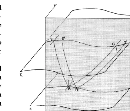
first derivative with respect to the second com-ponent y vanishes in all space. Each layer has smooth surfaces as upper and lower bounds. The upper bound surface So is the earth sur-face. The curvature of each surface is zero along the second component y-axis, i.e., the seismic model has a cylindrical symmetry on
Ž .
the y direction Fig. 1 . The intersection be-tween the plane of symmetry ys0 and the
Fig. 1. 2.5-D seismic model. The in-plane central and paraxial rays start at the earth surface. After reflecting at the reflector, they reach the receiver positions.
earth surface So defines the seismic line. In the 2.5-D seismic model, the wave velocity does not vary along the y direction, while the point-source seismic wave causes 3-D propagation.
At our seismic experiment carried out on So, we consider only P–P primary reflections to be
Ž .
registered at the source–receiver pairs S, G . We assume reproducible point sources with unit strength and receivers with identical character-istics. Their position vectors are denoted by:
xssxs
Ž .
j and xgsxg( )
j ,Ž .
1Ž .
where js j1,j2 is a vector of parameters on
So.
The high frequency primary reflection wave-field trajectory is then described by a ray that starts at the source point S on So, reaches the reflector Sr at the reflection point R, defined
Ž . Ž .
by a vector xrsxr h , hs h1,h2 being a vector of parameters within Sr, and returns to the earth surface at G, the ray path SRG. By considering the 2.5-D case, the ray path SRG is assumed to be totally contained in the plane
ys0.
Ž
the points S and G with components x , x ,1 s 2 s
. Ž .
x3s and x1 g, x2 g, x3 g , respectively. The third coordinate system has its origin at the point R
Ž .
with components x , x , x1r 2 r 3 r . The axes x1 s and x1 g are tangents to the seismic line, while
x3s and x3 g are downward normal to the So.
Ž . Ž .
The components x1r and x3 r are defined in such a way that the former is tangent to the reflector Sr within the symmetry plane ys0, while the latter is upward normal to the reflec-tor. The second components x , x2 s 2 g and x2 r have the same direction as the y component in
Ž .
the general Cartesian coordinate system Fig. 1 .
2.2. Ray theory
The principal component primary reflection of the seismic wavefield generated by a com-pressional point source located at x and regis-s
tered at xg is expressed in the 3-D zero-order
Ž .
ray approximation given by Cerveny 1987 as:
´
U
Ž
j,t.
sU W toŽ
ytŽ .
j.
.Ž .
2The above cited principal component primary reflection describes the particle displacement into direction of the ray at the receiver point G.
Ž . Ž .
In Eq. 2 , W t represents the analytic point-source wavelet, i.e., this is a complex valued function whose imaginary part is the Hilbert transform of the real source wavelet, and the real part is the wavelet itself. At the receiver position xg within the surface So, the seismic trace is the superposition of the principal com-ponent primary reflections.
Ž . The reflection traveltime function tst x
satisfies the 3-D eikonal equation
=tP=ts1rÕ2
Ž .
x ,Ž .
3Ž .
Being ÕsÕ x the P wave velocity. The
am-plitude factor U can be expressed by:o
U sUÕ=t,
Ž .
4o o
Ž .
where UosU x is a scalar function that satis-o fies the 3-D transport equation, in constant den-sity and varying velocity media, given by:
2
Ž
=tP=U.
Õ2Ž .
x qÕ2U=2tqUŽ
=tP=Õ2.
o o o
s0.
Ž .
5By considering only the 2.5-D wave propaga-tion within the symmetry plane ys0, that is of interest, we assume j2sh2s0, j1sj and
h1sh, simplifying the notation, so that we
Ž . Ž . Ž .
have xssxs j , xgsxg j and xrsxr h .
Ž .
Following Bleistein 1986 , we introduce the fundamental in-plane slownessÕector:
t
ps
Ž
p, q.
s s=tŽ
x , z ,.
Ž .
6Õ
Ž
x , z.
where the two-components unitary vector t is Ž . tangent to the in-plane ray trajectory. In Eq. 6 , the components p and q are the so-called hori-zontal and vertical slowness, respectively, which are related to each other by the expression:
1 2
qs"
(
Õ2yp .Ž .
7By using the in-plane initial values of the
Ž .
where b and Õ are the start angle of the ray
o o
Applying the above in-plane ray equations, Ž . and considering the initial conditions 8 , to the
Ž . fundamental solution of the transport Eq. 5 as
Ž .
found in Cerveny 1987 , the amplitude factor
´
of the in-plane reflected wavefield is computed by:In formula 13 , R is the geometrical-opticsc reflection coefficient at the reflection point R as
Ž .
presented by Bleistein 1984 . The factor AA
corresponds to the total lost energy due to the transmission across all interfaces along the whole ray. In general, we assume this factor to be negligible, i.e., the transmission loss to be very small, or to be corrected by other means. The amplitude factor LL2.5 is called in-plane
point-source divergence factor or geometrical
spreading, whose expression will be given in
the Section 2.3.
2.3. Paraxial ray approximation
The paraxial ray approximation is based on the a priori knowledge of a ray trajectory also known as the central ray, which in our example
Ž .
is the ray that starts at the source S j , reaches Ž . the reflector at the reflection point R h , and
Ž .
arrives at the receiver G j . Thus, a paraxial
ray is any ray that starts in the vicinity of S, at
XŽ X. XŽ X.
the point S j , reflects at the point R h
nearby the point R, and reaches the receiver
X
Ž X
. Ž .
point G j in the vicinity of G Fig. 1 . By applying the concept of paraxial rays,
Ž .
Cerveny
´
1987 derived the paraxial eikonal equation having as solution the two-point parax-ial reflection traveltime from point SX at xXssŽ X. X X Ž X.
xs j to the point G at xgsxg j in the vicinity of points S and G, respectively. An equivalent second-order approximation solution
Ž .
was found also by Ursin 1982 and Bortfeld Ž1989 . In this paper, we use the formalism of.
Ž .
Schleicher et al. 1993 tailored to the in-plane
ray trajectory. The reflection traveltime is then given by: denotes the traveltime along the central ray SG, while s and g are linear distances in the axes
x1 s and x1 g, the so-called paraxial distances. Ž . These distances are obtained as follows: 1 At the source–receiver points SX and GX, the vec-tors xXs and xXg are orthogonally projected onto
Ž .
the respective axis x1 s and x1 g; 2 the dis-tances s and g are then defined as having origin at the source–receiver points S and G with end at the extremity of the projections of
xXs and xXg, respectively. On the other hand, the so-called local horizontal slowness p and pS G
are obtained by two cascaded orthogonal projec-tions of the initial and final in-plane slowness vectors at source–receiver points SXand GX onto the respective axes x1 s and x1 g.
The quantities NG and NS are
second-de-S G
Ž . rivatives of the traveltime function 14 with respect to the source and receiver coordinates evaluated at ss0 and gs0, respectively. The other quantity NSG is the second-order mixed-Ž . derivative of the same traveltime function 14 evaluated at ssgs0.
In the next section, we will perform the 2.5-D true-amplitude migration by using a proper weighted modified diffraction stack. For that, we define for all points of parameters j on the earth surface, and each point M within a specified volume of the macro-velocity model, the diffraction in-plane traveltime curve:
tD
Ž .
j stŽ
S, M.
qtŽ
M ,G.
stSqtG.Ž .
15Ž .
Following Schleicher et al. 1993 , we will refer to this curve as the Huygens traÕeltime.
arbitrary point M within the model, and from
M to the receiver point G.
For obtaining the Huygens paraxial travel-time at a reflection point within Sr in the
Ž . X
two equations of type 14 for the paraxial traveltime from SX to RX
In both formulas 16 and 17 , the quantity r is the linear distance between R and the extrem-ity of the orthogonal projection of xXr onto the axis x1r tangent to the reflector at the point R. The local horizontal slowness p is built by twor
cascaded projections of the in-plane slowness vector at x onto the xr 1 r axis.
It is necessary to point out that in general, the earth surface is not a horizontal plane, instead, it can be even an arbitrary surface. In our case, we consider it as a smooth surface with cylindrical geometry with axis in direction of the y coordi-nate. Thus, s and g are paraxial distances eval-uated within tangent planes to the earth surface
Ž X
. at S and G, respectively. Moreover, x xs s and
Ž X. Ž X.
xg xg are position vectors of the points S S Ž X
.
and G G in the general Cartesian coordinates. The same geometrical assumption is required for the reflector surface, by the way the paraxial distance r is evaluated within the tangent plane
Ž X
.
at the reflection point, while xr xr are the Ž X
. position vectors of the points R R .
The quantities NSR and NRG are second-order mixed-derivatives, respectively of the
travel-Ž . Ž .
times 16 and 17 calculated at ssgsrs0,
while NSR and NRS are the second-order deriva-Ž .
tives of the traveltime function 16 with respect to s and r, respectively. The quantities NG and
R
NGR are the second-order derivatives of the trav-Ž .
eltime function 17 with respect to r and g.
Ž . Ž .
Following Bleistein 1986 , Liner 1991 ,
Ž . Ž .
Stockwell 1995 and Hanitzsch 1997 , the ex-pression of the geometrical spreading factor, when tailored to the 2.5-D zero-order ray ap-proximation of the seismic wavefield, is given by:
and aG are the start and emergence angles of the central ray measured with respect to the normal at S and G on the earth surface, while
Õ is the velocity at the source point S. The term
s
N
N in the denominator is given by the ratio:
NSRNGR quantities related with each branch of the in-plane central ray SR and RG, and calculated by the expressions:
The exponential term in Eq. 18 represents the phase shift due to the caustics along each branch of the central ray. For obtaining this factor, it is necessary to use dynamic ray trac-ing.
Ž .
From Eq. 18 , the 2.5-D geometrical spread-ing LL can be expressed then as function of
2.5
the 2-D spreading LL2, given by:
L
L2.5sLL F2F2.5, FF2.5s
(
sSqsG,Ž .
21 where FF is called the out-of-plane factor.2.5
parame-ters of 2-D rays. The 2.5-D amplitude factor of the zero-order ray approximation is then rewrit-ten as:
denotes the in-plane 2-D wavefield amplitude. An equivalent relationship between 2-D and 2.5-D amplitude factors can be found in
Bleis-Ž .
tein 1986 . This means that if we know the 2-D amplitude factor, we need only to divide it by the out-of-plane factor FF in order to obtain
2.5 the 2.5-D amplitude.
3. 2.5-D ray migration theory
By following the zero-order ray approxima-tion of the 2.5-D seismic wave, we have the true-amplitude defined as:
UTA
Ž .
t sLL2.5Ž
Uo. Ž
2 .5 j,tqtR.
sR W t .cŽ .
23Ž .
In order to build the appropriate true-ampli-tude migration operator, we start from the 3-D
Ž .
integral given by Schleicher et al. 1993 :
y1
where the symbol P means the first derivative
Ž .
with respect to time, and w j, M is the weight function used to stack.
By assuming the paraxial distances s and g to be linear functions of j, we can write:
ssG jS and gsG jG ,
Ž .
25Ž . Ž .
where GSs EsrEj and GGs EgrEj , which are calculated at js0. In the same way, we consider r a linear function of h so that:
Er
rsG hr , where Grs .
Ž .
26Eh
Ž . As a consequence of the above relations 25
Ž .
and 26 , we can express the traveltime
func-Ž . Ž .
By using the result obtained in the Appendix
Ž .
by Eq. A8 , we have the 2.5-D modified diffraction stack integral in frequency domain given by the stationary phase solution:
'
yivˆ
ˆ
V R ,
Ž
v.
fH
djw2.5Ž
j, R U.
2.5Ž
j,v.
'
2p A=exp ivtD
Ž
j, R.
.Ž .
27 Inserting the 2.5-D zero-order approximation Ž13 of the primary reflection into integral 27. Ž . we have:The above integral 28 is once again calcu-lated approximately by the stationary phase method. At this time, we apply the stationary
After some algebraic manipulations involving
Ž . Ž . Ž .
the 14 , 16 and 17 , we can express the second-order derivative term by:
2
The 2.5-D weight function at an arbitrary point M in the macro-velocity model through the high frequency approximation of the diffrac-tion stack integral, for a critical point j)
within the migration apperture A. The weight function is then obtained so that the stack integral is asymptotically equal to the spectrum of the true-amplitude migrated source wavelet multi-plied by a phase shift operator. In other words, the phase of the asymptotical result is shifted by a quantity equal to the difference between the in-plane reflection and diffraction traveltime curves at the stationary point. Thus, we have:
ˆ w ) x )
By using the stationary phase approximation Ž29 and definition 32 , the 2.5-D weight func-. Ž . tion is then obtained as:
w j)
After replacing the appropriate definition of Ž .
L
L as given by Eq. 18 and including the
2.5
Y
Ž . evaluation of tF from the expression 31 , we have the result:
Based on the 3-D weight function found in
Ž .
Tygel et al. 1996 by using the so-called
Ž .
Beylkin’s determinant, Martins et al. 1997
Ž )
. derived a similar 2.5-D weight wJ j , M . This result is related with the 2.5-D weight function given in the present paper by:
yip
The difference between both results can be explained by the assumption used in Beylkin
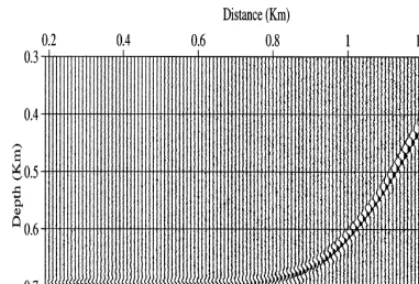
Fig. 3. 2.5-D true-amplitude depth migrated seismic data, real part, obtained after migrating the synthetic seismic data in Fig. 1.
Ž1985 , which does not allow for any caustics. along rays.
The above weight function is to be applied to the amplitude of the 2.5-D seismic data, that is generated when we have a situation of a point source lined up to a set of receivers in the plane
j2s0, by considering a seismic model where the velocity field does not depend on the second coordinate j2. If the chosen point M inside the model coincides with a real reflection point R and jsj)
, the result of applying the difraction
Ž Ž ..
stack migration operator Eq. 28 to the seis-mic data is proportional to the reflection coeffi-cient. Putting this result into the point R, we have the so-called true-amplitude depth mi-grated reflection data. In cases of special con-figurations, we can apply the weight function Ž34 as follows: 1 Common-offset:. Ž . GGsGSs
Ž .
1 for S/G; 2 Common-shot: GSs0 and Ž .
GGs1 when the source point S is fixed; 3
Common-receiver: GSs1 and GGs0 when the Ž .
receiver point G is fixed; and 4 Zero-offset:
GSsGGs1 for S'G, and then aSsaG, k1 sk2 and sSssG. In the common-midpoint configuration, the weight function is not ade-quate because in this case, the stationary phase solution is not valid.
4. Application of 2.5-D true-amplitude migra-tion
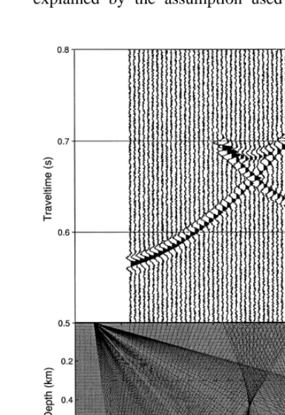
The true-amplitude migration algorithm was tested on synthetic data obtained from the SEIS88 ray tracing software. The seismic model is constituted by a layer above an arbitrary
Ž .
curved reflector Fig. 2 . The interval velocity of the P–P wave in the overburden is 2.5 kmrs, and 3.0 kmrs in the half-space. The seismic data was generated into a common-shot configuration, with the source at xs0.1 km in the earth surface and 177 geophones positioned between 0.3 and 1.4 km, being the geophone interval distance 6.25 m. The source pulse is represented by a Gabor wavelet as proposed by
Ž .
Gabor 1946 , with frequency 80 Hz, while the seismic trace has the sample interval of 0.5 ms. In the seismic data a random noise with uniform distribution was added, in which the maximum value is 10% of the maximum amplitude of the seismic data. The macro-velocity model and the seismogram with noise are presented in Fig. 2. The seismic data were migrated by using the true constant velocity model, having the target zone 0.19FxF1.32 km; 0.3FzF0.75 km, with Dxs5 m and Dzs1 m. The migrated
Ž .
seismic image real part is presented in Fig. 3. In Fig. 4, we have the reflection coefficients, where the continuous line corresponds to the exact values, while the crosses indicate the am-plitudes determined from the migrated section. As a consequence of the addition of noise to the input data, the seismic migration algorithm does not correctly recover the original source wavelet. But even in spite of the noise, we can see that the obtained seismic image represents the true
reflector very well. In case of noise in the data, it is not so easy to determine where the so-called boundary effects begin to influence the migrated data.
5. Seismic inversion method
Based on the Born and on the ray theoretical
Ž .
approximations, Bleistein 1987 and Tygel et
Ž .
al. 1993 , respectively, presented a new inver-sion method, the so-called DDS, through which it is possible to estimate several parameters on the trajectory of a selected ray between the source and geophone, for any arbitrary configu-ration of the seismic data. This inversion tech-nique is based on the weighted diffraction stack migration integral, used above for determining the reflection coefficient. In this paper, the DDS inversion technique is used to determine three
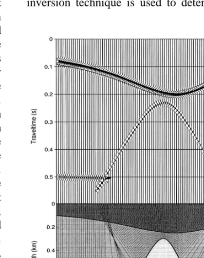
Fig. 5. Synthetic seismic data, used as input in the DDS inversion technique. The seismic model is constituted by two layers above a half-space, with velocities 2500 mrs
parameters related to the trajectory of the nor-Ž .
mal reflection ray, to be known: 1 the radius of curvature, RNIP, of the Normal Incidence
Ž .
Point NIP wave associated with the normal Ž .
ray; 2 the emergence point xo of the normal Ž .
reflection ray; and 3 the emergence angle bo
of the normal reflection ray. The NIP wave, as
Ž .
defined by Hubral 1983 , is a hypothetical
wave that starts at the reflection point at time zero, propagates with half the medium velocity and returns to the earth surface at the two-way time of the normal ray.
By applying the DDS inversion technique, we make use of the weighted diffraction stack
Ž .
integral. Alternatively, we write V M,t s
Ž .
V M,t , where j is the index for specifying thej
Ž .
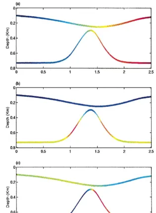
Fig. 6. Final products of the DDS inversion technique: a coordinate of the emergence points of the normal reflection rays;
Ž .
Fig. 7. Exact values of wavefront parameters calculated by ray theory: a coordinate of the emergence points of the normal
Ž . Ž .
reflection rays; b radii of curvatures of the NIP waves; c emergence angles of the normal reflection rays.
used weight to stack the input data. The DDS inversion technique is then done by a double stack, each one with a different weight function
js1 and js2. The result is obtained by the ratio between the two stacks given by:
V M ,t1
Ž
.
VDDS
Ž
M ,t.
s .Ž .
36V2
Ž
M ,t.
If we choose as the weight function for the first stack a ray parameter specified by the trajectory starting at point M in the reflection point up to the earth surface, and for the second stack the unity, the VDDS will result in the value of the selected ray parameter. In this paper, we have used for the first stack the values of RNIP,
subsurface, having as input data a zero-offset seismic section. The result of this inversion technique is a mapping of normal ray parame-ters associated with primary reflection events in the zero-offset data. By choosing a minimum amplitude value in the denominator of the
for-Ž .
mula 36 , we have empirically avoided the division by zero in the DDS algorithm.
6. Application of the DDS
In order to do a numerical experiment, we have generated a set of zero-offset seismic traces by using the ray theoretical modeling algorithm SEIS88. We have used the seismic model of Fig. 5 constituted by two layers above a half-space with two reflectors. The P–P wave ve-locities are 2500 and 3000 mrs for the first Župper. and second Žbottom. layers, respec-tively. By using a Gabor wavelet as proposed
Ž .
by Gabor 1946 with a frequency of 60 Hz, a sample interval of Dts1 ms and a space inter-val Dxs25 m, we have obtained an ensemble
Ž .
of zero-offset seismograms Fig. 5 used as input data in the DDS process. The final prod-ucts are obtained by using the same P-wave velocities of the original seismic model, in order to find the following parameters of the normal
Ž .
rays at the second interface: 1 the coordinates of the emergence points of the reflection normal
Ž . Ž .
rays Fig. 6a ; 2 the radii of curvatures Žradiusgram of the NIP waves associated with.
Ž . Ž .
each reflection normal ray Fig. 6b ; and 3 the emergence angles of the reflection normal rays Žanglegram. ŽFig. 6c . As we can see in Fig. 7a,. b and c, the obtained values by DDS technique are very similar to the true values, which vides an evaluation of the accuracy of the pro-posed inversion method.
In the above results, we have shown that the DDS inversion technique can be used for deter-mining a selected parameter along the ray tra-jectory. The three parameters here obtained ŽRNIP, bo, xo. are the key for solving the interval velocity inversion problem. A more
de-tailed discussion about the inverse problem can
Ž .
be found in Hubral and Krey 1980 .
7. Conclusion
Starting from the paraxial ray theory, we have derived a 2.5-D weight function to be used in the 2.5-D diffraction stack migration opera-tor. Based on the double diffraction stack inver-sion technique, we have also built an algorithm to determine fundamental parameters related to the normal ray trajectory. From the results ob-tained in this paper, we claim that the present 2.5-D weight function when applied to the 2.5-D seismic data is able to recover the reflection coefficient even in a noisy environment. The 2.5-D true-amplitude migration algorithm is sta-ble, i.e., we have that small perturbation in the input data provides only slight deviation in the output migrated data. It is to be stressed that the proposed 2.5-D true-amplitude migration algo-rithm works very good in more complex situa-tions when there are triplicasitua-tions in the input data due the presence of caustics. In addition, we have shown that the DDS inversion tech-nique is able to determine parameters along the ray trajectory that are of interest for the interval velocity inversion problem.
Acknowledgements
Appendix A
Ž .
Following Schleicher et al. 1993 , the weighted modified diffraction stack is consid-ered an appropriate method to perform a true-amplitude migration. For each point M in the
Ž .
macro-velocity model and all points j1,j2 in the migration aperture A, the diffraction stacks are then performed by summation along the
Ž .
Huygens surfacestD j1,j2, M for all points M into a region of the model. The true-amplitude migration is achieved by the summation using certainly Huygens surface and derived weight function, such that the stack output is propor-tional to the desired reflection coefficient. Mathematically, this operation is described by the 2-D integral
where the symbol P means the first derivative
Ž .
with respect to time, and w j, M is the weight function used to stack.
Ž .
By transforming the expression A1 into the frequency domain:
In order to specialize the 3-D formula A2 to the 2.5-D geometry, we start considering Ms
R, i.e., the reflection point itself. The migration
integral needs to be solved asymptotically by the stationary phase method as found in
Bleis-Ž .
tein 1984 with respect to the coordinate j2, by making use of the stationary condition as showed
Ž .
in Bleistein et al. 1987 :
EtD Et
Ž
SŽ .
j , R.
EtŽ
R ,GŽ .
j.
s q N sSo 0,
Ej2 Ej2 Ej2
A3
Ž
.
which can be expressed through the identity:
E
< <
t
Ž
S, M.
qtŽ
M ,G.
Sosp2 sqp2 g So Ej2s0.
Ž
A4.
By applying the in-plane ray condition p2s
p2o into the 3-D ray equation as given by
Ž .
Cerveny 1987 , we have:
´
x2 ssssp2 sNSoand x2 gssgp2 gNSo,
Ž
A5.
with ss and sg calculated along the ray pathsSM and MG, respectively. By considering the
2.5-D geometry, x2 ssx2 gsj2, we finally have
From Eq. A6 , we conclude that the station-ary phase condition is j2s0. For completeness of our asymptotic analysis, we calculate the second derivative of the phase at j2s0
E2 1 1
Here, so and so are the ray parameters for
S G
the ray branches RS and RG, calculated on the earth surface So.
The above results yield the stationary phase solution the in-plane observed point-source wavefield amplitude factor, the 2.5-D weight function is defined as:
y1r2 1 1
w2.5
Ž
j, R.
swŽ
j, R.
ž
soqso/
,Ž
A9.
Ž .
where w j, R is the in-plane version of the 3-D weight function of the 3-D modified diffraction
Ž .
stack by Schleicher et al. 1993 . The weight
Ž .
expression A9 can be readily generalized to any arbitrary depth point M.
References
Beylkin, G., 1985. Imaging of discontinuities in the in-verse scattering problem by inversion of a causal gener-alized radon transform. J. Math. Phys. 26, 99–108. Bleistein, N., 1984. Mathematics of Wave Phenomena.
Academic Press.
Bleistein, N., 1986. Two-and-one-half dimensional in-plane wave propagation. Geophys. Prospect. 34, 686–703. Bleistein, N., 1987. On the imaging of reflectors in the
earth. Geophysics 52, 931–942.
Bleistein, N., Cohen, J.K., Hagin, F.G., 1987. Two and one-half dimensional Born inversion with an arbitrary reference. Geophysics 52, 26–36.
Bortfeld, R., 1989. Geometrical ray theory: rays and
travel-Ž
times in seismic systems second-order approximation
.
of the traveltimes . Geophysics 54, 342–349.
Cerveny, V., 1987. Ray Methods for Three-dimensional´
Seismic Modeling. Norwegian Institute for Technology. Gabor, D., 1946. Theory of communication. J. IEEE 93,
429–441.
Hanitzsch, C., 1997. Comparison of weights in prestack amplitude-preserveing Kirchhoff depth migration. Geo-physics 62, 1812–1816.
Hubral, P., 1983. Computing true amplitude reflections in laterally inhomogeneous earth. Geophysics 48, 1051– 1062.
Hubral, P., Krey, T., 1980. Interval Velocities from Seis-mic Reflection Time Measurements. SEG.
Hubral, P., Tygel, M., Zien, H., 1991. Three-dimensional true-amplitude zero-offset migration. Geophysics 56, 18–26.
Liner, C., 1991. Theory of a 2.5-D acoustic wave equation for constant density media. Geophysics 56, 2114–2117. Martins, J.L., Schleicher, J., Tygel, M., Santos, L.T., 1997. 2.5-D true-amplitude migration and demigration. J. Seism. Explor. 6, 159–180.
Schleicher, J., Tygel, M., Hubral, P., 1993. 3-D true-ampli-tude finite-offset migration. Geophysics 58, 1112–1126. Stockwell, J.W., 1995. 2.5-D wave equations and
high-frequency asymptotics. Geophysics 60, 556–562. Tygel, M., Schleicher, J., Hubral, P., Hanitzsch, C., 1993.
Multiple weights in diffraction stack migration. Geo-physics 57, 1054–1063.
Tygel, M., Schleicher, J., Hubral, P., 1996. A unified approach to 3-D seismic reflection imaging: Part 2.
Ž .
Theory. Geophysics 61 3 , 759–775.