Multi-objective particle swarm optimization for repairing inconsistent comparison matrices - Binus e-Thesis

(1)

International Journal of Computers and Applications, Vol. 36, No. 3, 2014

MULTI-OBJECTIVE PARTICLE SWARM

OPTIMIZATION FOR REPAIRING

INCONSISTENT COMPARISON MATRICES

Abba Suganda Girsang,

∗

_{Chun-Wei Tsai,}

∗∗

_{and Chu-Sing Yang}

∗

Abstract

To repair an inconsistent comparison matrix, two objectives should be minimized, namely the deviation between the original matrix and the modified matrix and the consistency ratio of the modified matrix. However, there will be a conflict if an attempt is made to optimize them together when repairing the inconsistent matrix. This paper proposes a method that uses particle swarm optimization to optimize both objectives when repairing an inconsistent comparison matrix. Some examples of inconsistent matrices are repaired using the proposed method. The results show that the proposed method produces good alternative solutions that satisfy both objectives when repairing inconsistent matrices.

Key Words

Particle swarm optimization, inconsistent matrix, multi-objective optimization, consistency ratio

1. Introduction

In multi-criteria decision problems, decision makers (DMs) construct a set comparison of decision alternatives pre-sented as a comparison matrix [1]–[7]. An important issue for comparison matrices is consistency. The degree of ma-trix consistency represents the logical respondent opinion. An inconsistent comparison matrix cannot be used to make decisions. The consistency of comparison matrices has been extensively studied. Saaty defined consistency using a threshold of consistency ratio (CR, see (1) and (2)) of 0.1. Many methods for repairing inconsistent comparison matrices have been proposed [8]–[17]. There are two con-siderations when modifying an inconsistent matrix. The first consideration is minimizing the deviation between the original and the modified comparison matrices. A mini-mal deviation preserves the original judgment of the DMs.

∗_{Department of Electrical Engineering, Institute of Computer}

and Communication Engineering, National Cheng Kung Uni-versity, Tainan, Taiwan; e-mail: [email protected], [email protected]

∗∗_{Department of Computer Science and Information Engineering,}

National Ilan University, Yilan, Taiwan; e-mail: cwtsai0807@ gmail.com

Recommended by Dr. M. Hamza

(DOI: 10.2316/Journal.202.2014.3.202-3940)

Ma [12] proposed two variables of deviation (δ and σ) to demonstrate the diﬀerence between the original and the modified matrices. They suggested thatδandσshould be less than 2 and 1, respectively. Lin et al. [13] and Yang et al. [14] proposed a diﬀerence index (Di) to determine the deviation between the two matrices. The second con-sideration is minimizing CR. A consistent matrix denotes the logic of judgement of DMs. ACRof 0 indicates perfect consistency. Erguet al. [11] proposed the induced matrix to find the elements that lead to an inconsistent matrix.

1.1 Motivation and Contribution

Ideally, the deviation between the two matrices and the CR should be minimized when repairing an inconsis-tent comparison matrix. However, these objectives are conflicting; that is, a high CR generally leads to low deviation, and vice versa. There is thus no single best solution to such a problem [8], [15]–[17]. Multi-objective optimization is considered an appropriate method for solving this problem. Metaheuristic algorithms are applied to multi-objective optimization in a wide variety of problems. Particle swarm optimization (PSO) is widely used for single-objective optimization due to its high speed of convergence [18]. The performance on single-objective optimization has motivated researchers to use this swarm intelligence to solve multi-objective optimization problems [19]–[23].

However, according to the best of our knowledge, until now, multi-objective optimization has not been applied for repairing inconsistent comparison matrices. Therefore, this study applies PSO to minimize both deviation and CR. The variable Di is used to denote deviation. The thresholdsδandσare set to less than 2 and 1, respectively, as suggested by Ma [12]. Many consistent comparison matrices are given as solutions for repairing an inconsistent matrix. The collections of the node solutions that are set from two objectives are shown in a Pareto graph.

1.2 Organization

(2)

the diﬀerent indexes, as well as the problem definition. Section 3 provides a detailed description of the proposed algorithm. A performance evaluation of the proposed algorithm is presented in Section 4. Conclusions are given in Section 5.

2. Related Work 2.1 Consistent Ratio

The analytic hierarchy process (AHP) is a decision-making tool for organizing and analysing complex decisions. In the AHP, a comparison matrix is used to represent the judg-ment of DMs. An elejudg-ment in a comparison matrix reflects a subjective opinion that indicates the strength of a pref-erence or feeling [24]. Saaty [1] proposed a nine-value scale (1,2,3, . . . ,9) to define the elements of a comparison ma-trix. The elements are denoted as aij, which defines the

dominance of alternative i over j, where 1< aij<9, and

aij= 1/aji. The consistency of a comparison matrix must

be confirmed to verify the logical respondent opinion. An inconsistent matrix cannot be used for decision-making. Saaty [25] defined consistency as the intensities of relations among ideas or objects based on a particular criterion in which they justify each other in some logical way. The consistency rate can be measured in more than two criteria (n >2). If there is only one criterion, there can be no comparison. Thus, a consistent judgment is not needed. If there are only two criteria, the judgment of the DM should be always consistent. Saaty [1] proposed a method for measuring CR, which is defined as (1) and (2). CI is the consistency index, n is the number of criteria or matrix size, andRI is the random consistency index (the average index of randomly generated weights, which must vary according to each matrix order):

CI = (λmax−n)/(n−1), forn >2 (1)

CR =CI/RI, forn >2 (2)

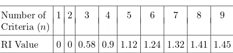
RI values for various matrix sizes are shown in Table 1. Due to the fact that n must be larger than 2, RI will never be 0. Matrices with a CR value of less than 0.1 are consistent. Perfect consistency is obtained when the eigenvalue maximum equals the number of criteria (λmax=n).

Table 1

RI Values for Various Matrix Sizes

Number of 1 2 3 4 5 6 7 8 9

Criteria (n)

RI Value 0 0 0.58 0.9 1.12 1.24 1.32 1.41 1.45

2.2 Diﬀerence Index

Ideally, the modified matrix is cultivated to be closer to the original matrix. By chasing the closer original matrix, it will maintain the original decision. There are several

methods to measure the distance between the two matrices. In this study, the Di is used to measure the distance between the two matrices. The reason Di is preferred in this study, as Lin et al. [13] mentioned, is because using theDi reflects more real diﬀerence between the same gene values in two genotypes. Di is defined as described in (3):

Di=

₍_G_′_/G_{) + (}_G/G_′₎

n2₋₁ −1 (3)

whereG′ _and_G_{are row vectors comprising the lower} tri-angular elements of the substitute matrix A′ _{and of the} original matrixA, respectively; “/” refers to the element-to-element divisions. A smallerDi indicates more similar-ity between two matrices. Di will be 0 if the two matrices are identical.

2.3 Problem Definition

The CR and the diﬀerence index should be minimized when modifying a comparison matrix. For a consistent matrix, the thresholdCRmust be less than 0.1. Therefore:

MinF1=CR

0< F1<0.1

(4)

The deviation between the original matrix and the modified matrix should be minimized:

MinF2= (Di) (5)

Besides these two objectives, the two variables of deviation (δ and σ) proposed by Ma [12] are used as additional constraints. The thresholdsδandσshould be less than 2 and 1, respectively. δandσare, respectively, denoted as:

δ = max

In PSO, each particle moves in the search space trying to get the best position. The position is aﬀected by a particle’s historically best position (local best) and the swarm’s best position (global best). To implement the position in PSO, the particle position of an element in a matrix can be encoded from the lower triangular comparison matrix. The element matrix (aij) is related to its transpose (aji), that

is,aij= 1/aji. Figure 1(a) shows a sample matrixAwhose

(3)

Figure 1. (a) Matrix A with n= 4 and (b) encoding of matrixA.

by sequentially picking elements of the lower triangular matrix A, which is represented as GA in Fig. 1(b), row

by row.

The number of elements ofGAis (n2−n)/2. If matrix

Ais identified as an inconsistent matrix and requires repair, then the scale value of the sequence nodes should be given new values. As previously mentioned, there is no one optimal solution. Non-dominated solutions are constructed by the relation Di and CR. To generate them, there are three steps in which each step uses PSO to obtain the result matrices.

1.Minimize Di. The first step is to modify the matrix such that the Di is minimized. The optimal Di is performed to obtain the consistent matrix, yet main-tains the modified judgment that is closer to the origi-nal DM judgment.

2.Minimize CR. The second step is to modify the matrix such that theCR is minimized.

3.Obtain set of non-dominated solutions. The third step is to find the set nodes CR–Di by iteratively decreasing the thresholdCR. In the beginning, the op-timalDi is determined using the threshold maximum CR (CR<0.1). After the optimal Di is obtained with a CR<0.1, the CR is decreased, and CR−k

is produced to obtain the next Di. This process is repeated until the minimalCR obtained in the second step is achieved.

All the steps have the following constraints: (a)CR<0.1, (b) δ <2, and (c) σ <1. Constraint (a) guarantees a consistent matrix. Constraints (b) and (c) guarantee that the transformation of the original values is acceptable.

3.2 The Proposed Algorithm

Generally in PSO, a particleistarts moving with a velocity

Vi(t+1)from its current position,Xi(t), to the next position,

Xi(t+1), as in (8). The velocity is influenced by three

factors: (a) previous velocity, Vi(t), (b) the best previous

particle position, Xp(t), and (c) the best previous swarm

particle position,Xg(t). It can be stated as (9):

Xi(t+1) = Xi(t)+Vi(t+1) (8)

Vi(t+1) = (w∗Vi(t)) + (C1∗R1(Xp(t)−Xi(t))

+ (C2∗R2(Xg(t)−Xi(t))) (9)

where w is the weight to control the convergence of the velocity, C1 is the acceleration weight cognitive element,

C2 is the weight of social parameter, and R1 and R2 are random numbers in the range [0,1].

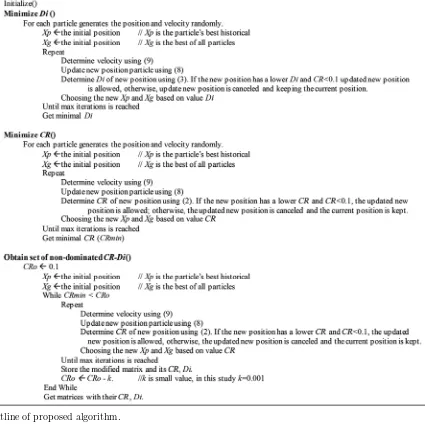
As mentioned in the concept above, this proposed method involves three important steps in which each step uses PSO to obtain the modified the comparison matrix. The first, second, and third step are intended to find the minimalDi,CR, and non-dominatedCR–Di, respectively. The first two steps use the origin PSO, yet the third step uses a modified PSO. This modified PSO actually uses the original PSO (like the second step), but adds a performing reiteration with a new boundaryCR(CRo) to obtain some new values forCR–Di. These steps are shown in Fig. 2.

In the minimize Di _{step, firstly, the each particle} (there are 300 particles) generates its position and its velocity randomly. The position particle means that the particle generates randomly the candidate for the modified matrix. The element matrix can be represented only by the lower triangular matrix elements consecutively. The velocity particle means that the particle generates the value as adding/diminishing the position of the particles. Due to the scale value of positions 0.111–9, the initial value velocity is not high. We take the value position to be limited below 0.1. The best historical particle is defined as Xp, and the best position for all particles is defined asXg. Initially,Xpis taken from the first position particle generated, whileXgis taken from the best position from the first position of all particles generated. In next iteration, based on the previous velocity information, Xp, Xg, and some variables (w, C1, C2, R1, R2), the velocity of each particle is updated, as described in (9). To set the value of variables, some experiments are conducted. The new position will be obtained based on the updated velocity, as described in (8). Due to minimizing Di, the evaluation of the fitness function uses Min F2(Di), as described in (5). However, if a particle’sDi is worse than before, or theCR>0.1, the update will be cancelled. Also, the result of this fitness function also updates the new best historical position of each particle (Xp) and the new best position of all particles as a group (Xg). This process is repeated until the iteration maximum is reached.

The process to minimizeCR _{is almost same as the} process to minimizeDi. If the process to minimizeDi uses the MinF2(Di) as its fitness function, then the process to minimizeCR uses MinF1(CR), which is described in (3) as its fitness function.

The process toobtain set of non-dominated CR_– Di _{solutions is also same as the process to minimize} Di. Yet, the process adds some various CRs, which are decreased gradually untilCRmin is reached.

3.3 Determining the Pareto Graph

A Pareto graph is built using the solution nodes. Initially, archive A is empty, and all of the solution nodes are candidates (C). The nodes chosen as solutions are added to archiveA. Not every node inC is added toA. Figure 3 depicts the process for how to select a candidate C to archiveA.

(4)

Figure 2. Outline of proposed algorithm.

Figure 3. Three conditions for selecting an archive candidate.

(b) IfC is dominated by at least one member in A, then

Cis not put inA(Fig. 3(b)).

(c) If neitherCnorAdominate each other, thenCis put inA(Fig. 3(c)).

4. Experimental Results

This section evaluates the proposed method by applying it to some comparison matrices. The proposed method is also compared to an existing method.

4.1 Parameter Setting and Dataset Matrix

The method proposed in this study consists of three steps. All of them use the following settings: w= 0.1; C1= 0.2;

C2= 0.3; R1= 0.4; andR2= 0.5. The numbers of swarms and iterations are set at 300 and 100, respectively. The dataset matrices are shown in Table 2, some of which are

Table 2

Inconsistent Matrices Used for Evaluation

Matrix Value CR

Size 3×3

M1 5; 5-0.2a 0.254

M2 5; 0.333-0.2a 0.117

Size 4×4

M3 9; 0.333-0.2; 5-0.5-2b 0.172

M4 0.2; 3-5; 0.25-0.5-0.5c 0.191

Size 5×5

M5 3; 0.5-0.143; 6-9-9; 2-4-4-0.2 0.139

M6 0.333; 0.111-2; 1-7-8; 2-0.5-7-0.5 0.307 Size 6×6

M7 0.5; 9-3; 1-4-0.2; 5-5-5-7; 3-3-0.333-3-0.143 0.136

M8 5; 3-5; 7-7-3; 5-7-7-3; 3-3-3-3 0.225

(5)

created, while some of them are selected from other papers [11], [14], and [25].

4.2 Performance Analysis

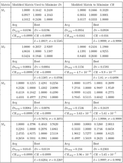
The proposed method is executed 10 times on each com-parison matrix. The result of the proposed method is initiated by getting the minimalDi andCR as presented in Table 3. It is obtained from performing the first two steps, which are described in Section 3.1. The best result of the 10 experiments is given for the values of Di, CR,

Table 3

Modified Matrix Used to MinimizeDi andCR

Matrix Modified Matrix Used to MinimizeDi Modified Matrix to MinimizeCR

M1 1.0000 0.1642 0.2438 1.0000 0.1666 0.3320

6.0917 1.0000 4.1043 6.0034 1.0000 3.0001

4.1012 0.2436 1.0000 3.0117 0.3333 1.0000

Avg Best Avg Best

Diavg= 0.0196 Di= 0.0196 Diavg= 0.0934 Di= 0.0938

CRavg= 0.0999 CR= 0.0999 CRavg= 0.0161 CR= 0.016

δ= 1.0917;σ= 0.5585 δ= 1.9999;σ= 0.9998

M2 1.0000 0.2057 2.9207 1.0000 0.2416 1.1900

4.8616 1.0000 5.1387 4.1391 1.0000 4.9255

0.3424 0.1946 1.0000 0.8403 0.2030 1.0000

Avg Best Avg Best

Diavg= 0.0004 Di= 0.0004 Diavg= 0.1156 Di= 0.1593

CRavg= 0.0999 CR= 0.0999 CRavg= 4.7×10−10 CR= 9.9×10−15

δ= 0.1387;σ= 0.0706 δ= 1.81;σ= 0.6898

M3 1.0000 0.1215 2.4281 0.2256 1.0000 0.1375 1.0001 0.2699

8.2326 1.0000 5.4302 2.0090 7.2716 1.0000 6.9887 1.9549

0.4118 0.1842 1.0000 0.4390 0.9999 0.1431 1.0000 0.2775

4.4331 0.4977 2.2781 1.0000 3.7045 0.5115 3.6042 1.0000

Avg Best Avg Best

Diavg= 0.0084 Di= 0.0076 Diavg= 0.1536 Di= 0.1619

CRavg= 0.0999 CR= 0.0999 CRavg= 3.63×10−5 CR= 5.61×10−5

δ= 0.7674;σ= 0.3073 δ= 1.9998;σ= 0.9999

M4 1.0000 4.3796 0.4043 3.7620 1.0000 3.0003 0.5260 2.0013

0.2283 1.0000 0.2076 1.6861 0.3333 1.0000 0.1746 0.6658

2.4735 4.8175 1.0000 2.5118 1.9012 5.7277 1.0000 3.8125

0.2658 0.5931 0.3981 1.0000 0.4997 1.5019 0.2623 1.0000

Avg Best Avg Best

Diavg= 0.0145 Di= 0.0118 Diavg= 0.216 Di= 0.2303

CRavg= 0.0999 CR= 0.0999 CRavg= 3.96×10−4 CR= 5.65×10−7

δ= 0.6204;σ= 0.2267 δ= 1.9997;σ= 0.9992

(Continued)

δ, and σ. The averages of the 10 experiments for the values ofDi andCR are also shown asDiavgandCRavg.

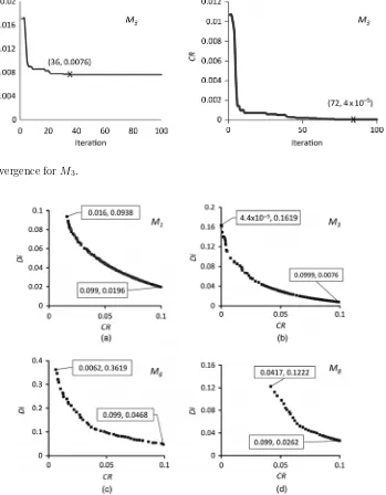
Figure 4 shows the convergence history of matrixM3.Both Di and CR quickly converge (within 100 iterations). Di and CR start to become optimal in iterations 36 and 72, respectively.

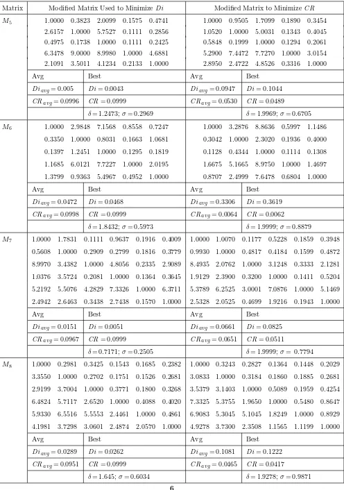
Some matrices, especially large ones, are diﬃcult to make perfectly consistent. M5,M7, andM8 have minimal CR values of 0.0489, 0.0511, and 0.0417, respectively. Besides the big size comparison matrix, those that limited

(6)

Table 3 (Continued)

Matrix Modified Matrix Used to MinimizeDi Modified Matrix to MinimizeCR

M5 1.0000 0.3823 2.0099 0.1575 0.4741 1.0000 0.9505 1.7099 0.1890 0.3454

2.6157 1.0000 5.7527 0.1111 0.2856 1.0520 1.0000 5.0031 0.1343 0.4045 0.4975 0.1738 1.0000 0.1111 0.2425 0.5848 0.1999 1.0000 0.1294 0.2061 6.3478 9.0000 8.9980 1.0000 4.6881 5.2900 7.4472 7.7270 1.0000 3.0154 2.1091 3.5011 4.1234 0.2133 1.0000 2.8950 2.4722 4.8526 0.3316 1.0000

Avg Best Avg Best

Diavg= 0.005 Di= 0.0043 Diavg= 0.0947 Di= 0.1044

CRavg= 0.0996 CR= 0.0999 CRavg= 0.0530 CR= 0.0489

δ= 1.2473;σ= 0.2969 δ= 1.9969;σ= 0.6705

M6 1.0000 2.9848 7.1568 0.8558 0.7247 1.0000 3.2876 8.8636 0.5997 1.1486

0.3350 1.0000 0.8031 0.1663 1.0681 0.3042 1.0000 2.3020 0.1936 0.4000

0.1397 1.2451 1.0000 0.1295 0.1819 0.1128 0.4344 1.0000 0.1114 0.1308

1.1685 6.0121 7.7227 1.0000 2.0195 1.6675 5.1665 8.9750 1.0000 1.4697

1.3799 0.9363 5.4967 0.4952 1.0000 0.8707 2.4999 7.6478 0.6804 1.0000

Avg Best Avg Best

Diavg= 0.0472 Di= 0.0468 Diavg= 0.3306 Di= 0.3619

CRavg= 0.0998 CR= 0.0999 CRavg= 0.0064 CR= 0.0062

δ= 1.8432;σ= 0.5973 δ= 1.9999;σ= 0.8879

M7 1.0000 1.7831 0.1111 0.9637 0.1916 0.4009 1.0000 1.0070 0.1177 0.5228 0.1859 0.3948

0.5608 1.0000 0.2909 0.2799 0.1816 0.3779 0.9930 1.0000 0.4817 0.4184 0.1599 0.4872

8.9970 3.4382 1.0000 4.8056 0.2335 2.9089 8.4935 2.0762 1.0000 3.1248 0.3333 2.1281

1.0376 3.5724 0.2081 1.0000 0.1364 0.3645 1.9129 2.3900 0.3200 1.0000 0.1411 0.5204

5.2192 5.5076 4.2829 7.3326 1.0000 6.3711 5.3789 6.2525 3.0001 7.0876 1.0000 5.1469

2.4942 2.6463 0.3438 2.7438 0.1570 1.0000 2.5328 2.0525 0.4699 1.9216 0.1943 1.0000

Avg Best Avg Best

Diavg= 0.0151 Di= 0.0051 Diavg= 0.0661 Di= 0.0825

CRavg= 0.0967 CR= 0.0999 CRavg= 0.0651 CR= 0.0511

δ= 0.7171;σ= 0.2505 δ= 1.9999;σ= 0.7794

M8 1.0000 0.2981 0.3425 0.1543 0.1685 0.2382 1.0000 0.3243 0.2827 0.1364 0.1448 0.2029

3.3550 1.0000 0.2702 0.1751 0.1526 0.2681 3.0833 1.0000 0.3184 0.1860 0.1885 0.2681

2.9199 3.7004 1.0000 0.3771 0.1800 0.3268 3.5379 3.1403 1.0000 0.5089 0.1959 0.4254

6.4824 5.7117 2.6520 1.0000 0.4088 0.4020 7.3325 5.3755 1.9650 1.0000 0.5480 0.8647

5.9330 6.5516 5.5553 2.4461 1.0000 0.4861 6.9083 5.3045 5.1045 1.8249 1.0000 0.8929

4.1981 3.7298 3.0601 2.4874 2.0570 1.0000 4.9278 3.7300 2.3508 1.1565 1.1199 1.0000

Avg Best Avg Best

Diavg= 0.0289 Di= 0.0262 Diavg= 0.1081 Di= 0.1222

CRavg= 0.0951 CR= 0.0999 CRavg= 0.0465 CR= 0.0417

(7)

Figure 4. Process of convergence forM3.

Figure 5. Pareto graphs for: (a)M1, (b)M3, (c)M6, and (d)M8.

matrix diﬃcult. Further, in chasing the minimal CR, sometimes the tendency of the value element matrix is changed. It can be shown on M6. The original a51 and

a52 values of M6 are 2 and 0.5, respectively. In other words, the DM had an original opinion that alternative 5 dominates alternative 1 with a value of 2 (a51= 2), and alternative 5 is dominated by alternative 2 with value 0.5 (a52= 0.5). However, to obtain a goodCR, the DM should change these values to 0.8707 and 2.4999 fora51 anda52, respectively. This shows that alternative 5 is dominated by alternative 1 with a value of 0.8707 (a51= 0.8707), and alternative 5 dominates alternative 2 with a value of 2.4999 (a52= 2.4999). After obtaining the minimalCR and Di, the third step of the proposed method is executed to get the non-dominated CR–Di nodes. By using PSO, for each value CR, the optimal Di can be obtained. This proposed method thus successfully generates some nodes as solutions.

(8)

Table 4

Comparison of PSO+Taguchi [14] and Proposed Method

Matrix Di CR δ σ

PSO+T Our PSO+T Our PSO+T Our PSO+T Our

Method Method Method Method

M1 0.064 0.0654 0.028 0.0279 2.1366 1.7369 1.0036 0.9531

M2 0.013 0.0127 0.0298 0.0376 0.6484 0.9015 0.2738 0.3993

M3 0.0821 0.0811 0.0107 0.0158 2.3501 1.9997 0.9546 0.9999

M4 0.0923 0.0921 0.0121 0.0144 1.7250 1.6833 0.7260 0.7399

M5 0.1106 0.1044 0.0079 0.0489 3.9616 1.9969 1.2905 0.2969

M6 0.1941 0.1938 0.0125 0.0219 3.6980 1.9999 1.1043 0.8798

M7 0.1119 0.0825 0.0042 0.0511 4.2326 1.9999 1.3741 0.8879

M8 0.1808 0.1222 0.0067 0.0417 4.0869 1.927 1.4659 0.9871

5. Conclusion

This work proposed a multi-objective approach that uses PSO to modify inconsistent comparison matrices. TheDi and theCR are minimized. The minimalDi is pursued to maintain the original opinion of the DM, while the small consistent ratio (CR) is pursued to chase the perfect logic of the opinion DM. PSO is found to be eﬀective at minimiz-ingDi andCR and obtained the optimal relationDi–CR (non-dominated solution) for repairing inconsistent matri-ces. Furthermore, PSO also exhibited fast processing to obtain convergence. The proposed method provides many alternative acceptable consistent matrices for repairing an inconsistent matrix. However, due to the many various combinations of Di and CR required to get a consistent matrix, we can give the weight for both Di and CR to represent the scale priority.

In the future, considering the PSO performance, a study that focuses on solving in more two objective func-tions to repair inconsistent comparison matrices would be interesting research.

Acknowledgement

This work was supported in part by the National Science Council, Taiwan, under Contract Nos. NSC 102-2219-E-006-001, MOST E-197-034, and MOST 103-2221-E-006-145-MY3

References

[1] T.L. Saaty, The analytic hierarchy process (New York, NY: McGraw-Hill, 1980).

[2] F. Chiclana, E. Herrera-Viedma, S. Alonso, and F. Herrera, Cardinal consistency of reciprocal preference relations: A char-acterization of multiplicative transitivity,IEEE Transactions on Fuzzy Systems,17, 2009, 14–23.

[3] S. Siraj, L. Mikhailov, and J. Keane, A heuristic method to rectify intransitive judgments in pairwise comparison matrices, European Journal of Operational Research,216, 2012, 420–428. [4] Y. Dong, G. Zhang, W.-C. Hong, and Y. Xu, Consensus models for AHP group decision making under row geometric mean

prioritization method, Decision Support Systems, 49, 2010, 281–289.

[5] S.M. Chen, T.E. Lin, and L.W. Lee, Group decision mak-ing usmak-ing incomplete fuzzy preference relations based on the additive consistency and the order consistency, Information Sciences,259, 2014, 1–15.

[6] Y. Xu, J.N. Gupta, and H. Wang, The ordinal consistency of an incomplete reciprocal preference relation, Fuzzy Sets and Systems, 246, 2014, 62–77.

[7] M. Xia, Z. Xu, and J. Chen, Algorithms for improving con-sistency or consensus of reciprocal [0, 1]-valued preference relations,Fuzzy Sets and Systems,216, 2013, 108–133. [8] Z. Xu and Q. Da, An approach to improving consistency

of fuzzy preference matrix, Fuzzy Optimization and Decision Making,2, 2003, 3–12.

[9] A. Ishizaka and M. Lusti, An expert module to improve the consistency of AHP matrices, International Transactions in Operational Research,11, 2004, 97–105.

[10] J.F. da Serra Costa, A genetic algorithm to obtain consistency in analytic hierarchy process,Brazilian Journal of Operations and Production Management,8, 2011, 55–64.

[11] D. Ergu, G. Kou, Y. Peng, and Y. Shi, A simple method to improve the consistency ratio of the pair-wise comparison matrix in ANP, European Journal of Operational Research, 213, 2011, 246–259.

[12] W. Ma, A practical approach to modify pair wise comparison matrices and two criteria of modificatory eﬀectiveness,Journal of Science and Systems Engineering,4, 1994, 37–58.

[13] C.C. Lin, W.C. Wang, and W.D. Yu, Improving AHP for construction with an adaptive AHP approach (A3

),Automation in Construction,17, 2008, 180–187.

[14] I. Yang, W.C. Wang, and T.I. Yang, Automatic repair of inconsistent pairwise weighting matrices in analytic hierarchy process,Automation in Construction, 22, 2012, 290–297. [15] X. Zeshui and W. Cuiping, A consistency improving method in

the analytic hierarchy process,European Journal of Operational Research,116, 1999, 443–449.

[16] D. Cao, L. Leung, and J. Law, Modifying inconsistent compari-son matrix in analytic hierarchy process: A heuristic approach, Decision Support Systems,44, 2008, 944–953.

[17] J. Ma, Z.P. Fan, Y.P. Jiang, J.Y. Mao, and L. Ma, A method for repairing the inconsistency of fuzzy preference relations, Fuzzy Sets and Systems,157, 2006, 20–33.

[18] J.F. Kennedy, J. Kennedy, and R.C. Eberhart,Swarm intelli-gence (Burlington, MA: Morgan Kaufmann, 2001).

(9)

[20] K.E. Parsopoulos, D.K. Tasoulis, and M.N. Vrahatis, Multi-objective optimization using parallel vector evaluated particle swarm optimization, Proc. IASTED Int. Conf. on Artificial Intelligence and Applications (AIA 2004), Innsburk, 2004, 823–828.

[21] C.A.C. Coello and M.S. Lechuga, MOPSO: A proposal for multiple objective particle swarm optimization,Proc. Congress on Evolutionary Computation, CEC’02, Honolulu, 2002, 1051– 1056.

[22] C.A.C. Coello, G.T. Pulido, and M.S. Lechuga, Handling multiple objectives with particle swarm optimization, IEEE Transactions on Evolutionary Computation,8, 2004, 256–279. [23] Z. Xiao Hua, M. Hong Yun, and J. Li Cheng, Intelligent particle swarm optimization in multiobjective optimization,The 2005 IEEE Congr. on Evolutionary Computation, 2005, 714–719. [24] T.L. Saaty and L.G. Vargas, Models, methods, concepts and

applications of the analytic hierarchy process, Kluwer Academic Publisher, Boston, 2001.

[25] T.L. Saaty, Decision making for leaders: the analytical hi-erarchy process for decisions in a complex world, Life Time Learning Publications, Belment, California, 1982.

Biographies

Abba Suganda Girsang is cur-rently a Ph.D. student from Indonesia in the Institute of Com-puter and Communication Engi-neering, Department of Electrical Engineering and National Cheng Kung University, Tainan, Taiwan, since 2009. He graduated bache-lor from the Department of Elec-trical Engineering, Gadjah Mada University (UGM), Yogyakarta, Indonesia, in 2000. He then con-tinued his masters degree in the Department of Computer Science in the same university in 2006–2008. He was a staﬀ consultant programmer in Bethesda Hospital, Yogyakarta, in 2001 and also worked as a web developer in 2002–2003. He then joined the faculty of Department of Informatics Engineering in Janabadra University as a lecturer in 2003. He also taught some subjects at some universities in 2006– 2008. His research interests include swarm intelligence, combinatorial optimization, and decision support system.

Chun-Wei Tsai received the Ph.D. degree in Computer Sci-ence and Engineering from Na-tional Sun Yat-sen University, Kaohsiung, Taiwan, in 2009. He was the adjunct lecturer with the Department of Information Management, National Pingtung Institute of Commerce and Com-munication Art, Tung Fang Insti-tute of Technology from 2004 to 2007, and 2005 to 2009, respec-tively. He was a postdoctoral fellow with the Department of Electrical Engineering, National Cheng Kung University, Tainan, Taiwan, before joining the faculty of the Applied Geoinformatics and the Information Technology, Chia Nan University of Pharmacy and Science, Tainan, Taiwan, in 2010 and 2012, respectively. He joined the faculty of

the Department of Computer Science and Information Engineering, National Ilan University, Yilan, Taiwan, as an assistant professor in 2014. His research interests in-clude computational intelligence, data mining, information retrieval, and Internet technology.