Reconfigurable Systems
Yi Lu, Thomas Marconi, Koen Bertels, and Georgi Gaydadjiev
Computer Engineering
Delft University of Technology, The Netherlands
{yilu,thomas,k.l.m.bertels,georgi}@ce.et.tudelft.nl
Abstract. Given the FPGA-based partially reconfigurable systems, hardware tasks can be configured into (or removed from) the FPGA fabric without interfer-ing with other tasks runninterfer-ing on the same device. In such systems, the efficiency of task scheduling algorithms directly impacts the overall system performance. By using previously proposed 2D scheduling model, existing algorithms could not provide an efficient way to find all suitable allocations. In addition, most of them ignored the single reconfiguration port constraint and inter-task dependen-cies. Further more, to our best knowledge there is no previous work investigating in the impact on the scheduling result by reusing already placed tasks. In this pa-per, we focus on online task scheduling and propose task scheduling solution that takes the ignored constraints into account. In addition, a novel “reuse and partial reuse” approach is proposed. The simulation results show that our proposed so-lution achieves shorter application completion time up to 43.9% and faster single task response time up to 63.8% compared to the previously proposedstuf f ing
algorithm.
1
Introduction
The reconfigurability of the FPGA has received much more attentions from various fields in the last decade. Usually, the FPGA is treated as a slave component in a recon-figurable system, when required, the complete FPGA is configured to offload the main processor. In this way, the FPGA can be easily managed as a solid part. With the devel-opment of the partially reconfigurable FPGAs, only the necessary part of the FPGA can be partially reconfigured when needed. By doing this, such partially reconfigurable sys-tems can provide real multi-task function. The partial reconfiguration technology brings higher FPGA resource usage and faster partial reconfiguration time, but also introduce a need of an efficient scheduler to manage the hardware tasks.
Offline and online solutions can be used to solve this problem. In an offline so-lution, the scheduling decision is optimized when the application is compiled. In an online solution, the information of each task (e.g. execution time, configuration time) is unknown until it arrives. The online solution provides more adaptivity to various ap-plications and avoids the application profile step, which is time-consuming. The online scheduler should, at runtime, assign a required time period to the arrival task. During
J. Becker et al. (Eds.): ARC 2009, LNCS 5453, pp. 216–230, 2009. c
this time period the task can be loaded and execute on the FPGA. The efficiency of the online scheduler will directly impact the overall performance of the whole system. In this paper, we focus on this online task scheduling and propose our solution.
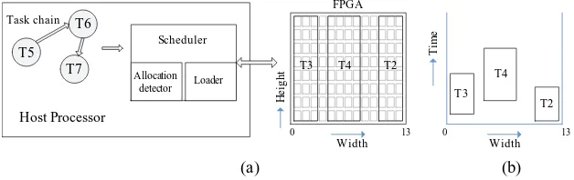
In our solution, the basic configuration unit of the target FPGA is a column with the complete height of the FPGA. This configuration is supported by the popular Xilinx Virtex FPGA. Each task used in our system occupies a set of continuous columns. In this way, the size of a task can be only represented by its width. Then the task scheduling can be processed by using the 2D scheduling model (referred as2D modelin this paper) described in [10]. As shown in Figure 1(b), in this model, the horizontal axis stands for the width of the FPGA and the vertical axis represents time. Each task can be treated as a rectangle in which the height represents the time (e.g. execution time and configuration time of the task) and the width keeps its original meaning. The scheduling problem now is similar to the strip packing as presented in [10]. Based on the 2D model, in this paper, we propose our solution to the online task scheduling problem. The main contributions of our solution are:
– to provide a modified algorithm which is suitable for searching the complete set of free allocations(stored as maximum free rectangles) on the 2D model;
– to present an example scheduling heuristic implied on the found allocations; – to demonstrate a “reuse and partial reuse” approach;
In section 2, related work and our observation are presented. Thereafter, we detail our proposal in section 3. In section 4, we present the simulation results and evaluate its performance while comparing against previously proposedstuf f ing algorithm [10]. Finally, we conclude this paper and discuss future works in section 5.
T5 T6
T7
Host Processor
Scheduler
Allocation detector
Task chain
Loader
FPGA
T3 T4 T2
Width
He
ig
h
t
0 13
T2 T4
T3
Ti
m
e
Width
(a) (b)
13 0
Fig. 1.The system architecture and scheduling model
2
Related Work
proposed and evaluated in their work. However, their algorithms can not find all suit-able scheduling positions for arrival tasks. In some cases, the arrival task is assigned to a later start time although there are other allocations allowing it to start earlier. Their algorithms also ignored the hardware constraint brought by the single reconfiguration port on the single-context FPGA (e.g. Xilinx FPGA), which will bring serious resource conflict when implementing the algorithms on real hardware. Zhou et al. [15] proposed a“window-based stuffing” online scheduling algorithm which is based on the 2D model from [10]. In this algorithm, for each arrival task, a time interval (the start time and the end time are decided according to the parameters of the arrival task) is defined on the 2D model. The occupied areas of scheduled tasks in the time window are passed to a placement algorithm (e.g. algorithms from [14][3][2]) to find available allocations for the arrival tasks. If found, the task is scheduled. This algorithm also ignored the hard-ware constraint as happened in [12]. Although the algorithm focused on a higher task acceptance ratio, it did not show obvious reduction of the completion time of the overall application, which reflects the overall performance of the partially reconfigurable sys-tems. In [4], Danne et al. proposed a scheduling algorithm for periodic real-time tasks. In this algorithm, the FPGA area is partitioned into one dimensional slots and each task has several variants with different size and execution time. All possible combinations of available tasks are measured by the utilization metrics which is defined in the algo-rithm. Then the combination of tasks with minimum resource usage will be loaded into the proper slot. In [7], Jeong et al. described an ILP algorithm. Although their ILP ap-proach considers prefetch and the hardware constraint of a single configuration port, the real hardware usage is not taken into account when implementing scheduling. In some cases, although the ILP shows successful task scheduling result, the assigned areas on the FPGA are not continuous, which actually leads a fail result.
By investigating the related works, we noticed that, firstly, when the online task scheduling problem is handled by using the 2D model, there is no suitable algorithms searching available allocations as we described above (e.g.[12] [10]). The previous proposed allocation searching algorithms (e.g.[14] [5]) can not serve well for the 2D model. (We will detail the reasons later in section 3). Secondly, in order to make the 2D model simple, most proposed scheduling algorithms ignored the reconfiguration port constraint. In this case, applications using such scheduling results will probably fail when running on the real hardware (detail explanation is in section 3). Thirdly, previously proposed online scheduling algorithms have not investigated the task reuse. However, the task reuse is the most direct way to decrease the reconfiguration overhead and is practical for many applications (details in section 3.5). Fourthly, task dependency is not well supported by the proposed algorithms, most algorithms used a large number of random independent tasks as their testbench.
3
Our Proposal
In this section we first present the unsuitability of the previously proposed algorithms aiming to find free allocations when they work on the 2D model. Then, the modified flow scanning (FS) algorithm [9] which is suitable for the 2D model is detailed. Next, the approach to overcome the configuration port constraint is detailed. Thereafter, a “best fit” scheduling heuristic is described. Last the “reuse and partial reuse” approach is presented.
In our solution, the base part is the algorithm which can find the complete set of free allocations. The “best fit” scheduling heuristic is an example of using the found free allocations, other heuristics can also be implied(e.g. we use the found free allocations in a different way when implementing the “reuse and partial reuse”, which is detailed in section 3.5). In our solution, the allocation searching algorithm and ”reuse and partial reuse” are highlighted.
3.1 Allocation Searching Algorithms
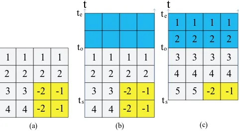
The previously proposed algorithms(e.g. [14] [5]) aiming to find the complete set of available free allocation are mostly based on the 2D matrix model. As shown in Fig-ure 2(a), the target is modeled as a 2D matrix, all cells are encoded with meaningful information(e.g. the negative value is assigned to the occupied area, and the positive value is to the free area). By processing the information of all cells, the complete set of free allocations can be found. These algorithms work well for the target models which have exact height and width (e.g. FPGA and multi-processor mesh). However, when im-plementing such algorithms on the 2D model, things become much more complicated. As shown in Figure 2(b), if a task arrives attsand is expected to complete byte, in
or-der to find all available allocations between this interval by using the algorithms based on the matrix model, information in almost all the cells has to be updated as shown in Figure 2(c). In addition, thetsandtewill probably be different for every task, which
means the size of the matrix has to be changed and all the information encoded in the cells has to be recalculated and updated every time a task arrives.
1
3.2 Modified Flow Scanning Algorithm
In [9], we previously proposed the flow scanning (FS) algorithm which finds the com-plete set of maximum free rectangles on the FPGA at runtime. To achieve this, the FS algorithm only need the positions of placed tasks and the width and height of the FPGA. In this work, the original FS algorithm was modified to be easily implied to the 2D model. The modified FS (mF S) algorithm is use to find all suitable allocations in the 2D model for arrival tasks. In this section, we will describe how themF Salgorithm works on the 2D model.
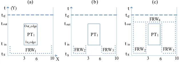
We start the description with an example to explain how themF Sworks on the 2D model as shown in the Figure 3. Assume that a new task arrives at timetsand is
ex-pected to complete by timete. An maximum free rectangle betweentsandteis needed
to allocate this task. In the beginning, an initialF RW1 is created at the task arrival timets(theF RW in themF Sis defined as a rectangle which has no top line and can
only be expanded upwards). The bottom of thisF RW1istsand it covers the complete width of the model, as shown in Figure 3(a). The scanning flow which is fromtstote
in thetdirection, will reach the in-edge1of a previously placed task 1 (P T
1) at timetin in thetdirection (shorthandAt time = tin:), the initialF RW1is overlapped with this edge inX direction, so it becomes a maximum free rectangle (0, 10,ts,tin) (in this
paper, we define such maximum free rectangle asscheduling rectangle (sRectangle)). Thereafter, two newF RWs are created for the non-overlapping area, as shown in Fig-ure 3(b), theF RW2andF RW3.At time = tout: the out-edge of taskP T1is met at this level, so the out-edge process is performed, which creates a newF RW:F RW4shown in Figure 3(c).At time = te: when reaching the top edge (te), which is defined as an
in-edge, all existingF RWs are transferred to maximum free rectangles with top att=
te. During the scanning process described above, totally four sRectangles were found:
(0, 10,ts,tin), (0, 3,ts,te), (6, 10,ts,te) and (0, 10,tout,te).
In themF S, there are two basic processes as shown in above example, the in-edge process and out-edge process. The in-edge process happens when the scanning flow
(b) (c)
reaches an in-edge and the out-edge process is called when leaving an out-edge. In the in-edge process, if aF RW is overlapped with an in-edge in theX direction, a sRectangle is created by adding to theF RW a top line at the height of the in-edge. NewF RW(s) will also be created if theF RW is not fully overlapped with the in-edge. In the out-edge process, only one newF RW is created with the bottom at the same height as the out-edge. Every time when a task arrives, a searching interval is set, which is the time period between thetsandte. By implying themF Sto the 2D model,
we do not need to rebuild the meaningful matrix every time. The available allocations are found only by runningmF Sto scan the searching interval.
3.3 Reconfiguration Port Scheduling
The reconfiguration port is a hardware interface located on the FGPA to implement the run-time partial reconfiguration. On current FPGAs (e.g. Xilinx FPGAs), only one reconfiguration port is supported, which means that the configuration of tasks is a se-quential process. As shown in Figure 4 (a), three tasksP T1,P T2andP T3arrive atts and are to be scheduled on the same FPGA. If the availability of the reconfiguration port on the FPGA is not taken into account, the three tasks are scheduled as shown in Figure 4 (b), which can be treated as a simple strip packing problem. However, if we check the availability of the reconfiguration port shown in Figure 4 (c), it is obvious that the configuration of theP T3can not start at timets, because the reconfiguration
port is occupied by the P T1. So the scheduling result shown in Figure 4 (b) is not feasible in reality. A reasonable scheduling result is shown in the Figure 4 (d). Fig-ure 4 (e) reflects the availability of the reconfiguration port after scheduling the three tasks.
In our algorithm, a reconfiguration port checking process is added to avoid the con-fliction of the reconfiguration port scheduling. After the mFS finds the complete set of sRectangles, the reconfiguration port checking process can be run to check the conflic-tion between the reconfiguraconflic-tion port availability and the sRectangles. If there is any conflict, the temporal values of the related sRectangles will be reset. As shown in Fig-ure 5 (b), the checking process finds that the start time (ts) of originalR2is overlapped with the configuration time ofP T1andP T2. Consequently, the start time ofR2is reset to the value shown in the figure.
1
PT
ts
(a)
3
PT t
1
PT
2
PT
ts
3
PT t
(b)
2
PT
1
T
2
T
3
T
t t
(c) (d) (e)
Configuration time
3.4 Best Fit Scheduling Heuristic
In our solution, the scheduling heuristics can be various. We are not aiming to provide a specific scheduling heuristic for all applications. Because by using our mFS algorithm, all available allocations on the 2D model can be easily found, we can implement various heuristics to use these found allocations for different applications.
In this paper, we will give an example scheduling heuristic, the best fit. The best fit heuristic is to schedule the arrival task into an available sRectangle which results in less fragmentation and better time performance in the 2D model. Based on our observa-tion, we created equation (1). For all available allocations, we calculate theirBFvalue by using equation (1), then the best fit one is chosen according to the values. In equa-tion (1),Atask stands for the arrival time of a task;Stask represents the starting time
for the task running on the FPGA;TwidthandRwidthare the width of the task and the
chosen sRectangle respectively; theEoverlapstands for the length of overlapped edges
between placed tasks and the new task when placed in a chosen rectangle and theEtask
is the perimeter of the arrival task.
BF =Atask
Stask ×
Twidth Rwidth ×
Eoverlap Etask
...(1)
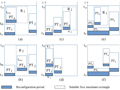
Equation (1) consists of three components which reflects the time issue and the de-fragmentation requirements by using the 2D model, as shown in the Figure 5.P Tx(x
= 1,2...) stands for the placed task;P Tais the arrival task;Rx(x = 1,2...)is the suitable
sRectangle to locate the arrival task. In Figure 5 (a) (b), when a new taskP Taarrives
atts and is expected to complete by te, R1 andR2 are both suitable for the P Ta.
However, allocatingP Tain these suitable sRectangles will give different response time
and completion time. In our approach, we allocate theP TaintoR2in order to achieve shorter response time as well as the earlier completion time. Corresponding to the equa-tion (1), for various suitable allocaequa-tions, we choose the one with biggest AtaskStask value. In Figure 5 (c) (d), it can be observed that when the arrival task is placed in the suitable sRectangle with shorter width (R1), less fragmentation will be created. This reflects the requirement of largerRwidthTwidth value. In Figure 5 (e) (f), we observed that when placed the arrival task with more overlapped edges with placed tasks, less fragmentation will be created. Corresponding to the equation (1), the chosen sRectangle should have largest value ofEoverlapEtask .
In equation (1), the three situations are taken into account by multiplying them to-gether. For the best fit heuristic, we calculate theBF values of all suitable sRectangles for the arrival task and choose the one with largest value. We want to mention again that the best fit heuristic is an example to show how to use these found sRectangles, it can achieve good performance as shown later in section 4, however, for different situations, we believe that different heuristics can be applied to the found sRectangles in order to achieve better results.
3.5 Reuse and Partial Reuse
ts
Reconfiguration period Suitable free maximum rectangle
t t t
Fig. 5.Heuristics for defragmentation
hide this overhead(e.g. [1] [6]). Most previous work focus on hiding the reconfigura-tion time to the users, however, the reconfigurareconfigura-tion port is still occupied by these tasks. In most current FPGAs, only one reconfiguration port is supported, which means that the reconfiguration is a sequential process. This reflects that the overall configuration time of all hardware modules in an application is a fixed value. When the number of the hardware modules is increased and the size of modules becomes bigger (usually because the logic of modules become complicated), this overall configuration time will become much longer (sometime even comparable to the execution time of applications). This is one of the critical reasons to limit the use of partially reconfigurable systems in real applications. So, the most efficient way to avoid the reconfiguration overhead is to support reuse of the tasks which have been already placed on the FPGA as much as possible. During our investigation to many applications, we noticed that different hardware function modules in the same application usually work on the same objects, which makes the logic of each module can be reused by others (e.g. the pixel operation functions in H.264 applications). In addition, many hardware modules contain common functions (e.g. multiply, memory address generator). Given these reasons, the reuse of placed tasks is efficient and practical. In this paper, we propose our task reuse and par-tial reuse (RP R) approach. The “reuse” means to use the logic of placed taskTp to
implement the arrival taskTa, which save the configuration time of the arrival task. The
partial reuse happens in two situations: 1) the logic of placed taskTpcan not implement
the complete function of the arrival taskTabut a part; 2)Tp can implement the
func-tion ofTa, butTpwill be removed before it can complete the execution forTa. When
the partial reuse is applied, the logic ofTpis used forTa, meanwhile, theTa itself is
also configured on the FPGA. Once theTa is ready, the partially processed data will
be transferred fromTp toTa, thenTa can complete the computation. In this way, the
partial reuse hide the configuration time ofTato the user.
1
Fig. 6.Heuristics for reuse
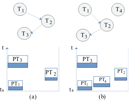
should exist on the FPGA as long as possible. Given this, we apply another heuristic to allocate the arrival tasks as shown in the Figure 6. For the data independent task or the first task in a task graph, it is placed at the bottom left corner of the sRectangle with fastest response time, e.g. theP T4andP T1shown in Figure 6 (b). For the tasks having data dependence, each task is placed as far as possible (in the horizontal direction) from its ancestor task, e.g.P T1,P T2andP T3shown in Figure 6 (a).
An example of theRP Rprocess is shown in the Figure 7. Assume that the taskP T1 toP T4have already been scheduled and the taskP T1 meets the requirements of be-ing reused by the taskP Taarriving atts. In the 2D model, if the height of sRectangle
above theP T1is no less than the value of execution time when reusingP T1forP Ta, theP T1 can be directly reused for execution ofP Ta afterP T1completes, as shown in Figure 7 (a). On the contrary, if the height is less than the value, the partial reuse approach can be implied. The difference of implementing scheduling solution with and without partial reuse approach is shown in Figure 7 (b) and (c). In Figure 7 (b),P Tais
placed as usual, Instead, the Figure 7 (c) shows that the result of implementing partial reuse approach. Comparing the task ending timete, the partial reuse approach gives
1
Partial reconfiguration period Extra period for the task setting
Fig. 7.Reuse and partial reuse
was presented in [8]. By using this type of busmacro system, tasks placed on the FPGA have the same bus interface and share the buses. The connecting interface of tasks to the buses is same as the interface of custom unit in the “Molen” architecture [11].
The overall algorithm is shown as follow:
Algorithm:
Input: arrival task, searching starting time, searching ending time
ifReuse function checking is truethen
assign the arrival task to the reusable module;
else ifPartial reuse checking is truethen
assign a part of calculation of the arrival task to the reusable module; searching all free allocations for the rest of the arrival task;
implying scheduling heuristic to choose an allocation;
else
searching all free allocations;
checking conflict of the reconfiguration port; implying scheduling heuristic;
end if
4
Experimental Evaluation
The target FPGA is Xilinx Virtex II XC2V4000 FPGA which contains 80(row) x 72(col-umn) CLBs. The total configuration time of the complete FPGA is 39.15ms (SelectMAP port at 50MHz). On the FPGA, there are total 2156 frames, which is the minimum con-figuration unit. All the CLBs in one column use 22 frames. The reconcon-figuration time of one column is calculated by using the equation shown in [1]:Tcolumn=(frames per
col-umn) x ((total configuration time) / (total frames)) = 22 x (39.15 / 2156) = 0.40ms. The partial reconfiguration time of each task will be calculated based on these data.
The tasks we used in the experiment were created via two steps. In the first step, VHDL codes of real hardware tasks (e.g.f multandupdate2
for G721 encoder, DCT and AES) were generated by DWARV3[13]. Then they were synthesized by Xilinx ISE
and implemented on the “Molen” [11]. In this step, we collected information of the real
2Thef multperforms table look-up and theupdateis control dominated processing of multiple
scalar variables.
3
hardware tasks (e.g. task size, execution time). Considering that the limit number of real tasks, we generated large amount of theoretic tasks in the second steps. Firstly, we set the ranges of task size and execution time based on the information collected from the real tasks. Then the size and execution time of theoretic tasks were randomly chosen in these ranges. The task size is in the range[5..20]columns and the execution time is in the range[1.00..50.00]ms. The configuration time of a task is related to its size, e.g. for a task occupied 5 columns, the configuration time of the task is 0.40 x 5 = 2.00 ms. Our proposed scheduling approach supports both data dependent and independent tasks. We used task graph to represent tasks as shown in the Figure 7. The number of tasks in each task graph was randomly chosen in the range[1..5].
Usually, the partially reconfigurable systems can be categorized into two types. The hardware operation only and the hardware-software (Hw/Sw) cooperation. In the first type, all tasks in an application can only run on the hardware target (e.g. FPGAs). For the second type which supportsHw/Swcooperation, each task in the application can either run on the hardware target or the general purpose processor (GPP). In the experiment, we considered both types. In the simulation ofHw/Swcooperation type, two extra parameters of tasks were given: the software execution time of a task (Tset)
and the dummy time (Tdummy) of a task. The Tset is the task execution time when
it runs on the GPP and theTdummy represents the time that a task can wait for the
scheduling on the FPGA. If the scheduling can not be made within theTdummy, the
task will run on the GPP. For the tasks generated via DWARV, the two parameters are collected from the real hardware implementation. For the randomly created tasks, the
Tsetis randomly set as 3 to 5 times of the execution time of the task, and theTdummy
is randomly set as 0.5 to 2.5 times of the execution of the task.
In the experiment, the performance of our proposed approaches (BFandRP R) and
thestuf f ing[10] were evaluated. The originalstuf f ingalgorithm did not support
data dependent tasks and reconfiguration port check, in order to fairly compare our approaches to thestuf f ingalgorithm, we modified thestuf f ingalgorithm to support these features. All algorithms were programmed using C, and executed under Linux 2.6 with Intel(R) Pentium(R) 4 CPU 3.00GHz. All algorithms were evaluated in term of application completion time and single task response time.
4.1 Application Completion Time
The application completion time (ACT) is defined as the completion time of the ap-plication. In each simulation run, firstly an application was generated by randomly cre-ating the task graph and tasks (each application consists of 50 task graphs). Then the
Stuf f ing,BF andRP Rwere implied to the application respectively and theACT
were measured. Totally, 1000 simulation runs were implemented and the results shown in the table 1 were evaluated by using the following equation:
A
B =
AETB−AETA
AETB ×
100% ...(2)
The AB stands for the comparison of A to B and its value is calculated by the right side of equation (2). The positive value means that theAETAis shorter thanAETB, which
reflects that algorithm ‘A’ outperforms algorithm ‘B’ (similarly, ‘B’ is better than ‘A’ for a negative value). If comparing serval algorithms to ‘B’, the best algorithm will show the closest value to “100%”.
As shown in the table 1, the “Average” column gives the average value of the 1000 simulation runs, and the “Best” and “W orst” columns show the largest and smallest values respectively. It can be observed in the third row that averagely theBF outper-forms thestuf f ingby 11. 3% in term ofACT, and the worst and best cases among the 1000 simulation runs are 3. 9% and 20.4% respectively. TheBF outperforming
stuf f ing can be explained with 2 reasons: 1) the mFS algorithm used in BF can
find all suitable sRectangles for arrival tasks, which can not be granted bystuf f ing; 2) by using equation (1), less fragmentation, shorter response time and shorter com-pletion time can be achieved for the allocation of each task. When implementing our
RP Rtechnology, averagely around 20% tasks are reused or partially reused in an ap-plication. As shown in the second and fourth rows of the table 1, theRP Rachieved better performance compared toBF andstuf f ing. This is because when reusing a placed taskTpfor an arrival taskTa, the reconfiguration time ofTais removed. In
ad-dition, the reconfiguration port can be used to load other tasks during the period when theTashould be loaded (theTashould be loaded whenRP Ris not implied). Further
more, although extra communication time is required when implying partial reuse, it helps to achieves shorter completion time and response time as described earlier in the section 3.5.
Table 1.Comparison of ACT
Average Best Worst RPR / BF 28. 9% 39.1% 11. 6% BF / stuffing 11. 3% 20.4% 3. 9% RPR / stuffing 34.7% 43. 9% 20.8%
4.2 Single Task Response Time
The single task response time (STRT) is defined as the time interval represented by:
Tresponse-Tarrival. TheTarrivalstands for the arrival time of a task, and theTresponse
is the starting time of the task configuration or the starting time of the execution when reusing a placed task. The STRT is an very important character to measure the system performance especially for the real-time systems. The results shown in the table 2 are in the same format as the table 1. The results are calculated by using equation (3) which holds the similar explanation as the equation (2).
A
B =
ST RTB−ST RTA
ST RTB ×
100% ...(3)
Table 2.Comparison of STRT
Average Best Worst RPR / BF 41.6% 61.6% 12. 5% BF / stuffing 11.7% 23.4% 2.4% RPR / stuffing 49. 9% 63.8% 28. 5%
reductions of STRT are averagely around 28. 9% and 34.7% compared to theBF and
stuf f ing respectively. The explanation for the BF and RP Rhaving better STRT
results can also be referred to the reasons described for the comparison of ACT results. In our simulation, the execution time for scheduling a task is in a range from 0.09ms to 0.13ms, averagely 0.11ms. Compared to the reconfiguration time of tasks used in our simulation (which is from 2.0ms to 8.0ms), the time used for a single task scheduling is acceptable.
4.3 Hw / Sw System Scenario
In the previous two subsections, we assumed that all tasks can only run on the hard-ware and we presented the comparison ofACT andST RT among theBF,RP Rand
stuf f ing. In this subsection, the system is assumed to run in the Hw/ Sw mode. In
our approach, when a task arrives, the mFS algorithm finds all suitable sRectangles for the task in the required searching interval, which is defined as:Tarrive+Tdummy
+Tconf iguration +Texecution. TheTarrive stands for the arrival time of the task, the Tconf igurationis the configuration time of the task and theTexecution is the hardware
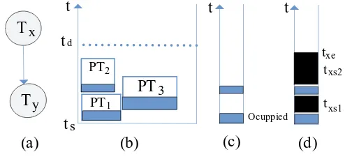
execution time of the task. By using the mFS algorithm, all suitable sRectangles in the required time interval are aware, the schedule of a task to the FPGA or the GPP can be processed immediately when the task arrives. In previously proposed algorithms, because of unknowing all suitable sRectangles, if an arrival task can not be scheduled to the FPGA immediately, it has to wait until the end of the dummy time. During that period, if any suitable allocation found, it will be scheduled to the FPGA, otherwise, it will be assigned to the GPP after the dummy time.
In the simulation, we used a linked list to represent the availability of the GPP. Each node in the linked list shows a continuous free period of the processor. If an arrival task is assigned to the GPP, the task is scheduled in the nearest node(s). An example of scheduling a task to the GPP is shown in the Figure 8. When taskTxandTyarrive
atts, the mFS can not find a suitable allocation for theTxduring the time interval [Ts Td], so the Tx is decided to run on the GPP. The resource availability of the FPGA
and the GPP are shown in Figure 8 (b)(c) respectively. According to Figure 8 (c), the
Tx is scheduled on the GPP into two time interval txs1 and txs2. The Ty which is
data-dependent with theTxcan only run after thetxe(the completion time of theTx).
(a)
1
PT
2
PT
t
s3
PT
t
(b)
x
T
y
T
t
t
(c)
(d)
t
dtxs2
txs1 txe
Ocuppied
Fig. 8.Task software execution
Table 3.comparison of ACT for Hw/Sw mode
Average Best Worst RPR/BF 20.74% 39.9% 0.3% BF/stuffing -4.5% 15.5% -28.5% RPR/stuffing 21.2% 54.2% -6.7%
HW/ SW mode, although in the beginning, theBF scheduled more tasks to the FPGA compared tostuf f ing, the free time periods of the reconfiguration port become much smaller fragmentation, which results in unusable for the later tasks. On the contrary, although thestuf f ingcreated more fragmentation on the 2D model, it kept the relative longer free time periods of reconfiguration port, which helped to achieve a good overall performance. Then we simulated theRP R, as expected, by decreasing the impaction from availability of reconfiguration port, theP RPachieved averagely 21.2% reduction ofACTcompared to thestuf f ing.
5
Conclusion and Future Work
In this paper, we proposed an online task scheduling solution for the FPGA-based par-tially reconfigurable systems. Building upon our allocation search approach, various scheduling heuristics could be applied to different situations. In addition out “reuse and partial reuse” approach showed the potential to shorter the ACT and STRT. Our experi-mental validation has shown that our solution has up to 43.9% shorter ACT and 63.8% faster STRT compared to thestuf f ing algorithm. In the future, our work will focus on: (i) implementing the “reuse and partial reuse” method on our “Molen” prototype board; (ii) considering the heterogenous resource distribution on the FPGA.
References
1. Banerjee, S., Bozorgzadeh, E., Dutt, N.: Physically-aware hw-sw partitioning for reconfig-urable architectures with partial dynamic reconfiguration. In: The Proceeding of the 42nd Design Automaion Conference (DAC), June 13-17, pp. 335–340 (2005)
2. Bazargan, K., Kastner, R., Sarrafzadeh, M.: Fast template placement for reconfigurable com-puting systems. IEEE Design and Test of Computers 17, 68–83 (2000)
3. Chiu, G., Chen, S.: An efficient submesh allocation scheme for two-dimensional meshes with little overhead. IEEE Trans. Parallel and Distributed Systems 10, 471–486 (1999)
4. Danne, K., Platzner, M.: Partitioned scheduling of periodic real-time tasks onto reconfig-urable hardware. In: The proceedings of the 20th International Parallel and Distributed Pro-cessing Symposium (IPDPS), April 25-29 (2006)
5. Handa, M., Vemuri, R.: An efficient algorithm for finding empty space for online fpga place-men. In: Proceedings of the 41st annual conference on desing automation, San Diego, pp. 960–965 (June 2004)
6. Hauck, S.: Configuration prefetch for single context reconfigurable coprocessors. In: Pro-ceedings of the sixth International Symposium on Field Programmable Gate Arrays (FPGA 1998), pp. 65–74 (1998)
7. Jeong, B., Yoo, S., Lee, S., Choi, K.: Hardware-software cosynthesis for run-time incremen-tally reconfigurable fpgas. In: The Proceeding of the Asia and South Pacific Design Automa-tion Conference (ASP-DAC), pp. 169–174 (2000)
8. Kalte, H., Porrmann, M.: Context saving and restoring for multitasking in reconfigurable systems. In: Proceedings of the International Conference on Field Programmable Logic and Applications (FPL), pp. 223–228 (2005)
9. Lu, Y., Marconi, T., Gaydadjiev, G., Bertels, K.: An efficient algorithm for free resource management on the fpga. In: Proceedings of Design, Automation and Test in Europe (DATE 2008), Munich, Germany (March 2008)
10. Steiger, C., Walder, H., Platzner, M.: Operating systems for reconfigurable embedded plat-forms: Onlline scheduling of real-time tasks. IEEE Transactions on Computers 53 (Novem-ber 2004)
11. Vassiliadis, S., Wong, S., Gaydadjiev, G., Bertels, K., Kuzmanov, G., Panainte, E.M.: The molen polymorphic processor. IEEE Transactions on Computers archive 53 (November 2004)
12. Walder, H., Platzner, M.: Reconfigurable hardware operating systems: From concepts to re-alizations. In: Proc. Int’l Conf. Eng. of Reconfigurable Systems and Algorithms (ERSA), pp. 284–287 (2003)
13. Yankova, Y., Kuzmanov, G., Bertels, K., Gaydadjiev, G., Lu, Y., Vassiliadis, S.: Dwarv: Delft workbech automated reconfigurable vhdl generator. In: International Conference on Field Programmable Logic and Applications (FPL), August 27-29, pp. 697–701 (2007)
14. Yoo, S., Youn, H., Shirazi, B.: An efficient task allocation scheme for 2d mesh architectures. IEEE Trans. Parallel and Distributed Systems 8, 934–942 (1997)