Principal Whitened Gradient for Information
Geometry
Zhirong Yang and Jorma Laaksonen
Laboratory of Computer and Information Science, Helsinki University of Technology, P.O. Box 5400, FI-02015 TKK, Espoo, Finland
Abstract
We propose two strategies to improve the optimization in information geometry. First, a local Euclidean embedding is identified by whitening the tangent space, which leads to an additive parameter update sequence that approximates the geodesic flow to the optimal density model. Second, removal of the minor components of gra-dients enhances the estimation of the Fisher information matrix and reduces the computational cost. We also prove that dimensionality reduction is necessary for learning multidimensional linear transformations. The optimization based on the principal whitened gradients demonstrates faster and more robust convergence in simulations on unsupervised learning with synthetic data and on discriminant anal-ysis of breast cancer data.
Key words: information geometry, natural gradient, whitening, principal components, Riemannian manifold
1 Introduction
Denote J an objective function to be minimized and θ its parameters. The steepest descent update rule
θnew=θ−η∇J(θ) (1)
with η a positive learning rate is widely used for minimization tasks because it is easy to implement. However, this update rule performs poorly in machine learning problems where the parameter space is not Euclidean. It was pointed
Email addresses: [email protected](Zhirong Yang),
out by Amari that the geometry of the Riemannian space must be taken into account when calculating the learning directions (Amari, 1998). He suggested the use of natural gradient (NAT) updates in place of the ordinary gradient-based ones:
θnew=θ−ηG(θ)−1∇J(θ), (2) where G(θ) is the Riemannian metric matrix. Optimization that employs natural gradients generally requires much less iterations than the conventional steepest gradient descent (ascend) method.
Information geometry is another important concept proposed by Amari and Nagaoka (2000), where the Riemannian metric tensor is defined as the Fisher information matrix. The application of the natural gradient to information geometry leads to substantial performance gains in Blind Source Separation (Amari, 1998), multilayer perceptrons (Amari, 1998; Amari et al., 2000), and other engineering problems that deal with statistical information. Neverthe-less, many of these applications are restricted by the additive Gaussian noise assumption. Little attention has been paid on incorporating the specific prop-erties of information geometry to facilitate general optimization.
We propose here to improve the natural gradient by a novel additive update rule called Principal Whitened Gradient (PWG):
θnew =θ−ηGˆ(θ)−12∇J(θ). (3)
The square root and hat symbols indicate two strategies we use, both of which are based on a crucial observation that the Fisher information is the covari-ance of gradient vectors. First, we identify a local Euclidean embedding in the parameter space by whitening the tangent space at the current estimate of θ. The additive update sequence with whitened gradients results in a better approximation to the geodesic flow. The choice of learning rates also becomes easier in the Euclidean embedding. Second, the whitening procedure is ac-companied with removal of minor components for computational efficiency and for better estimation of the Fisher information with finite data. We also prove that dimensionality reduction is necessary for learning a great variety of multidimensional linear transformations.
We demonstrate the advantage of PWG over NAT by three simulations, two for unsupervised learning and one for supervised. The first task in our exper-iments is to learn the variance of a multivariate Gaussian distribution. The second is to recover the component means of a Gaussian mixture model by the maximum likelihood method. The last one is to learn a matrix that maximizes discrimination of labeled breast cancer data. In all simulations, the updates with principal whitened gradients outperform the original natural gradient results in terms of efficiency and robustness.
2007) by the same authors. In this paper we include the following new contri-butions:
• We propose to interpret the Fisher information metric as the local change of the Kullback-Leibler divergence. A formal derivation based on Taylor series is also provided.
• We point out that the Fisher information matrix is the covariance of or-dinary online gradients and this property is invariant of linear transforma-tions. This result provides a new justification for the employed prewhitening procedure.
• We clarify the motivation for discarding the minor components as the prin-cipal ones correspond to the directions where the local information change is maximized.
• We use three different simulations. A new kind of simulation is added to demonstrate the learning of variance. The learning on Gaussian mixtures is extended to a two-dimensional case. We also use another data set for the discriminative learning experiment.
The remaining of the paper is organized as follows. We first provide a brief of the natural gradient and information geometry, as well as the concept of geodesic updates in Section 2. In Section 3, we present two strategies to im-prove the optimization in information geometry. Next we demonstrate the performance of the proposed method with simulations on learning a Gaussian mixture model and discriminating breast cancer data in Section 4. Finally the conclusions are drawn in Section 5.
2 Background
2.1 Natural Gradient and Information Geometry
A Riemannian metric is a generalization of the Euclidean one. In an m-dimensional Riemannian manifold, the inner product of two tangent vectors
u and v, at point θ, is defined as
hu,viθ≡
m
X
i=1
m
X
j=1
[Gij] (θ)uivj =uTG(θ)v, (4)
where G(θ) is a positive definite matrix. A Riemannian metric reduces to Euclidean when G(θ) =I, the identity matrix.
approach in the Euclidean space by seeking a vector a that minimizes the linear approximation of the updated objective (Amari, 1998)
J(θ) +∇J(θ)Ta. (5)
Natural gradient employs the constraint ha,aiθ = ǫ instead of the Euclidean norm, where ǫ is an infinitesimal constant. By introducing a Lagrange multi-plier λ and setting the gradient with respect toa to zero, one obtains
a= 1
2λG(θ) −1
∇J(θ). (6)
Observing a is proportional to G(θ)−1∇J(θ), Amari (1998) defined the
nat-ural gradient
∇NATJ(θ)≡G(θ)−1∇J(θ) (7)
and suggested the update rule
θnew =θ−ηG(θ)−1∇J(θ) (8)
with η a positive learning rate.
Many statistical inference problems can be reduced to probability density esti-mation.Information geometry proposed by Amari and Nagaoka (2000) studies a manifold of parametric probability densities p(x;θ), where the Riemannian metric is defined as the Fisher information matrix
[Gij] (θ) =E
(
∂ℓ(x;θ) ∂θi
∂ℓ(x;θ) ∂θj
)
. (9)
Here ℓ(x;θ) ≡ −logp(x;θ). Amari also applied the natural gradient update rule for the optimization in the information geometry by usingJ(θ) =ℓ(x;θ) as the online objective function, which is equivalent to the maximum likelihood approach (Amari, 1998). Similarly, the batch objective function can be defined to be the empirical mean ofℓ(x;θ) over x.
It is worth to note that the natural gradient method has been applied to other Riemannian manifolds. For example, Amari (1998) proposed to use the natural graident on the manifold of invertible matrices for the blind source separation problem. However, this is beyond the scope of information geometry. In this paper we only focus on the improvement in the manifolds defined by the Fisher information metric.
2.2 Geodesic Updates
curve θ≡θ(t) is a geodesic if and only if (Peterson, 1998)
are Riemannian connection coefficients. The geodesic with a starting point θ(0) and a tangent vector vis denoted by θ(t;θ(0),v). Theexponential map
of the starting point is then defined as
expv(θ(0))≡θ(1;θ(0),v). (12)
It can be shown that the length along the geodesic betweenθ(0) and expv(θ(0))
is |v|(Peterson, 1998).
The above concepts are appealing because a geodesic connects two points in the Riemannian manifold with the minimum length. Iterative application of exponential maps therefore forms an approximation of flows along the geodesic and the optimization can converge quickly.
Generally obtaining the exponential map (12) is not a trivial task. In most cases, the partial derivatives of the Riemannian tensor in (11) lead to rather complicated expression of Γk
ij and solving the differential equations (10)
there-fore becomes computationally infeasible. A simplified form of exponential maps without explicit matrix inversion can be obtained only in some special cases, for instance, when training multilayer perceptrons based on additive Gaussian noise assumptions (Amari, 1998; Amari et al., 2000). When the Rie-mannian metric is accompanied with left- and right-translation invariance, the exponential maps coincide with the ones used in Lie Group theory and can be accomplished by matrix exponentials (see e.g. Nishimori and Akaho, 2005). This property however does not hold for information geometry.
3 Principal whitened gradient
3.1 Whitening the Gradient Space
the covariance of these gradients. That is, the squared norm of a tangent vector
u is given by
kuk2G≡uTGu=uTE{∇∇T}u, (13)
The following theorem justifies that such a squared norm is proportional to the local information change alongu.
Theorem 1 Let u be a tangent vector at θ. Denote p ≡ p(x;θ) and pt ≡
p(x;θ+tu). For information geometry,
kukG ≡
√
uTGu=√2 lim
t→0
q
DKL(p;pt)
t , (14)
where DKL is the Kullback-Leibler divergence. The proof can be found in Appendix A.
Now let us consider a linear transformation matrix F in the tangent space. From the derivation in Appendix A, it can be seen that the first term in the Taylor expansion always vanishes, and the second remains zero under linear transformations. When connecting to the norm, the terms of third or higher order can always be neglected ift is small enough. Thus the local information change in the transformed space is only measured by the second-order term.
Another crucial observation is that the Hessian H of the Kullback-Leibler divergence can be expressed in the form of gradient vectors instead of the second order derivative. Thus we have the following corollary:
Corollary 1 Given a linear transformationu˜ =Fu, the Hessian in the trans-formed space
˜
H= ˜G≡E{∇˜∇˜T}=FE{∇∇T}FT, (15)
and
√
2 lim
t→0
q
DKL(p,p˜t)
t =
q
˜
uE{∇˜∇˜T}u˜ =ku˜k
˜
G, (16)
where p˜t ≡p(x;θ+tu˜).
This allows us to look for a proper Ffor facilitating the optimization.
Since the Fisher information matrixGis positive semi-definite, one can always decompose such a matrix as G = EDET by a singular value decomposition, where D is a diagonal matrix and ETE = I. Denote the whitening matrix
G−12 for the gradient as
G−12 =ED− 1
where
h D−12
i
ii=
1/√Dii if Dii>0
0 if Dii= 0
. (18)
With F=G−12, the transformed Fisher information matrix becomes
E{∇˜∇˜T}=G−1
2E{∇∇T}G−12 =I. (19)
That is, the whitening matrix locally transforms the Riemannian tangent space into its Euclidean embedding:
ku˜k2G˜ = ˜uTE{∇˜∇˜T}u˜ = ˜uTu˜ =ku˜k2. (20)
The optimization problem in such an embedding then becomes seeking a tan-gent vector a that minimizes
J(θ) +h∇J˜ (θ)iTa (21)
under the constraint kak2 = ǫ. Again by using the Lagrangian method, one can obtain the solution
a=− 1
2λ∇J˜ (θ), (22) which leads to an ordinary steepest descent update rule in the whitened tan-gent space:
θnew =θ−η∇J˜ (θ). (23)
By substituting ˜∇=G−12∇, we get the whitened gradient update rule:
θnew =θ−ηG(θ)−1
2∇J(θ). (24)
The update rule (24) has a form similar to the natural gradient one (2) except the square root operation on the eigenvalues of the Fisher information matrix at each iteration. We address that such a difference brings two distinguished advantages.
Second, we can see that the learning rate η in (2), or the corresponding La-grange multiplierλin (6), is a variable that depends not only onθandJ, but also on G(θ). This complicates the choice of a proper learning rate. By con-trast, selecting the learning rate for the whitened gradient updates is as easy as for the ordinary steepest descent approach becauseη in (24) is independent of the local Riemannian metric.
3.2 Principal Components of Whitened Gradient
The singular value decomposition used in (17) is tightly connected toPrincipal Component Analysis (PCA) which is usually accompanied with dimensionality reduction for the following two reasons.
First, the Fisher information matrix is commonly estimated by the scatter matrix with n <∞ samples x(i):
G≈ 1
n
n
X
i=1
∇θℓ(x(i);θ)∇θℓ(x(i);θ)T. (25)
However, the estimation accuracy could be poor because of sparse data in high-dimensional learning problems. Principal Component Analysis is a widely-applied method for reducing such kind of artifacts by reconstructing a positive semi-definite matrix from its low-dimensional linear embedding. In our case, the principal directionw maximizes the variance of the projected gradient:
w= arg max kuk=1E{(u
T∇)2}. (26)
According to Theorem 1,wcoincides with the direction that maximizes local information change:
E{(uT∇)2}=uTE{∇∇T}u= 2
lim
t→0
q
DKL(p;pt) t
2
, (27)
wherep≡p{x(i)};θ,pt≡p{x(i)};θ+tu, andθ is the current estimate. By this motivation, we preserve only the principal components and discard the minor ones that are probably irrelevant for the true learning direction. More-over, the singular value decomposition (17) runs much faster than inverting the whole matrixGwhen the number of principal components is far less than the dimensionality ofθ (Golub and van Loan, 1989).
Second, dimensionality reduction is sometimes motivated by structural rea-sons. Consider a problem where one tries to minimize an objective of the form
where W is an m ×r matrix. Many objectives where Gaussian basis func-tions are used and evaluated in the linear transformed space can be reduced to this form. Examples can be found in Neighborhood Component Analysis (Goldberger et al., 2005) and in a variant of Independent Component Analysis (Hyv¨arinen and Hoyer, 2000). The following theorem justifies the necessity of dimensionality reduction for this kind of problems.
Denoteξi =kWTx(i)k2in (28) andfi = 2∂J(ξi)/∂ξi. The gradient ofJ(x(i);W)
with respect toW is denoted by
∇(i)≡ ∇WJ(x(i);W) =fix(i)
x(i)T W. (29)
Them×r matrix∇(i) can be represented as a row vector
ψ(i)T by concate-nating the columns such that
ψk(i+() l−1)m =∇(kli), k= 1, . . . , m, l= 1, . . . , r. (30)
Piling up the rows ψ(i)T, i= 1, . . . , n, yields ann×mr matrix Ψ.
Theorem 2 Suppose m > r. For any positive integer n, the column rank of
Ψ is at most mr−r(r−1)/2.
The proof can be found in Appendix B. In words, no matter how many samples are available, the matrix Ψ is not full rank when r > 1, and neither is the approximated Fisher information matrix
G≈ 1
nΨ
TΨ. (31)
That is,Gis always singular for learning multidimensional linear transforma-tions in (28). G−1 hence does not exist and one must employ dimensionality reduction before inverting the matrix.
Suppose ˆD is a diagonal matrix with the q largest eigenvalues of G, and the corresponding eigenvectors form the columns of matrix ˆE. The geodesic update rule with Principal Whitened Gradient (PWG) then becomes
θnew =θ−ηGˆ−12ψ(i), (32)
where ˆG = ˆEDˆEˆT. For learning problems (28), the newW is then obtained
4 Simulations
4.1 Learning of Variances
First we applied the NAT update rule (2) and our PWG method (3) to the estimation of a 30-dimensional zero-mean Gaussian distribution
p(x;w) =
where the parameter wd is the inverted variance of the dth dimension.
Al-though there exist methods to obtain the estimate in a closed form, this sim-ulation can serve as an illustrative example for comparing NAT and PWG.
We drew n = 1,000 samples from the above distribution. The negative log-likelihood of the ith sample is
ℓ(x(i);w)≡ −
of which the partial derivative with respect to wk is
∂ℓ(x(i);w)
With these online gradients, we approximated the Fisher information matrix by (25) and calculated the batch gradient
∇ ≡ 1
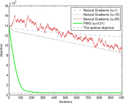
We first set the learning rateη = 1 in natural gradient updates. The whitening objective values in the iterative optimization are shown as the dot-dashed curve in Figure 1. The learning proceeds slowly and after 1,000 iterations the objective is still very far from the optimal one. Increasing the learning to η = 10 can slightly speed up the optimization, but a too large learning rate, e.g.η = 50, leads to a jagged objective evolution. Although the objective keeps decreasing in a long run, the resulting variance estimates are no better than the one obtained with η= 10.
0 100 200 300 400 500 600 700 800 900 1000
Natural Gradients (η=1) Natural Gradients (η=10) Natural Gradients (η=50) PWG (η=0.01) The optimal objective
Fig. 1. Learning the variances of a multivariate Gaussian distribution.
4.2 Gaussian Mixtures
Next we tested the PWG method (3) and the NAT update rule (2) on synthetic data that were generated by a Gaussian Mixture Model (GMM) of ten two-dimensional normal distributions N(µ(∗k),I), k = 1, . . . ,10. Here µ(∗k) were randomly chosen within (0,1)×(0,1). We drew 100 two-dimensional points from each Gaussian and obtained 1,000 samples in total. The true {µ(∗k)} values were unknown to the compared learning methods, and the learning task was to recover these means with the estimates{µ(k)}randomly initialized. We used the maximum likelihood objective, or equivalently the minimum negative log-likelihood
where C = 1000 log (2π)10/2 is a constant. We then computed the partial derivatives with respect to each mean:
Similarly, the batch gradient was the empirical mean of the online ones over i, and the Fisher information matrix was approximated by (25).
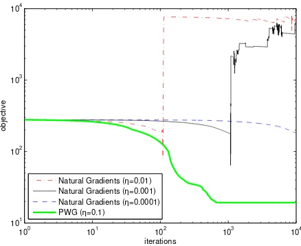
The dot-dashed line in Figure 2 shows the evolution of the objective when using natural gradient (2) with the learning rate η = 0.001. Although the negative likelihood is decreasing most of the time, the optimization is severely hindered by some unexpected upward jumps. We found 17 rises in the curve, among which the most significant four take place in the 1st, 546th, 856th and 971st rounds. Consequently the objective cannot converge to a satisfactory result.
One may think that the η = 0.001 could be too large for natural gradient updates and turn to a smaller one, e.g.η= 10−4. The training result is shown as the thin solid curve in Figure 2, from which we can see that the objective decreases gradually but slowly. Although the unexpected rises are avoided, the optimization speed is sacrificed due to the excessively small learning rate.
The objectives by using principal whitened gradient are also shown in Figure 2 (thick solid curve). Here we setη= 0.01 and seven principal components of the whitened gradient are used in (3). It can be seen thatJGMMdecreases steadily and efficiently. Within 18 iterations, the loss becomes less than 3,200, which is much better than the loss levels obtained by the natural gradient updates. The final objective achieved by PWG updates is 3,151.40—a value very close to the global optimum 3,154.44 computed by using the true Gaussian means
{µ(∗k)}.
4.3 Wisconsin Diagnostic Breast Cancer Data
We then applied the compared methods on the real Wisconsin Diagnostic Breast Cancer (WDBC) dataset which is available in UCI Repository of ma-chine learning databases (Newman et al., 1998). The dataset consists of n = 569 instances, each of which has 30 real numeric attributes. 357 samples are labeled asbenign and the other 212 as malignant.
Denote {(x(i), ci)}, x(i) ∈ R30, ci ∈ {benign,malignant} for the labeled data
pairs. We define here the Unconstrained Informative Discriminant Analysis
(UIDA) which seeks a linear transformation matrixWof size 30×2 such that the negative discrimination
JUIDA(W)≡ −
n
X
i=1
logp(ci|y(i)) (39)
predic-0 100 200 300 400 500 600 700 800 900 1000
Natural Gradients (η=0.001) Natural Gradients (η=0.0001) Principal Whitened Gradients
Natural Gradients (η=0.001) Natural Gradients (η=0.0001) Principal Whitened Gradients The optimal objective
Fig. 2. Learning a GMM model by natural gradient and principal whitened gradient in 1000 rounds (top) and in the first 100 rounds (bottom).
tive density p(ci|y(i)) is estimated by the Parzen window method:
width, and the transformation matrixW is constrained to be orthonormal. In this illustrative example we aim at demonstrating the advantage of PWG over NAT updates in convergence. We hence remove the orthonormality constraint for simplicity. By this relaxation, the selection of the Parzen window width is absorbed into the learning of the transformation matrix.
PWG is suitable for the UIDA learning since UIDA’s objective has the form (28). Letk denote a class index. First we compute the individual gradients
∇(i) = vectorize
By applying Taylor expansion in analog to the derivation in Appendix A, we can obtain
Then the learning direction is ˜∇ left-multiplied by the principal whitened components of G−P
kp(k)Gk.
100 101 102 103 104 101
102 103 104
iterations
objective
Natural Gradients (η=0.01) Natural Gradients (η=0.001) Natural Gradients (η=0.0001) PWG (η=0.1)
Fig. 3. Objective curves of discriminating WDBC data by using NAT and PWG.
speed becomes extremely slow and the UIDA objective is no less than 180 after 10,000 iterations.
By contrast, the proposed PWG method (3) demonstrates both efficiency and robustness in this learning task. From Figure 3, it can be seen that the negative discrimination keeps decreasing by using PWG with η = 0.1. We obtained
JUIDA < 200 after 40 iterations, and the best objective achieved by using PWG is 19.24 after 10,000 iterations.
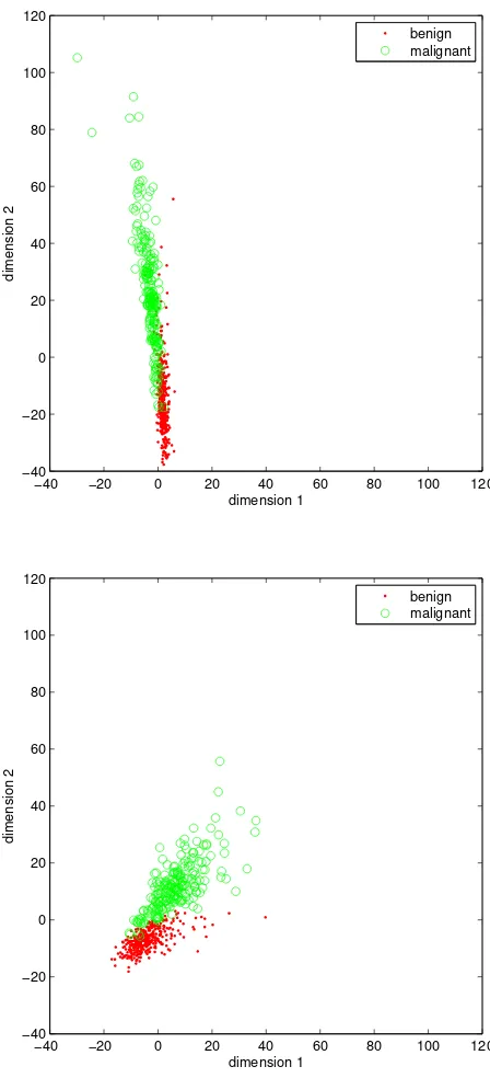
The projected data are displayed in Figure 4, where we used η = 0.001 for NAT and η = 0.1 for PWG. The results are examined after 500 iterations of both methods. We can see that the benign and malignant samples mainly distribute along a narrow line and are heavily mixed after the NAT updates, whereas the two classes are quite well separated by using the PWG method. The corresponding objective value is 229.04 by using NAT and 24.89 by PWG.
5 Conclusions
−40 −20 0 20 40 60 80 100 120 −40
−20 0 20 40 60 80 100 120
dimension 1
dimension 2
benign malignant
−40 −20 0 20 40 60 80 100 120
−40 −20 0 20 40 60 80 100 120
dimension 1
dimension 2
benign malignant
Fig. 4. WDBC data in the projected space. Top: 500 NAT updates withη= 0.001. Bottom: 500 PWG updates with η= 0.1.
both unsupervised and supervised learning.
(Yang, 1995). Another potential extension of the PWG update rule is to make it to accommodate additional constraints such as orthonormality or sparseness. Moreover, many conventional optimization techniques, such as the conjugate gradient, can be applied in the Euclidean embedding to further improve the convergence speed.
6 Acknowledgment
This work is supported by the Academy of Finland in the projects Neural methods in information retrieval based on automatic content analysis and rel-evance feedback and Finnish Centre of Excellence in Adaptive Informatics Research.
A Proof of Theorem 1
The proof follows the second order Taylor expansion of the Kullback-Leibler divergence aroundθ:
DKL(p;pt)≡
Z
p(x;θ) log p(x;θ) p(x;θ+tu)dx =DKL(p;p) + (tu)Tg(θ)
+1 2(tu)
TH(θ)(tu) +o(t2), (A.1)
where
g(θ) = ∂DKL(p;p
t)
∂θt
θt=θ
(A.2)
and
H(θ) = ∂ 2D
KL(p;pt) (∂θt)2
θt=θ
, (A.3)
with θt =θ+tu.
The first term equals zero by the definition of the divergence. Suppose the density function fulfills the mild regularity conditions:
Z ∂k
The second term also vanishes because
B Proof of Theorem 2
We apply the induction method on r. When r = 1, the number of columns of Ψis m. Therefore the column rank of Ψ, rankcol(Ψ), is obvious no greater than m×r−r×(r−1)/2 = m.
Now consider each of the matrices
˜
B(jk)≡B(j) B(k), j = 1, . . . , k−1. (B.2)
Notice that the coefficients
ρ≡w(1k), . . . , w(mk),−w(1j), . . . ,−w(mj) (B.3)
fulfill
ρTB˜(jk)= 0, j = 1, . . . , k−1. (B.4) Treating the columns as symbolic objects, one can solve the k −1 equations (B.4) by for example Gaussian elimination and then write out the last k−1 columns ofΨ(k) as linear combinations of the firstmr−(k−1) columns. That is, at most m−(k−1) linearly independent dimensions can be added when
w(k) is appended. The resulting column rank of Ψ(k) is therefore no greater than
Amari, S., 1998. Natural gradient works efficiently in learning. Neural Com-putation 10 (2), 251–276.
Amari, S., Nagaoka, H., 2000. Methods of information geometry. Oxford Uni-versity Press.
Amari, S., Park, H., Fukumizu, K., 2000. Adaptive method of realizing natural gradient learning for multilayer perceptrons. Neural Computation 12 (6), 1399–1409.
Goldberger, J., Roweis, S., Hinton, G., Salakhutdinov, R., 2005. Neighbour-hood components analysis. Advances in Neural Information Processing 17, 513–520.
Golub, G. H., van Loan, C. F., 1989. Matrix Computations, 2nd Edition. The Johns Hopkins University Press.
Newman, D., Hettich, S., Blake, C., Merz, C., 1998. UCI repository of machine learning databases
http://www.ics.uci.edu/∼mlearn/MLRepository.html.
Nishimori, Y., Akaho, S., 2005. Learning algorithms utilizing quasi-geodesic flows on the Stiefel manifold. Neurocomputing 67, 106–135.
Peltonen, J., Kaski, S., 2005. Discriminative components of data. IEEE Trans-actions on Neural Networks 16 (1), 68–83.
Peterson, P., 1998. Riemannian geometry. Springer, New York.
Yang, B., 1995. Projection approximation subspace tracking. IEEE Transac-tions on Signal Processing 43 (1), 95–107.