OPTIMIZATION OF FROZEN FOOD DISTRIBUTION USING GENETIC
ALGORITHMS
Widdia Lesmawati 1, Asyrofa Rahmi 2, Wayan Firdaus Mahmudy 3
Faculty of Computer Science, Universitas Brawijaya, Indonesia
E-mail: 1sos.widdia@gmail.com, 2asyrofarahmi@gmail.com, 3wayanfm@ub.ac.id
ABSTRACT
Nowadays, 30% of Indonesian consume frozen foods because it is more practical and efficient. The increase of demand requires a good distribution system. The distribution problem can be solved using genetic algorithms. Crossover method used in this study is one-cut point crossover, the mutation method used is reciprocal exchange mutation and the selection method used is elitism selection. The data used in this study is 15 of customers, 11 of product types, 5 vehicles and distance data between regions. From the tests, we found that optimal results are achieved using the population size of 1950, 700 generations, a combination of crossover rate (cr) = 0.5 and mutation rate (mr) = 0.6. The final result is a combination of the customer and vehicle order that distribute all products to all customers with the minimum total distance and cost.
Keywords: genetic algorithm, optimization, frozen food, distribution
1. INTRODUCTION
The distribution is an activity of transferring goods or products from the manufacturer to the customers. On the technical execution of the process, the distributor uses some vehicle as a carrier of the products. To minimize distribution cost, a good strategy is required. This strategy includes determining routes of the vehicles. The problem is called the Vehicle Routing Problem (VRP). The VRP is considered as a combinatorial optimization problem has been solved using various methods (Kumar & Panneerselvam 2012; Mahmudy 2014a).
On the technical execution of the distribution of goods, the distributor will use some of the vehicles as a carrier of goods to be distributed to customers. The different areas of customers require distributors to determine the route of travel distribution of goods. The main
objective of solving the problem is minimizing the distribution cost. A minimum distribution cost may be achieved by minimizing distribution routes and also minimizing used vehicles in the distribution process. In addition to these, the capacity of the vehicles should also be considered (Pitaloka, Mahmudy & Sutrisno 2014). The better the quality of the distribution process, the greater the benefits will be obtained.
Finding a solution in the distribution process is a part of decision-making process in supply chain management (Moon, Lee & Seong 2012). The various problem of distribution process has been addressed in the literature. For example, Hsu, Hung and Li (2007) address a distribution of perishable foods. The objective of this study is delivering the foods as soon as possible as their value will decrease during distribution. The objective can be achieved by minimizing the distribution routes of vehicles. A similar study is carried out by Osvald and Stirn (2008) that address the distribution of fresh vegetables.
This problem can be solved by many methods, one of them is Genetic Algorithm. The genetic algorithm is a search technique in computer science to provide optimal solutions to the complex issues such as planning and production scheduling, scheduling lectures, multi-traveling salesman problem (M-TSP) and the visit of efficient travel (Dipesh Mittal et al. 2015; Mahmudy, Marian & Luong 2013a; Widodo & Mahmudy 2010).
52 P-ISSN:2356-3109 E-ISSN: 2356-3117 on the increase in corporate profits in the form
of an increase in customers.
2. PROBLEM DESCRIPTION
Frozen food is a form of food through pickling process to be frozen so that it can last longer. This is done to slow down the decomposition by changing the water content remaining to ice that inhibited bacterial growth and food last longer (Brecker & Fricke 1999; Wang & Zou 2014).
Freezing food is not only done by farmers, fishermen or hunters. This freezing process creates a new business that attracted many people, especially housewives. In addition to the raw foods, freezing is also done for the half-cooked food.
In addition to providing convenience, the success of the frozen food business was also supported by a number of consumer’s interest. In addition to convenience, consumers prefer frozen food than fresh food because of better nutritional content.
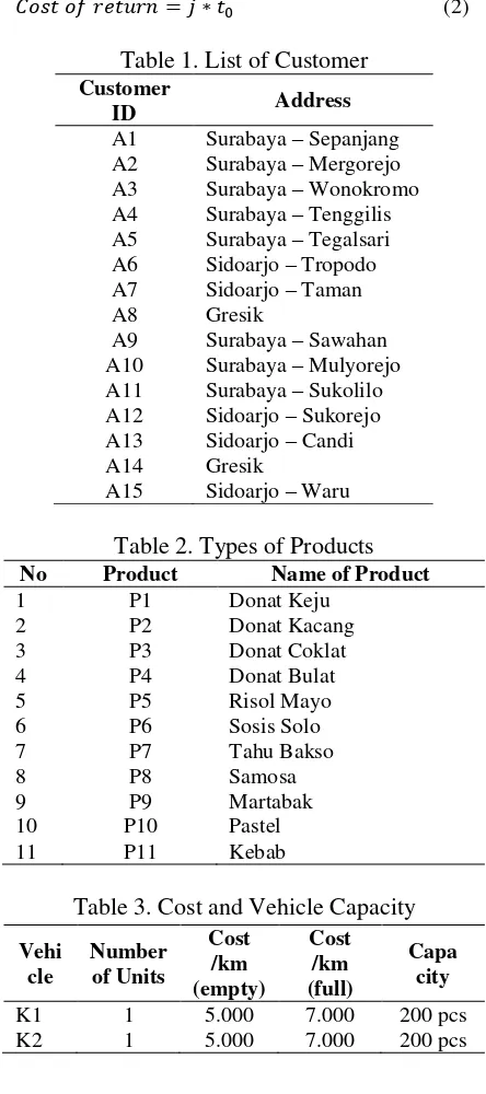
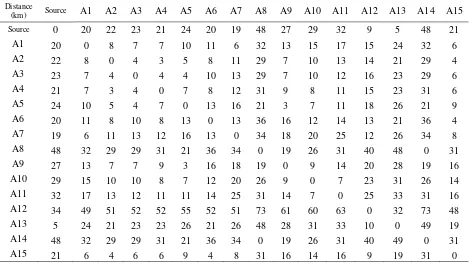
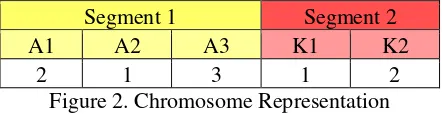
The data used in this study has several attributes, namely customer data, product data and distance data from household industry M-frozen snack. The third attribute is used to solve the problems of the distribution of the frozen food by knowing the distance between the customer and charge capacity based on the number of bookings. So the best solution based on the shortest distance, distribution costs and residual charge on the delivery of frozen foods show minimal results. The attributes used in the optimization process that customer data is shown in Table 1, the type of products are shown in Table 2, the transportation costs of the vehicle when full and empty and capacities described in Table 3, then Table 4 indicating the distance between the customer and the customer resources with one another.
Optimization distribution observed in this study only covers the area of Surabaya, East Java. While frozen food to be distributed is assumed to have the quality and the same survival time.
Distribution costs will be optimized in this research is the cost used by the distributor when the distribution of goods to customers. The distribution cost is calculated starting from the supplier to the customer (cost of going) at contents of the vehicle maximal (wmax). Costs
go can be calculated using the formula in equation (1) and equation (2) to calculate the departure and return journey cost respectively.
) )
(1) (2)
Table 1. List of Customer
Customer
Table 2. Types of Products
No Product Name of Product
Table 3. Cost and Vehicle Capacity
Table 4. Distance amongs Customers
Distance
(km) Source A1 A2 A3 A4 A5 A6 A7 A8 A9 A10 A11 A12 A13 A14 A15
Source 0 20 22 23 21 24 20 19 48 27 29 32 9 5 48 21
A1 20 0 8 7 7 10 11 6 32 13 15 17 15 24 32 6
A2 22 8 0 4 3 5 8 11 29 7 10 13 14 21 29 4
A3 23 7 4 0 4 4 10 13 29 7 10 12 16 23 29 6
A4 21 7 3 4 0 7 8 12 31 9 8 11 15 23 31 6
A5 24 10 5 4 7 0 13 16 21 3 7 11 18 26 21 9
A6 20 11 8 10 8 13 0 13 36 16 12 14 13 21 36 4
A7 19 6 11 13 12 16 13 0 34 18 20 25 12 26 34 8 A8 48 32 29 29 31 21 36 34 0 19 26 31 40 48 0 31
A9 27 13 7 7 9 3 16 18 19 0 9 14 20 28 19 16
A10 29 15 10 10 8 7 12 20 26 9 0 7 23 31 26 14
A11 32 17 13 12 11 11 14 25 31 14 7 0 25 33 31 16 A12 34 49 51 52 52 55 52 51 73 61 60 63 0 32 73 48 A13 5 24 21 23 23 26 21 26 48 28 31 33 10 0 49 19 A14 48 32 29 29 31 21 36 34 0 19 26 31 40 49 0 31
A15 21 6 4 6 6 9 4 8 31 16 14 16 9 19 31 0
3. OPTIMIZATION USING GAs
Frozen food distribution problem is solved using Genetic Algorithms. As one of the combinatorial algorithm, Genetic Algorithm is able to solve various problems by providing a solution that is near optimal (Mahmudy 2014b). There is a fleet of vehicles (K), a producer as a source, a number of customers (n), three kinds of products (A1, A2 dan A3) and a diverse customer demand (mi). Customers are
served in dots geographically dispersed so that it can be calculated the distance of each point as the distance between the customers (dij). Each
distance (i,j) has a certain costs (ci,j) assumed to
be symmetric, ie cij = cjiand on condition that cii
= 0. Shipping products to customers uses two vehicles with a payload capacity of uniform. Table 5 is a customer demand for each product from the manufacturer.
Table 5. Customer Demand
Customer Product 1
(P1)
Product 2 (P2)
Product 3 (P3)
A1 30 30 10
A2 30 10 40
A3 10 30 50
Besides the data request, the manufacturer also has the vehicles used to carry out the distribution process. Table 6 is the data of each vehicle.
Table 6. Data Cost Vehicle
Vehi cle
Number of Units
Cost /km (empty)
Cost /km (full)
Charge
K1 1 3.000 5.500 150 pcs K2 1 3.000 5.500 150 pcs
Figure 1 is a graph of the location of the three customers who book (A1, A2, and A3) and the distance between end-users.
54 P-ISSN:2356-3109 E-ISSN: 2356-3117
3.1 Chromosome Representation and Fitness Value
To explain chromosome representation, a simple case is given as an example. The process involves 3 customers (A1, A2, and A3) who book at 3 types of items (P1, P2, and P3). The distribution uses 2 vehicles which can carry 200 items at one time.
Representation of chromosomes uses permutations of the two segments. The first segment is a permutation-based customer with a certain length indicating the number of customers. While the second segment is a permutation-based vehicle with a certain length indicating the number of vehicles used to carry out the distribution process. This problem can be illustrated in Figure 2.
Segment 1 Segment 2
A1 A2 A3 K1 K2
2 1 3 1 2
Figure 2. Chromosome Representation
In Figure 2, the yellow color indicates the segment 1. The red color indicates the two gene segments 1 and 2. Segment 1 contains three genes, namely 2, 1 and 3 are a number of genes which means the distributor will serve A2 beforehand. Then the service is done to the A1 and the latter on the A3. Segment 2 consists of two genes that are represented in the last 2 digits on the chromosome, ie 1 and 2. This indicates that the service will be conducted by K1 A2 beforehand. If the charge on the K1 has been met then K2 will be filled. This process continues until all customers need are fulfilled.
Once the chromosomes are formed, the delivery of frozen foods (Sen et al. 2011). It is intended that the cost of distribution to each cost when empty or loaded. The fitness value is calculated based on the sum of the penalty and the total cost. The greater the value of the sum of the penalty and the total cost, then the fitness value obtained will be smaller. This is because
Table 7. Calculation of fitness
Vehicle Customer Capacity Residual
Charge Cost 2]. K1 is doing the distribution to the customer 1 (A1) with a maximum payload of 150 pcs. But K1 penalized because the charge on delivery is not optimal. Freight shipments in Q1 amounted to only 80 pcs so are the remaining 70 pcs in K1. This is called a penalty.
is 10 x (3000 + ((5500-3000) x 80/150)) = 10 x 4333.33 = 43333. Then the cost of distribution by K1 on the A1 is 15 x (3000 + ((5500 - 3000) x 70/150)) = 15 x 3666.67 = 55000. On this issue, the cost of which is used to return to the manufacturer accumulated by the customer last visited, namely A1. So the total cost of distribution to P1 K1 is 55000 + (20 x 3000) = 55000 + 60000 = 115000. The process of calculating the distribution of K-2 also has the same stage.
After the total penalties and cost of the problem are obtained, then the fitness value can be calculated using the equation previous fitness. The resulting fitness value is
3.2 Population Initialization
The system will generate initial population randomly which contain a number of individuals. The number is determined by predetermined variable named population size (popsize):
3.3 Crossover
One method to produce new individuals is is a cross exchange or crossover. Reproduction by using the crossover will produce a number of children (offspring) in accordance with cr (crossover rate) and its popsize. cr ratio is a proportion of children to be produced using crossover operator. The calculation of the amount obtained by multiplying cr and popsize. The method used is the one-cut point crossover. The initial process begins with the calculation of the child (offspring) that will be generated. Value cr on these problems is 0.6 with popsize of 5, the offspring resulting from crossover is a 0.6 x 5 = 3 offspring. Next, we chose two individuals at random to be the parents in the process of reproduction. Suppose individuals selected are individuals 3 and 5 shown in Table 8.
Table 8. Chosen Individual for Crossover
Parent Segment 1 Segment 2
P3 3 1 2 1 2
P5 3 2 1 2 1
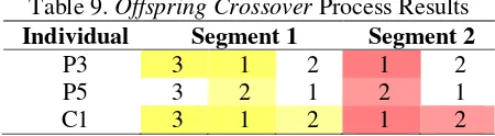
After the parent is selected, the next step is determinin the cut-off point at random in each segment. Table 9 is the process of cutting each of the parental chromosomes.
Table 9. OffspringCrossover Process Results Individual Segment 1 Segment 2
P3 3 1 2 1 2
P5 3 2 1 2 1
C1 3 1 2 1 2
Process crossover segment 1, are on the cutting-point-2 genes into the parent 1. Thus, two genes in the parent 1 to 2 first gene offspring on segment 1. The next step is checking the parent 2. If the gene in question is already present in offspring, then checking is proceed to the next gen. So we get the genetic make-up of offspring is 3 1, 2, 3 and 1 is derived from one parent while the 2 genes derived from parent 2.
Calculation of segment 2 has the same stages with the stages of the calculation of segment 1. The following is a list of crossover offspring result.
3.4 Mutation
Another way to produce offspring is by mutation. The number of children (offspring) generated in the process of mutation is determined by mr (mutation rate) and population size. Mr is a likelihood ratio to produce a child in a mutation. The calculation of the amount of child obtained by multiplying the mr and popsize. On this issue, the method used is the reciprocal exchange.
Reproduction of the problems in the previous section can be started with the calculation of the number of children (offspring) that will be generated. mr value is set to 0.4 with popsize 5, the offspring resulting from a mutation is a number of 0.4 x 5 = 2 offspring. Then we randomly choose one chromosome to be a parent in the process of reproduction. Example of selected individual in shown in Table 10.
Table 10. Chosen Individual for Mutation Individual Segment 1 Segment 2
56 P-ISSN:2356-3109 E-ISSN: 2356-3117 After the parent is selected, then determine
the two genes randomly in each segment. Table 11 is the selection of the parent chromosome genes in the process of mutation.
Table 11. Offspring Mutation Process Result Individual Segment 1 Segment 2
P2 2 1 3 2 1
C4 3 1 2 1 2
Mutations in done in one segment, the genes to be exchanged are the first gene and a third gene, ie 2 and 3. Therefore, when the composition of the parent gene segment 1 is 2 1 3 3 1 2 turn out to be the offspring. While the process of mutations in two segments, genes will be exchanged are the first and second gene, ie 1 and 2. Therefore, when the composition of the parent gene segment 2 is 2 1, is changed to 1 second in the offspring.
The second mutation process is carried out in the same manner as in the first mutation but using newly acquired individuals randomly from the population.
3.5 Selection
The selection process is doneto establish a new population by using selection methods elitism. Elitism selection method will select individuals of the initial population (the parent) and children (offspring) to get a new population on the population as much as the previous generation. This new population is the population with the best fitness value which will be the population in the next generation.
The selection process using the method of selection is elitism sort a collection of individuals and offspring based on the value of fitness. Once sorted the selected individuals with the best fitness number popsize
.
4. EXPERIMENTAL RESULT
Testing conducted to evaluate whether the genetic algorithm is able to solve the problems of optimization of the distribution of frozen foods. Based on the genetic algorithm parameter best results of the tests are expected to offer solutions that maximize and near optimal. Testing parameters of the genetic algorithm will be performed 10 times. Due to the nature of the stochastic algorithms that yield different solutions each run, the best results of
each test will be better if obtained from the average (Mahmudy, Marian & Luong 2013b).
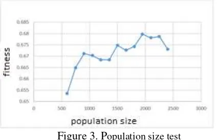
4.1 Testing of Population Size
The first stage in the numerical experiment is determining the best population size. In this stage, number of generation, cr,and mr are set to 100, 0.6 and 0.4 respectively. The testing result is presented in Figure 3.
Figure 3. Population size test
From the graph in Figure 3, it appears that the change in the value of the size of the population heavily influence the fitness value. The larger the size of the population, then the fitness value generated even greater. In testing with population size in 1950 resulted in the average highest fitness value, which is 0.67974382. Furthermore, the average fitness value obtained is not much different from the value average maximum. This is because the results of reproduction have the same resemblance to its parent.
4.2 Testing of Generation/Iteration
Figure 4. Chart of the test results from Generation / Iteration
From Figure 4, it appears that the change in the value of the generation heavily influence the fitness value is obtained. The greater the value of the generation / iteration, the computing time required increases. In the test with the value of the generation / iteration 100 generates the average highest fitness value, which is 0.68050289. Furthermore, the average fitness values obtained in the next generation is not much different from the value average maximum.
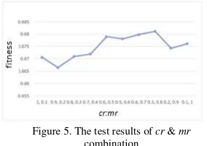
4.3 Testing of cr & mr Combination
cr and mr testing were conducted to determine the best combination of value to get the best fitness value. The best population size and the number of generations from previous test results will be used in testing combination of cr and mr as the parameters. cr is tested in the range of 1 to 0.1 contrasts to mr in the range between 0.1 to 1. Figure 5 shows the result of combination testing.
Figure 5. The test results of cr & mr combination
From the graph in Figure 5, the change in value cr and mr greatly affect the value of fitness. cr and mr combination determines the performance of the genetic algorithm in exploring and exploit the search space
(Mahmudy, Marian & Luong 2013b). cr and mr value will be different on each problem. In this study, combination of cr and mr to get value average highest fitness is cr = 0.3 and mr = 0.8 with the average highest fitness value is 0.681114481.
4.4 Testing using the Best Parameter
The last experiment is conducted to determine the best parameter best fitness value using the best parameter values from previous testing. The population size is 1950, the number of next-generation is 100 and the combination is cr = 0.3 with a value mr = 0.8. Figure 6 is the result of the test with the best parameters.
Figure 6. The test results with the best parameters
From the graph in Figure 6, it appears that the change in the value of fitness is not so significant. Fitness values obtained in testing using the best parameters fall in the range between 0.66 - 0.6927.
5. CONCLUSION
Genetic algorithms can be applied to a wide range of issues, including the distribution of frozen foods. The highest fitness value is obtained from the combination of parameters used, namely population size of 1950, generation of100, crossover rate of 0.3 and mutation rate of 0.8.
Further research may consider hybridization of genetic algorithms with other algorithms to get a better solution.
REFERENCES
58 P-ISSN:2356-3109 E-ISSN: 2356-3117 DIPESH MITTAL,HIRAL DOSHI,MOHAMMED
SUNASRA &NAGPURE,R 2015, 'Automatic Timetable Generation using Genetic Algorithm', International Journal of Advanced Research in Computer and Communication Engineering, vol. 4, no. 2.
HSU,C-I,HUNG,S-F&LI,H-C 2007, 'Vehicle routing problem with time-windows for perishable food delivery', Journal of Food Engineering, vol. 80, no. 2, pp. 465-475.
KUMAR,SN&PANNEERSELVAM,R 2012, 'A survey on the vehicle routing problem and its variants', Intelligent Information Management, vol. 4, pp. 66-74.
MAHMUDY,WF,MARIAN,RM&LUONG,LHS 2013a, 'Real coded genetic algorithms for solving flexible job-shop scheduling problem – Part I: modeling', Advanced Materials Research, vol. 701, pp. 359-363.
MAHMUDY,WF,MARIAN,RM&LUONG,LHS 2013b, 'Modeling and optimization of part type selection and loading problems in flexible manufacturing system using real coded genetic algorithms', International Journal of Electrical, Computer, Electronics and Communication Engineering, vol. 7, no. 4, pp. 251-260.
MAHMUDY,WF 2014a, 'Improved simulated annealing for optimization of vehicle routing problem with time windows (VRPTW)', Kursor, vol. 7, no. 3, pp. 109-116.
Mahmudy, WF 2014b, 'Optimisation of Integrated Multi-Period Production Planning and Scheduling Problems in
Flexible Manufacturing Systems (FMS) Using Hybrid Genetic Algorithms ', School of Engineering, University of South Australia.
MOON,I,LEE,J-H&SEONG,J 2012, 'Vehicle routing problem with time windows considering overtime and outsourcing vehicles', Expert Systems with
Applications, vol. 39, no. 18, pp. 13202–13213.
OSVALD,A&STIRN,LZ 2008, 'A vehicle routing algorithm for the distribution of fresh vegetables and similar perishable food', Journal of Food Engineering, vol. 85, no. 2, pp. 285-295.
PITALOKA,DA,MAHMUDY,WF&SUTRISNO
2014, 'Penyelesaian vehicle routing problem with time windows (VRPTW) menggunakan algoritma genetika hybrid', Journal of Environmental Engineering & Sustainable Technology, vol. 1, no. 2, pp. 103-109.
SEN,S,ROY,P,CHAKRABARTI,A& SENGUPTA,S 2011, 'Generator Contribution Based Congestion Management using Multiobjective Genetic Algorithm', Telkomnika, vol. 9, no. 1, pp. 1-8.
WANG,G&ZOU,P 2014, 'Mathematical
Modeling of Food Freezing in Air-Blast Freezer', International Journal of Materials, Machine and
Manufacturing, vol. 2, no. 4, 4 November 2014.