Image Compression Using the Discrete
Cosine Transform
Andrew B. Watson
NASA Ames Research Center
Abstract
The discrete cosine transform (DCT) is a technique for converting a signal into elementary frequency components. It is widely used in image compression. Here we develop some simple functions to compute the DCT and to compress images.
These functions illustrate the powerof Mathematica in the prototyping of image processing algorithms.
The rapid growth of digital imaging applications, including desktop publishing, multimedia, teleconferencing, and high-definition television (HDTV) has increased the need for effective and standardized image compression techniques. Among the emerging standards are JPEG, for compression of still images [Wallace 1991]; MPEG, for compression of motion video [Puri 1992]; and CCITT H.261 (also known as Px64), for compression of video telephony and teleconferencing.
All three of these standards employ a basic technique known as the discrete cosine transform (DCT). Developed by Ahmed, Natarajan, and Rao [1974], the DCT is a close relative of the discrete Fourier transform (DFT). Its application to image compression was pioneered by Chen and Pratt [1984]. In this article, I will develop some simple functions to compute the DCT and show how it is used for image compression. We have used these functions in our laboratory to explore methods of optimizing image compression for the human viewer, using information about the human visual system [Watson 1993]. The goal of this paper is to illustrate the use of
Mathematica in image processing and to provide the reader with the basic tools for further exploration of this subject.
The One-Dimensional Discrete Cosine Transform
The discrete cosine transform of a list of n real numbers s(x), x = 0, ..., n-1, is the list of length n
S u( ) = 2 n C u( ) s x( ) cos(2x+1)uπ 2n
x=0 n−1
ε
u=0,...,nwhere C u( ) = 2−1 2 for u=0
=1 otherwise
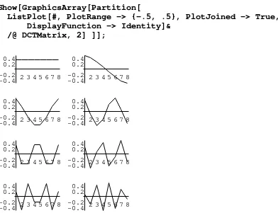
Each element of the transformed list S(u) is the inner (dot) product of the input list s(x) and a
basis vector. The constant factors are chosen so that the basis vectors are orthogonal and
normalized. The eight basis vectors for n = 8 are shown in Figure 1. The DCT can be written as the product of a vector (the input list) and the n x n orthogonal matrix whose rows are the basis vectors. This matrix, for n = 8, can be computed as follows:
DCTMatrix =
Table[ If[ k==0, Sqrt[1/8],
Sqrt[2/8] Cos[Pi (2j + 1) k/16] ], {k, 0, 7}, {j, 0, 7}] // N;
We can check that the matrix is orthogonal:
DCTMatrix . Transpose[DCTMatrix] // Chop // MatrixForm
1. 0 0 0 0 0 0 0
0 1. 0 0 0 0 0 0
0 0 1. 0 0 0 0 0
0 0 0 1. 0 0 0 0
0 0 0 0 1. 0 0 0
0 0 0 0 0 1. 0 0
0 0 0 0 0 0 1. 0
0 0 0 0 0 0 0 1.
Show[GraphicsArray[Partition[
ListPlot[#, PlotRange -> {-.5, .5}, PlotJoined -> True, DisplayFunction -> Identity]&
Figure 1. The eight basis vectors for the discrete cosine transform of length eight.
The list s(x) can be recovered from its transform S(u) by applying the inverse cosine transform (IDCT):
This equation expresses s as a linear combination of the basis vectors. The coefficients are the elements of the transform S, which may be regarded as reflecting the amount of each frequency present in the input s.
We generate a list of random numbers to serve as a test input:
input1 = Table[Random[Real, {-1, 1}], {8}]
{0.203056, 0.980407, 0.35312, -0.106651, 0.0399382, 0.871475,
-0.648355, 0.501067}
output1 = DCTMatrix . input1
{0.775716, 0.3727, 0.185299, 0.0121461, -0.325, -0.993021, 0.559794,
-0.625127}
As noted above, the DCT is closely related to the discrete Fourier transform (DFT). In fact, it is possible to compute the DCT via the DFT (see [Jain 1989, p. 152]): First create a new list by extracting the even elements, followed by the reversed odd elements. Then multiply the DFT of this re-ordered list by so-called "twiddle factors" and take the real part. We can carry out this process for n = 8 using Mathematica's DFT function.
DCTTwiddleFactors = N @ Join[{1},
Table[Sqrt[2] Exp[-I Pi k /16], {k, 7}]]
DCT[list_] := Re[ DCTTwiddleFactors *
InverseFourier[N[list[[{1, 3, 5, 7, 8, 6, 4, 2}]]]]]
Note that we use the function InverseFourier to implement what is usually in engineering called the forward DFT. Likewise, we use Fourier to implement what is usually called the inverse DFT. The function N is used to convert integers to reals because (in Version 2.2)
Fourier and InverseFourier are not evaluated numerically when their arguments are all integers. The special case of a list of zeros needs to be handled separately by overloading the functions, since N of the integer 0 is an integer and not a real. [See In[] and Out[], page ?? --ed.]
Unprotect[Fourier, InverseFourier]; Fourier[x:{0 ..}]:= x;
InverseFourier[x:{0 ..}]:= x; Protect[Fourier, InverseFourier];
We apply DCT to our test input and compare it to the earlier result computed by matrix
multiplication. To compare the results, we subtract them and apply the Chop function to suppress values very close to zero:
DCT[input1]
{0.775716, 0.3727, 0.185299, 0.0121461, -0.325, -0.993021, 0.559794,
-0.625127}
% - output1 // Chop
The inverse DCT can be computed by multiplication with the inverse of the DCT matrix. We illustrate this with our previous example:
Inverse[DCTMatrix] . output1
{0.203056, 0.980407, 0.35312, -0.106651, 0.0399382, 0.871475,
-0.648355, 0.501067}
% - input1 // Chop
{0, 0, 0, 0, 0, 0, 0, 0}
As you might expect, the IDCT can also be computed via the inverse DFT. The "twiddle factors" are the complex conjugates of the DCT factors and the reordering is applied at the end rather than the beginning:
IDCT[DCT[input1]] - input1 // Chop
{0, 0, 0, 0, 0, 0, 0, 0}
The Two-Dimensional DCT
The one-dimensional DCT is useful in processing one-dimensional signals such as speech waveforms. For analysis of two-dimensional (2D) signals such as images, we need a 2D version of the DCT. For an n x m matrix s, the 2D DCT is computed in a simple way: The 1D DCT is
As in the one-dimensional case, each element S(u, v) of the transform is the inner product of the input and a basis function, but in this case, the basis functions are n x m matrices. Each
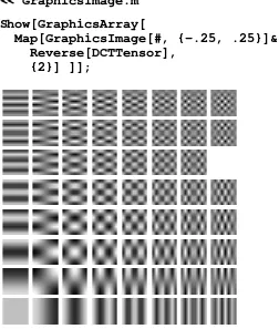
two-dimensional basis matrix is the outer product of two of the one-dimensional basis vectors. For n = m = 8, the following expression creates an 8 x 8 array of the 8 x 8 basis matrices, a tensor with dimensions {8, 8, 8, 8}:
DCTTensor = Array[
Outer[Times, DCTMatrix[[#1]], DCTMatrix[[#2]]]&, {8, 8}];
Each basis matrix can be thought of as an image. The 64 basis images in the array are shown in Figure 2.
The package GraphicsImage.m, included in the electronic supplement, contains the functions
GraphicsImage and ShowImage to create and display a graphics object from a given matrix.
GraphicsImage uses the built-in function Raster to translate a matrix into an array of gray cells. The matrix elements are scaled so that the image spans the full range of graylevels. An optional second argument specifies a range of values to occupy the full grayscale; values outside the range are clipped. The function ShowImage displays the graphics object using Show.
<< GraphicsImage.m
Show[GraphicsArray[
Map[GraphicsImage[#, {-.25, .25}]&, Reverse[DCTTensor],
{2}] ]];
ShowImage[ input2 =
{{0, 1, 0, 0, 0, 1, 0, 0}, {0, 1, 0, 0, 0, 1, 0, 0}, {0, 1, 1, 1, 1, 1, 0, 0}, {0, 1, 0, 0, 0, 1, 0, 0}, {0, 0, 1, 0, 1, 0, 0, 0}, {0, 0, 1, 0, 1, 0, 0, 0}, {0, 0, 1, 0, 1, 0, 0, 0}, {0, 0, 0, 1, 0, 0, 0, 0}}]
-Graphics-As in the 1D case, it is possible to express the 2D DCT as an array of inner products (a tensor contraction):
output2 = Array[
(Plus @@ Flatten[DCTTensor[[#1, #2]] input2])&, {8, 8}];
ShowImage[output2]
-Graphics-The pixels in this DCT image describe the proportion of each two-dimensional basis function present in the input image. The pixels are arranged as above, with horizontal and vertical
frequency increasing from left to right and bottom to top, respectively. The brightest pixel in the lower left corner is known as the DC term, with frequency {0, 0}. It is the average of the pixels in the input, and is typically the largest coefficient in the DCT of "natural" images.
An inverse 2D IDCT can also be computed in terms of DCTTensor; we leave this as an exercise for the reader.
DCT[array_?MatrixQ] :=
Transpose[DCT /@ Transpose[DCT /@ array] ]
This function assumes that its input is an 8 x 8 matrix. It takes the 1D DCT of each row, transposes the result, takes the DCT of each new row, and transposes again. This function is more efficient than computing the tensor contraction shown above, since it exploits the built-in function InverseFourier.
We compare the result of this function to that obtained using contraction of tensors :
DCT[input2] - output2 // Chop // Abs // Max
0
The definition of the inverse 2D DCT is straightforward:
IDCT[array_?MatrixQ] :=
Transpose[IDCT /@ Transpose[IDCT /@ array] ]
As an example, we invert the transform of the letter A:
ShowImage[Chop[IDCT[output2]]];
As noted earlier, the components of the DCT output indicate the magnitude of image components at various 2D spatial frequencies. To illustrate, we can set the last row and column of the DCT of the letter A equal to zero:
output2[[8]] = Table[0, {8}]; Do[output2[[i, 8]] = 0, {i, 8}];
ShowImage[Chop[IDCT[output2]]];
The result is a blurred letter A: the highest horizontal and vertical frequencies have been removed. This is easiest to see when the image is reduced in size so that individual pixels are not as visible.
2D Blocked DCT
To this point, we have defined functions to compute the DCT of a list of length n = 8 and the 2D DCT of an 8 x 8 array. We have restricted our attention to this case partly for simplicity of
exposition, and partly because when it is used for image compression, the DCT is typically restricted to this size. Rather than taking the transformation of the image as a whole, the DCT is applied separately to 8 x 8 blocks of the image. We call this a blocked DCT.
To compute a blocked DCT, we do not actually have to divide the image into blocks. Since the 2D DCT is separable, we can partition each row into lists of length 8, apply the DCT to them, rejoin the resulting lists, and then transpose the whole image and repeat the process:
DCT[list_?(Length[#]>8&)] :=
Join @@ (DCT /@ Partition[list, 8])
It may be worth tracing the progress of this deceptively simple piece of code as it works upon a 16 x 16 image. First, we observe the order in which Mathematica stores the three rules we have given for DCT:
?DCT
Global`DCT
DCT[(array_)?MatrixQ] := Transpose[DCT /@ Transpose[DCT /@ array]]
DCT[(list_)?(Length[#1] > 8 & )] := Apply[Join, DCT /@ Partition[list, 8]]
DCT[list_] := Re[DCTTwiddleFactors*
InverseFourier[N[list[[{1, 3, 5, 7, 8, 6, 4, 2}]]]]]
When DCT is applied to a row of length 16, the second rule comes into play. The row is partitioned into two lists of length 8, and DCT is applied to each. These applications invoke the last rule, which simply computes the 1D DCT of the lists of length 8. The two sub-rows are then rejoined by the second rule. After each row has been transformed in this way, the entire matrix is transposed by the first rule. The process of partitioning, transforming, and rejoining each row is then repeated, and the resulting matrix is transposed again.
For a test image, we provide a small 64 x 64 picture of a space shuttle launch. We use the utility function ReadImageRaw, defined in the package GraphicsImage.m to read a matrix of graylevels from a file:
shuttle = ReadImageRaw["shuttle", {64, 64}];
ShowImage[shuttle]
-Graphics-Applying the DCT to this image gives an image consisting of 8 x 8 blocks, each block a DCT of 8 x 8 pixels:
ShowImage[DCT[shuttle], {-300, 300}]
The inverse DCT of a list of length greater than 8 is defined in the same way as the forward transform:
IDCT[list_?(Length[#]>8&)] :=
Join @@ (IDCT /@ Partition[list, 8])
Here is a simple test:
shuttle - IDCT[DCT[shuttle]] // Chop // Abs // Max
0
Quantization
DCT-based image compression relies on two techniques to reduce the data required to represent the image. The first is quantization of the image's DCT coefficients; the second is entropy coding
of the quantized coefficients. Quantization is the process of reducing the number of possible values of a quantity, thereby reducing the number of bits needed to represent it. Entropy coding is a technique for representing the quantized data as compactly as possible. We will develop
functions to quantize images and to calculate the level of compression provided by different degrees of quantization. We will not implement the entropy coding required to create a compressed image file.
A simple example of quantization is the rounding of reals into integers. To represent a real number between 0 and 7 to some specified precision takes many bits. Rounding the number to the nearest integer gives a quantity that can be represented by just three bits.
x = Random[Real, {0, 7}]
2.78452
Round[x]
3
In this process, we reduce the number of possible values of the quantity (and thus the number of bits needed to represent it) at the cost of losing information. A "finer" quantization, that allows more values and loses less information, can be obtained by dividing the number by a weight factor before rounding:
w = 1/4;
Round[x/w]
11
Taking a larger value for the weight gives a "coarser" quantization.
w * % // N
2.75
The quantization error is the change in a quantity after quantization and dequantization. The largest possible quantization error is half the value of the quantization weight.
In the JPEG image compression standard, each DCT coefficient is quantized using a weight that depends on the frequencies for that coefficient. The coefficients in each 8 x 8 block are divided by a corresponding entry of an 8 x 8 quantization matrix, and the result is rounded to the nearest integer.
In general, higher spatial frequencies are less visible to the human eye than low frequencies. Therefore, the quantization factors are usually chosen to be larger for the higher frequencies. The following quantization matrix is widely used for monochrome images and for the luminance component of a color image. It is given in the JPEG standards documents, yet is not part of the standard, so we call it the "de facto" matrix:
qLum =
{{16, 11, 10, 16, 24, 40, 51, 61}, {12, 12, 14, 19, 26, 58, 60, 55}, {14, 13, 16, 24, 40, 57, 69, 56}, {14, 17, 22, 29, 51, 87, 80, 62}, {18, 22, 37, 56, 68,109,103, 77}, {24, 35, 55, 64, 81,104,113, 92}, {49, 64, 78, 87,103,121,120,101}, {72, 92, 95, 98,112,100,103, 99}};
Displaying the matrix as a grayscale image shows the dependence of the quantization factors on the frequencies:
ShowImage[qLum];
To implement the quantization process, we must partition the transformed image into 8 x 8 blocks:
BlockImage[image_, blocksize_:{8, 8}] := Partition[image, blocksize] /;
And @@ IntegerQ /@ (Dimensions[image]/blocksize)
UnBlockImage[blocks_] := Partition[
Flatten[Transpose[blocks, {1, 3, 2}]], {Times @@ Dimensions[blocks][[{2, 4}]]}]
For example:
Table[i + 8(j-1), {j, 4}, {i, 6}] // MatrixForm
1 2 3 4 5 6
9 10 11 12 13 14
17 18 19 20 21 22
25 26 27 28 29 30
BlockImage[%, {2, 3}] // MatrixForm
1 2 3 4 5 6 9 10 11 12 13 14
17 18 19 20 21 22 25 26 27 28 29 30
UnBlockImage[%] // MatrixForm
1 2 3 4 5 6
9 10 11 12 13 14
17 18 19 20 21 22
25 26 27 28 29 30
Our quantization function blocks the image, divides each block (element-by-element) by the quantization matrix, reassembles the blocks, and then rounds the entries to the nearest integer:
DCTQ[image_, qMatrix_] := Map[(#/qMatrix)&,
BlockImage[image, Dimensions[qMatrix]], {2}] // UnBlockImage // Round
The dequantization function blocks the matrix, multiplies each block by the quantization factors, and reassembles the matrix:
IDCTQ[image_, qMatrix_] := Map[(# qMatrix)&,
BlockImage[image, Dimensions[qMatrix]], {2}] // UnBlockImage
To show the effect of quantization, we will transform, quantize, and reconstruct our image of the shuttle using the quantization matrix introduced above:
qshuttle = shuttle //
For comparison, we show the original image together with the quantized version:
Show[GraphicsArray[
GraphicsImage[#, {0, 255}]& /@ {shuttle, qshuttle}]];
Note that some artifacts are visible, particularly around high-contrast edges. In the next section, we will compare the visual effects and the amount of compression obtained from different degrees of quantization.
Entropy
To measure how much compression is obtained from a quantization matrix, we use a famous theorem of Claude Shannon [Shannon and Weaver 1949]. The theorem states that for a sequence of symbols with no correlations beyond first order, no code can be devised to represent the sequence that uses fewer bits per symbol than the first-order entropy, which is given by
h= − pilog2( )pi
i
ε
where pi is the relative frequency of the ith symbol.
To compute the first-order entropy of a list of numbers, we use the function Frequencies, from the standard package Statistics`DataManipulation`. This function computes the relative frequencies of elements in a list:
(shac poisson) In[1 ]:= (7 /1 2 /9 4 at 8 :5 8 :2 6 A M )
Frequencies[list_List] :=
Map[{Count[list, #], #}&, Union[list]]
Characters["mississippi"]
{m, i, s, s, i, s, s, i, p, p, i}
Frequencies[%]
{{4, i}, {1, m}, {2, p}, {4, s}}
Entropy[list_] :=
- Plus @@ N[# Log[2, #]]& @
(First[Transpose[Frequencies[list]]]/Length[list])
For example, the entropy of a list of four distinct symbols is 2, so 2 bits are required to code each symbol:
Entropy[{"a", "b", "c", "d"}]
2.
Similarly, 1.82307 bits are required for this longer list with four symbols:
Entropy[Characters["mississippi"]]
1.82307
A list with more symbols and fewer repetitions requires more bits per symbol:
Entropy[Characters["california"]]
2.92193
The appearance of fractional bits may be puzzling to some readers, since we think of a bit as a minimal, indivisible unit of information. Fractional bits are a natural outcome of the use of what are called "variable word-length" codes. Consider an image containing 63 pixels with a greylevel of 255, and one pixel with a graylevel of 0. If we employed a code which used a symbol of length 1 bit to represent 255, and a symbol of length 2 bits to represent 0, then we would need 65 bits to represent the image, or in terms of the average bit-rate, 65/64 = 1.0156 bits/pixel. The entropy as calculated above is a lower bound on this average bit-rate.
The compression ratio is another frequently used measure of how effectively an image has been compressed. It is simply the ratio of the size of the image file before and after compression. It is equal to the ratio of bit-rates, in bits/pixel, before and after compression. Since the initial bit-rate is usually 8 bits/pixel, and the entropy is our estimate of the compressed bit-rate, the compression ratio is estimated by 8/entropy.
We will use the following function to examine the effects of quantization:
f[image_, qMatrix_] :=
{Entropy[Flatten[#]], IDCT[IDCTQ[#, qMatrix]]}& @ DCTQ[DCT[image], qMatrix]
This function transforms and quantizes an image, computes the entropy, and dequantizes and reconstructs the image. It returns the entropy and the resulting image. A simple way to experiment with different degrees of quantization is to divide the "de facto" matrix qLum by a scalar and look at the results for various values of this parameter:
test = f[shuttle, qLum/#]& /@ {1/4, 1/2, 1, 4};
Show[GraphicsArray[ Partition[
Apply[
ShowImage[#2, {0, 255}, PlotLabel -> #1, DisplayFunction -> Identity]&,
test, 1], 2] ] ]
1.7534 3.10061
0.838331 1.25015
-GraphicsArray-Timing
Most of the computation time required to transform, quantize, dequantize, and reconstruct an image is spent on forward and inverse DCT calculations. Because these transforms are applied to blocks, the time required is proportional to the size of the image. On a SUN Sparcstation 2, the timings increase (at a rate of 0.005 second/pixel) from about 20 seconds for a 642 pixel image to about 320 seconds for 2562 pixels.
References
Ahmed, N., T. Natarajan, and K. R. Rao. 1974. On image processing and a discrete cosine transform. IEEE Transactions on Computers C-23(1): 90-93.
Chen, W. H., and W. K. Pratt. 1984. Scene adaptive coder. IEEE Transactions on Communications COM-32: 225-232.
Jain, A. K. 1989. Fundamentals of digital image processing . Prentice Hall: Englewood Cliffs, NJ.
Puri, A. 1992. Video coding using the MPEG-1 compression standard. Society for Information Display Digest of Technical Papers 23: 123-126.
Shannon, C. E., and W. Weaver. 1949. The mathematical theory of communication . Urbana: University of Illinois Press.
Wallace, G. 1991. The JPEG still picture compression standard. Communications of the ACM 34(4): 30-44.
Watson, A. B. 1993. DCT quantization matrices visually optimized for individual images. Proceedings of the SPIE 1913: 202-216 (Human Vision, Visual Processing, and Digital Display IV. Rogowitz ed. SPIE. Bellingham, WA).
Biography
Andrew B. Watson is the Senior Scientist for Vision Research at NASA Ames Research Center in Mountain View, California, where he works on models of visual perception and their
application to the coding, understanding, and display of visual information. He is the author of over 60 articles on human vision, image processing, and robotic vision.
Electronic Supplement
The electronic supplement contains the packages DCT.m and GraphicsImage.m, and the image file shuttle.
Andrew B. Watson
NASA Ames Research Center